Design of a numerical solar dynamo model.

-1-DESIGN OF A NUMERICAL SOLAR DY.NAMO MODEL

by

CHARLES TONY GORDON B.S., University of Chicago

(194)

SUBMITTED IN PARTIAL FULFILLMENT OF THE REQUIREMENTS FOR THE DEGREE OF

DOCTOR OF PHILOSOPHY at the

MASSACHUSETTS INSTITUTF OF TECHNOLOGY November, 1970L t .. Signature of Author ... Certified by ... ... . .. Accepted by...,...,,.a o o0 o9 o 0 0 a oo 00000 .t ... .... ... .... Department of Meteorology o a a 0 0 a 0 a 0 -o 9 ,- 9 0 O . . 0 o o o o o .0 O o a 0 O 0 o o o o O Thesis Supervisor

Chairman, Departmental Committee on Graduate Students

MITLibraries

Document Services

Room 14-0551 77 Massachusetts Avenue Cambridge, MA 02139 Ph: 617.253.5668 Fax: 617.253.1690 Email: docs@mit.edu http://libraries.mit.edu/docs

DISCLAIMER OF QUALITY

Due to the condition of the original material, there are unavoidable

flaws in this reproduction. We have made every effort possible to

provide you with the best copy available. If you are dissatisfied with

this product and find it unusable, please contact Document Services as

soon as possible.

Thank you.

Due to the poor quality of the original document, there is

some spotting or background shading in this document.

-2-DESIGN OF A NUMERICAL SOLAR DYNAMO MODEL by

Charles Tony Gordon

Submitted to the Department of Meteorology on November 30, 1970 partial fulfillment of the requirements for the

degree of Doctor of Philosphy

ABSTRACT

Observations and theories of the solar differential rotation and of large scale solar magnetic fields are reviewed. The fluid dynamo ap-proach is emphasized for the maintenance of magnetic fields. A numerical, hydromagnetic dynamo model is then formulated. It has two layers and is baroclinically driven. Its principal new features for a model of this type

are thin shell spherical geometry, a Robert (equivalent to a spherical har-monic) spectral representation on spherical surfaces, and "primitive" hydro-magnetic equations. Magnetic fields are allowed to penetrate across the upper boundary.

A time averaged, zonally averaged angular momentum balance is achieved locally, only if the angular momentum equations (A.M.E.) are

"correctly truncated". This is attributed to both the spectral represen-tation and low model resolution. In contrast, the surface integral of the A.M.E. and the energy integrals derived for the model are preserved by the orthogonal truncation process.

Numerical integration of the low resolution model yields computa-tionally stable solutions. The model is applied to the sun. For two of five thermal forcing profiles examined in the nonmagnetic case, a horizon-tal differential rotation of the required strength develops and is main-tained by horizontal eddy transports. The streamline patterns are usually tilted upstream away from the relative velocity jet. Fultz's dishpan exper-ments and Ward's sunspot statistics lend credence to the above results.

For four of the thermal forcing profiles, analogous magnetic runs are made to study, qualitatively, magnetic feedback upon the flow. In this context, two magnetic production runs are discussed in detail for the case of approximate equipakrtion of kinetic and magnetic energy. In neither run do the magnetic fields reverse the sign of the horizontal eddy transport of angular momentum. Nevertheless, the strong magnetic feedback has several consequences including weaker eddy transports and a somewhat stronger meri-dional circulation. In addition, the horizontal shear of the vertically averaged angular velocity profile is almost totally destroyed. The horizon-tal axisymmetric Reynolds and Maxwell stresses play very important roles in the vertically averaged angular momentum balance.

At the upper level, the horizontal differential rotation has the correct sign in both magnetic production runs. Thus, in P.R. 1, i.e., the production run with warm equator-cold pole thermal forcing, the horizontal shear has reversed sign there, but is too weak by a factor of --6, when strong magnetic fields have developed. The horizontal shear decreases, yet remains of the correct order of magnitude in magnetic P.R. 2, i.e., the

production run with warm pole-cold equator forcing. A crude determination of the RosEby-Hadley regime boundary is mnde for P.R. 2.

Regarding magnetic induction, magnetic fields are generated and then sustained by dynamo action, provided the magnetic Reynolds number ex-ceeds a critical value. This value apparently varies with the type of

thermal forcing profile and with model resolution. Illustrations are given of magnetic field patterns, mainly for both production runs. In a very

crude sense, the vertical magnetic eddies may be identified with solar mag-netic active regions. But except during the first 12 years of P.R. 1, they do not generally tilt persistently in the proper sense.

In the attempted simulation of the solar magnetic cycle, the re-versals of axisymmetric poloidal (nd toroidal) magnetic fields is an en-couraging result. For the run having the less realistic angular velocity profile at the upper level, i.e., P.R. 1, the mean reversal time of 11 to 12 years is in rather good agreement with the presumed solar value. But the reversals are irregular. For P.R. 2, the mean reversal time of 1 to 2 years is about an order of magnitude too small.

The energetics of both magnetic runs and their implications for the maintenance of the dynamo are discussed. In its grossest aspects, the reversal process appears to resemble Gilman's, except that poloidal fields are stretched into toroidal fields by the vertical shear of the differential rotation. Some other phenomena related.to the magnetic reversals are

briefly described for our model. It is found that the generalized Sp6rer's law for the equatorward migration of the zone of maximum solar magnetic activity is not obeyed.

A critique of our results and suggestions for future numerical research are given.

Thesis Supervisor: Victor P. Starr Title: Professor of Meteorology

-4-.

TABLE OF CONTENTS

CHAPTER I. THE EQUATORIAL JET AND MAGNETIC FIELDS IN

THE SOLAR ATMOSPHERE 11

1.1. Introduction Ill

1.2. Solar Observations 11

1.2.1. A rough view of the sun 11

1.2.2. Observational length and time scales 12

1.2.3. Observational evidence, for the existence and

maintenance of the equatorial jet 14

1.2.4. Observations of large scale magnetic fields 21 1.3. Theories of the Solar Differential Rotation 28

1.3.1. Axisymmetric theories 29

1.3.2. Asymmetric theories 36

1.4. Theories of Magnetic Fields , 47

1.4.1. Fluid dynamos 48

1.4.2. Maintenance of the observed solar magnetic field 59

1.5. Characteristics of our Dynamo Model 70

1.6. Summary of the Other Chapters 74

CHAPTER II. FORMULATION OF THE SPHERICAL HYDROMAGNETIC DYNAMO

MODEL WITH BAROCLINIC HEATING 77

2.1. Introduction 77

2.2. Basic Assumptions 77

2.3. The Equations 82

2.4. The MHD Approximation 88

2.5. Further Refinements and Simplifications 81

2.5.1. The "primitive" equations 91

2.5.2. The thermodynamics 101

TABLE OF CONTENTS (cuntinued)

CHAPTER III. THE NUMERICAL TWO LAYER SPECTRAL MODEL 110

3.1. Introductory Remarks 110

3.2. Representation of Vertical Variation by Two Layers 110 3.3. Interior Equations for the Two Layer Model 113

3.4. The Spectral Representation 122

3.4.1. The correspondence between spherical harmonics

and Robert functions 123

3.4.2. Details of the Robert spectral method 126

3.5. The Time Differencing Scheme 137

3.6. Sequence of Equations to be Solved 138

CHAPTER IV. FORMULATION OF A "CORRECTLY TRUNCATED" ANGULAR

MOMENTUM BALANCE 143

4.1. Introduction 143

4.2. The Angular Momentum Equations 143

4.3. Inconsistencies in the Untruncated Angular Momentum

Balance 149

4.4. Analysis of the "Correctly Truncated" Angular Momentum

Balance 150

CHAPTER V. FORMULATION OF THE ENERGY BALANCE 164

CHAPTER VI. NUMERICAL RESULTS 181

6.1. Introduction 181

6.2. Simulation of the Terrestrial Atmosphere - Test Run 1 182 6.3. Summary of Runs and Parameters for the Solar Model 185

6.4. The Effects of Thermal Forcing Profile Type and Magnetic

Fields upon the Angular Velocity Profile 188

6.5. General Circulation Statistics for Production Runs 1 and 2 199

6.5.1. Production Run 1 200

TABLE OF CONTENTS (continued)

6.6. The Search for Dynamo Solutions

6.7. Basic Structure of the Magnetic Field Solutions 6.7.1. Solutions for Production Run 1

6.7.2. Solutions for Production Run 2

6.8. Magnetic Field Reversals and Dynamo Maintenance 6.8.1. Observations and Other Theories of Solar

Magnetic Reversals

6.8.2. Simulation of Magnetic Reversals by our Model

6.8.3. The Energetics of the Model and Its Implications

for Dynamo Maintenance

6.8.4. Further Discussion of Dynamo Maintenance 6.8.5. Spirer's Law and Possibly Related Phenomena CHAPTER VII. CONCLUSIONS AND SUGGESTIONS FOR FUTURE RESEARCH

APPENDIX A. APPENDIX B. APPENDIX C.

POLOIDAL AND TOROIDAL VECTOR SPHERICAL HARMONICS PROGRAMMING THE NUMERICAL INTEGRATION

ENERGY INTEGRALS FOR A CONTINUOUS, QUASI-BOUSSINESQ MODEL BIBLIOGRAPHY ACKNOWLEDGEMENTS BIOGRAPHICAL NOTE 220 223 224 231 238 238 239 243 252 253 261 269 271 272 277 286 287

-G-Fig. 1.1. Fig. Fig. Fig. Fig. Fig. Fig. Fig. Fig. 3.1. 4.1. 4.2. 5.1a. 5.lb. 5.2a. 5.2b. 6.1. Fig. 6.2. Fig. 6.3a. Fig. 6.3b. Fig. Fig. 6.4. 6.5. Fig. 6.6. Fig. 6.7. Fig. 6.8. Fig. 6.9.

Synoptic chart of line of sight solar magnetic fields (from Bumba and Howard (1965b) ).

Schematic diagram of two layer model.

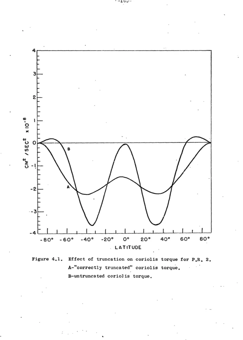
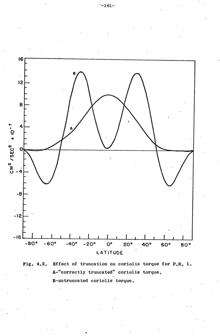
Effect of truncation on coriolis torque for P.R. 2. Effect of truncation on coriolis torque for P.R. 1. Energy diagram for the generalized magnetic case, Energy diagram for the nonmagnetic case.

Energy diagram for toroidal motion anti-dynamo. Energy diagram for axisymmetric anti-dynamo. General circulation statistics for terrestrial atmosphere test run.

Four types of thermal forcing profiles. These profiles have been quasi-normalized,

Absolute angular velocity /L profiles for test run .7

Perturbation potential temperature and thermal forcing profiles for test run 7.

Some general circulation statistics for P.R. 1. Comparison of absolute angular velocity profiles

of magnetic P.R. 1 with observations.

Vertically averaged angular momentum balance of magnetic P.R. 1.

Vertically averaged horizontal Reynolds stresses and Maxwell stresses of magnetic P.R. 1,

Some general circulation statistics for P.R. 2,

25 113 160 161 179 179 179 179 186 190 196 196 203 205 206 207 212 Comparison of absolute angular velocity profiles

of magnetic P.R. 2 with observations." '. 214

LIST OF FIGURES (continued) Fig. 6.10. Fig. 6.11. Fig. 6.12. Fig. 6.13. Fig. Fig. Fig. Fig. Fig. Sig. Fig. Fig. 6.14. 6.15. 6.16. 6.17. 6.18. 6.19. 6.20. 6.21. Fig. 6.22. Fig. 6.23. Fig. Fig. Fig. Fig. 6.24. 6.25. 6.26. 6.27.

Vertically averaged angular momentum balance of magnetic P.R. 2.

Vertically averaged horizontal Reynolds stresses and Maxwell stresses of magnetic p.R. 2.

Crude determination of the Rossby regime-Hadley regime boundary for nonmagnetic P.R. 2.

Time evolution of horizontal magnetic field 3 for P,;R. 1, at intervals of 10 solar rotations,

1 for P.R. 1,

I for P.R. I,

Stream function r, for P.R. 1 at t=0.69 yrs. i. before significant dynamo action occurs.

Sample solutions for P.R. 1 at t=8.20 yrs.

Time evolution of horizontal magnetic field

,.

for P.R. 2 at intervals of 10 solar rotations.

Sample solutions for P.R. 2 at t=24.60 yrs.

Vertical magnetic fields for P.R. 2 at t=28.08 yrs. Stream function VPIr for test run 7 at t=l.ll yrs.,i -before significant dynamo action occurs.

Horizontal magnetic field B for test run 7 at

H

3.89 yrs.

Magnetic fields for test run 12 (Rm = 500) at t=21.75 yrs.

Time reversal of polar magnetic fields for P.R. 1. Time reversal of polar magnetic fields for P.R. 2. Energy diagram for magnetic P.R. 1.

Energy diagram for magnetic P.R. 2.

215 216 219 227 229 229 229 230 233 235 236 237 237 237 241 242 244 245 0 . .0

LIST OF FIGURES (continued) Fig. 6.28. Fig. 6.29. Fig. 6.30a. Fig. 6.30b. Fig. 6.31a. Fig. 6.31b.

Meridional-time cross section of axisymmetric toroidal and vertical magnetic fields for P.R. 1. Meridional-time cross section of axisymmetric

toroidal and vertical magnetic fields for P.R. 2, Superposition of regions of strong vertical eddy motions upon the meridional-time cross section of

<8 > of Fig. 6.28a for P.R. 1.

Superposition of regions of strong vertical eddy

motions upon the meridional-time cross section of

<B8"> of Fig. 6.29a for P.R. 2,

Meridional-time cross section of the vertically averaged zonal wind <Et2> in P.R. 2.

Time evolution of the square of the Alfven number

256 257 258 258 259 259

-I)-LTIT OF TABLES Table 1.1. Table 4.1. Table 4.2. Table 6.1. Table 6.2. Table 6.3. Table 6.4.

Latitude Distribution of Sunspots as a Function of Time (from Ward (1964) ).

Catalogue of Terms in the Angular Momentum Balance Equations.

Useful Properties of Some Low Order Legendre Polynomials.

Specified Parameters for the Earth and Sun, Catalogue of Test Runs and Production Runs for Solar Model.

I

Qualitative Effects of the Y, Profile on Velocity Shear for Nonmagnetic and Magnetic Cases.

Dynamo Behavior for Different Runs.

20 146 154 183 189 192 222

CHAPTER I. THE EQUATORIAL JET AND MAGNETIC FIELDS IN THE SOLAR ATMOSPHERE

1.1, Introduction.

The existence and maintenance of the solar equatorial jet and the large scale solar magnetic fields will be a central theme of

this study. In Chapter I, the basic observational evidence relating to the equatorial jet and to large scale magnetic fields will first be re-viewed. The discussion then turns to various possible physical mecha-nisms for maintaining the jet. As for the maintenance of the magnetic fields, the self-sustaining fluid dynamo approach is emphasized. In

this connection, a survey of the literature on dynamo theory has reveal-ed certain basic properties of fluid dynamos.

In the concluding part of Chapter I, a self-consistent model which contains various essential ingredients already enumerated, is pro-posed. In principle, the model is capable of dynamo generation and

main-tenance. The chief departures from a recent numerical dynamo study by Gilman (1968) include the adoption of the "primitive" hydromagnetic equations and thin shell spherical geometry. When these modifications are coupled with suitably adjusted baroclinic thermal forcing, an equa-torial acceleration is possible.

1.2. Solar Observations,

1.2.1. A rough view of the sun.

The basic solar data consists of continuum emission, absorp-tion lines, and emission lines. This'radiaabsorp-tion reflects the local values of wind, temperature, density, magnetic field strength, composition, and

-12-state of ionization averaged long the line of sight. The most serious observational limitation is due to the opacity of the solar disk. Even in white light, only its uppermost few hundred kilometers are visible.

A rough picture of the solar interior has emerged, however, from stellar model calculations of Schwarzschild (1958) and others. Thus the sun probably has a convective envelope, and a radiative core in which a thermonuclear core is imbedded. Denoting the solar radius by Re , the radiative core-convection zone interface lies between 0.8 R and-0.9 R. , while the upper boundary of the convection zone lies just beneath the

visible surface. The observed photospheric "granulation" would then represent small scale convection which has penetrated this upper

boundary. Speculation on the more detailed temperature structure within the convection zone is deferred until later.

The 5 x 103 oK photophere is separated from the overlying

1.5 x 106 oK corona by a sharp transition region known as the chromosphere.

The continuum emission originates mainly from the photosphere and lower chromosphere. Absorption lines are also formed there, while emission lines are formed predominantly in the corona and-upper chromosphere.

1.2.2. Observational length and time scales.

Solar observations reveal hydrodynamic and magnetic phenomena over a broad range of time and space scales. Near the short end of the spectrum is the granulation. An individual granule has a characteristic size of 700 km and a lifetime of 8 minutes (Zirin, 1966). These scales

rYe

SMall compared to the sun's radius (Rez 6.95 x 105 km).and observed mean rotation period ( T, 25.4 sideral days). Photospheric cellular hori-zontal motion patterns, dubbed supergranules, have a diameter of about

3 x 104 km and a mean lifetime of 20 hours (Simon and Leighton, 1964).

Supersupergranulation, i.e., convective cells with a characteristic dimension of several hundred thousand kilometers may have been observed

(Bumba, 1967). Horizontal eddy motions of similar size are implied by Ward's (1964) and later studies.

A very large sunspot group may encompass 0.3% of the solar disk area (Zirin,19E6), which is roughly supergranular size. But spots are imbedded in active regions having lateral dimensions of up to 2 x 105 km (Bumba and Howard, 1961b). Comparably large scale magnetic fields having intenSities of several gauss are another manifestation of active regions (Bumba and Howard, 1965b). These magnetic fields as well as active regions and large sunspots may persist for several rotations. A polarity reversal of the leader and follower spot magnetic fields is a feature of the double sunspot cycle2_.

The large scale, axisymmetric poloidal field, i.e., the axisymmetric component in meridional planes, also seems to undergo such a reversal. The average length of the double sunspot cycle is 22 years. Finally, an equatorial jet is a quasi-per-. manent feature, and not just a statistical remnant of the solar general circulation. Of chief interest to us will be phenomena having large length and time scales.

2

The various characteristics of the sunspot cycle are conveniently summarized by Babcock (1961).

-14-1.2.3. Observational evidence for the existence and maintenance of the equatorial jet.

"Observations" of the Differential Rotation.

Three methods of observing motions in the solar atmosphere are (1) tracing sunspot displacements, (2) tracing other definable fea-tures such as filaments and (3) measuring Doppler line shifts. Sunspot data is the most comprehensive. Since 1874, sunspot group positions

(in tenths of degrees of latitude and longitude) have been extracted and tabulated once each day, from photographs taken principally at the

Greenwich or Cape Observatories.

Newton and Nunn (1951) measured the time interval between successive central meridian passages of longlived, generally large

sun-3

spots from recurrent sunspot data for the period 1878-1944. By a least squares technique, they obtained the angular velocity profile

Ai

- 8 o

237

7

, x/nQ longitude per day (1.1)

C- being the latitude.

'As an alternative to Newton and Nunn's procedure, Ward (1964)

computed displacements of shortlived and longlived spots. His angular velocity profile agreed with equation (1.1) to within a few percent. Ward (1966) noted that the daily motions of small spots predict an angu-lar rotation rate slightly angu-larger than equation (1.1) near the equator

and 2% larger at 300. Moreover, elongated spots seemed to move up to 2%

Recurrent sunspots reappear at least once on the east limb (look-ing toward the sun) of the solar disk.

faster than circularly shaped spots.

An auto-correlation analysis of the local magnetic polarity

in active regions has recently been performed by Wilcox and Howard (1970) based upon roughly seven years of data, A mean differential rotation qualitatively similar to equation (1.17 may be inferred from the sharp peaks at 26 to 29 synodic days in the auto-correlation curves for differ-ent latitudes.

Filaments can be found at more poleward latitudes than sun-spots, tend to be elongated, and are of chromospheric rather than of photospheric origin (Zirin, 1966). The angular velocity profile deter-mined from filament displacements by ,. and L. d'Azambuja (1948) agrees qualitatively with (1.1) but the angular velocities are slightly larger.

Since 1966, Dr. Howard has obtained Doppler shift measure-ments at 11,000 points over nearly the whole disk on an almost daily

basis. Howard and uarvey (1970) comment in fact that "the analysis of the 1st day's observation combined more individual measures of rotation

Doppler line shifts than were collected in all such previous endeavors", Obtaining a least squares fit to their data, they found

13.76 - 1.74sin 2 - 2.19 sin 4e per day. (1.2)

Note that the equatorial value is some 4% less than in (1.1). It also happens to be in fairly good agreement with other recent spectroscopic

determinations, Secondly, the shear is less pronounced in (1.2) than in (1.1) at sunspot latitudes. The probable errors of the coefficients in (1.2) were estimated to be of order 0,1%, 10%, and 10%, respectively. Rased upon a small sample of Doppler measurements, Plaskett(1962) found

-16-a m-16-aximum -16-angul-16-ar velocity -16-at CL=22 , although his equatorial value agreed with (1.2).

Unlike sunspot heights, the heights of different spectral line formation can be estimated. Thus, Doppler measurements could be use-.ful to help determine height variations in JLo" In a review article,

Bumba (1967) cites Aslanov's results on the variation of (zonally-aver-aged) solar equatorial zonal-velocity, o . From optical depth .111 to

.010, (a 210 km thick layer) Q, increases montonically with height by

12%, whereas from optical depth .125 to .111, LC. decreases with height. Comparison of the filament and sunspot rotation laws suggests L,, in-creases with height, but the primary effect could be the shape of the filaments rather than their location in the chromosphere.

Mean Meridional Velocities

Ward (1964) attempted to compute the space-time mean merid-ional velocity fv] from daily displacements of sunspots. But the 5% con-fidence limits exceeded the magnitude of the computed v's everywhere except in the 0-5oN latitude belt. Within the sunspot latitude belt, the

largest possible magnitude for [v] consistent with the confidence limits was slightly under 20 m/sec.

Even earlier, Plaskett (1962) attempted to determine fvj from line of sight spectroscopic measurements. Unfortunately, the sign of the meridional velocity depended upon which wavelength standard was adopted. Nevertheless he felt that the'observed' meridional velocity was equator-ward. No similar attempt has been made yet with Howard's 1966-1969 data. In principle, coefficients.of a fv3 profile and their probable errors

could be estimated from his spectroscopic data. Horizontal Eddy Motions and Eddy Momentum Transports

Ward (1964) has computed the space-time covariance u'v'J = £uvi -

Lu

v) and the associated correlation coefficients from the daily sunspot displacements. The zonal velocity u and meridional velocity v are measured in the Greenwich reference frame whose rotation rate is-14.1840 per day. Space-time averaging (denoted by

f 3

) weights each spot group equally and is appropriate considering the nature of the data. The u and v components are significantly correlated so that faster ro-tating spots tend to move towards the equator. If streamlines could be drawn, the trough and ridge lines would probably tilt

northwest-south-east (in the northern hemisphere). The eddy momentum transport is up the angular velocity gradient. Ward (1964) estimated the decay time of the differential rotation at just a few rotations if the eddy momentum transport were cut off and not replaced. Starr and Gilman (1965a) show-ed that Ward's results implishow-ed a systematic conversion by horizontal eddies of eddy kinetic energy into kinetic energy of the mean zonal flow at sunspot latitudes.

Hart (1956) demonstrated that observed fluctuations of the Doppler line of sight velocity VL were above the noise level and coherent

for at least an hour. The fluctuations had a weak spectral peak near

2.6 x 104 km and an RMS value of 0(100 m/sec ). Howard and Harvey .(1970)

thought they detected fluctuations with a comparable length scale and a time scale of several days, in addition to a much longer secular varia-tion of J .

-Is

It may even be possible to construct a zeroth order approxi-mation of the large scale flow pattern from Howard's VL data by

retriev-ing the eddy motions from the residual velocities defined by Howard and Harvey (1970). One would assume (1) the large scale vel'city field is horizontal and nondivergent, i.e., can be specified by a stream function CY, , and (2) the equator is a streamline (at least as an initial guess). Then a linear first order partial differential equation in /

relates / to the observed VL values integrated (numerically) by the L

method of characteristics. A necessary condition for assumption (1) to be valid is that VL be small near the center of the disk. Hopefully, the

streamline patterns would be tilted in a manner consistent with Ward's (1964) results.

Ambiguities in the Observational Data

There are certain ambiguities in the interpretation of the data mentioned thus far. A very crucial assumption is that sunspots are good tracers of the large scale flow. An interesting indirect check was made byMacDonald (1966) who used migratory cyclones and anticyclones as tracers of the angular velocity and eddy motions in the terrestrial atmos-phere. The predicted eddy momentum transport was only 1/3 the observed transport. Nevertheless, the predicted shapes of both the eddy momentum transport and absolute angular velocity profiles agree fairly well with the(vertically averaged) observations, except near the equator where cyclone and anticyclone data was scarce. MacDonald reasoned that if the migratory cyclones and anticyclones were satisfactory tracers, then by analogy, sunspots could be too.

It has already been noted that size and shape and life ex-pectancy of sunspots affect how fast they move. Spots also move faster in the incipient as compared to later stages of development (Ward, 1966). In addition, the equivalent height of the circulation traced out by sun-spots is not clear. Sunsun-spots are thought to be manifestations of hydro-magnetic disturbances in the conoction zone. Ward (1964) speculated that spots of greatest vertical extent (which might include the large re-current spots) move the slowest.

Even assuming that sunspots (groups) are good tracers,

positional errors of sunspots (center of gravity of groups) might serious-ly affect the results. For example, sunspot positions are least accur-ately known near the edges of the disk due to foreshortening. Ward (1964) counteracted this difficulty by discarding sunspot data close to the disk edges. _{Even worse, the birth of a new sunspot and death of an old one} between observations or change in structure of a sunspot group could be misinterpreted as sunspot motion. Suspicions were advanced that Ward's

(1964) eddy correlations might be due largely to systematic errors in the center of gravity position of sunspot groups along the spot group axis, which was preferentially tilted NW-SE (NE-SW) in the northern (southern) hemisphere. But Ward (19C5b)refuted the brunt of this argument by

ob-taining significant correlations from displacements of single spots. Also, the correlations basically held up when sunspot displacements ex-ceeding critical longitude and/or latitude values were screened out (Ward, 1964).

Table 1.1. Latitude distribution of sunspots as a function of time (from Ward (1964)).

Table 2

Number of Observations

(Cutoff: 1.0* Lat., 1.50 Long.)

North South Year > 30 30-25 25-20 20-15 15-10 10-5 5-0 0-5 5-10 10-15 15-20 20-25 25-30

>

30 Total 1935 16 76 115 40 25 0 5 2 4 23 102 93 78 47 626 1936 25 44 129 188 138 18 0 0 33 149 229 160 89 74 1276 1937 58 52 179 225 367 179 9 1 106 226 204 141 F 6 24 1827 1938 3 69 128 142 255 137 50 29 251 220 188 120 6 12 1669 1939 2 59 74 158 178 167 41 41 241 233 238 67 2 9 1510 1940 0 2 20 90 176 168 26 33 239 233 90 22 1 0 1100 1941 0 1 5 46 204 113 68 68 137 78 27 0 0 0 747 1942 0 0 4 21 98 132 12 36 101 105 I 0 0 0 510 1943 0 0 0 9 47 86 38 26 22 12 I 8 2 1 252 1944 4 7 21 9 1 11 9 0 14 0 0 50 17 7 150 1935-44 108 310 675 928 1489 1011 258 236 1148 1279 1080 661 310 174 9667

1935-44 282 620 1336 2008 2768 2159 494 (9667) North and South Total (Cutoff: 1.00, 1.50)

1935-44 335 753 1569 2361 3203 2519 574 (11 314) North and South Total (Cutoff: 2.00, 3.0*)

latitude distribution and total number of sunspots varies dramatically over the sunspot cycle. Thus a formula like (1.1) might reflect a time variation as well as latitudinal variation of the solar rotation. The

reduction of spectroscopic data of Livingston (1969) and of Howard and Harvey (-1970) suggests that whereas a positive solar equatorial jet is prezent on most days, the profilee does vary with time.

It may be noted that the Doppler line shift measurements con-tain various systematic and random errors. The orbital motion and rota-tion of the earth must be- subtracted out as well as the red shift at the limb (- 340 m/sec). Also, the arbitrary zero reference may shift from day to day or even during the 90 minute scan of the disk. A pressure fluctuation of only 0.13 mb will produce a 60 m/sec shift. These and other sources of error including scattering by the terrestrial atmosphere and optics involved are discussed by Howard and Harvey (1970).

As techniques are improved and more Doppler measurements made, our knowledge of the large scale solar circulation will be refined. Never-theless, the basic quantities mentioned in this section are probably of the correct order of magnitude and the differential rotation should.be accurate to within 20%. At this stage, it would be gratifying if the numerical model we construct could reproduce the large scale solar circu-lation even qualitatively.

1.2.4. Observations of large scale magnetic fields. Methods of Observation

In the presence of a magnetic field, solar spectral lines split approximately into a classical Zeeman triplet. Two components, 6

-22-and 6 are shifted tAA relative to the center of the undisturbed iT component. The formula for the wavelength splitting in Ao is (Zirin,1965)

AA-

4.7 x 10 1 3

GH. (1.3)

Here the nondimensional Lande factor G depends upon the atomic transition,

S

is the wavelength in Ao of the undisturbed line, and H is the mag-netic field in gauss. Except in very strong magmag-netic fields, e.g. sun-spot fields of over 1000 gauss, the splitting is too small to measure directly.

Line of sight magnetic field components in the photosphere (or chromosphere) slightly weaker than 1 gauss can be detected, however, by the solar magnetograph, a sensitive photoelectric instrument devised

by Horace Babcock in 1952.4 The magnetograph actually measures the

split-ting \ in equation (1.4). The observed splitting is usually so small that the shape of the line profile responds as a linear function of

AA

(Bumba and Howard, 1965c). Secondly, the magnetograph subtracts out almost all the instrumental errors which would otherwise be detrimental. A magnetogram is produced by scanning the disk.5 Synoptic isogauss

contour maps of the line of sight magnetic field can be constructed daily from magnetograms (Bumba and Howard, 1956b). Then over each solar

rota-4

A good description of the magnetograph may be found in Zirin (19C6),

pp.105-106 and pp. 367-370, or in Bumba and Howard (1965c).

5_{Utilizing the basic principles of the magnetograph, Leighton (1959)}

devised a photographic subtraction technique for obtaining an

instantan-eous picture of solar magnetic fields. This method is quicker but less sensitive than photoelectric scanning. Astronomers at the Crimean Obser-vatory have measured strong magnetic fields transverse to tie line of sight (Severny, 19C5).

tion, data ncar (if possible) the central meridian on successive daily maps may be transferred to a mean synoptic chart whose abscissa is time. Assuming large scale features are longlived, the abscissa may be convert-ed to longitude using the mean solar rotation rate. Bumba and Howard

(1956b) argue that such mean synoptic charts help facilitate the study of large scale magnetic features. There is of course some tradeoff. The final product is not a time mean (i.e., averaged over one rotation) map in the usual sense, but a collage. Alternatively, significant inhomogen-eities between central meridian vs. limb data as well as foreshortening bffects are avoided. In any event, rather coherent, large scale contour patterns appear on many of Bumba and Howard's (1965b) mean synoptic

charts. Secondly, features on one mean synoptic chart can often be iden-tified on the next.

Magnetograph Resolution

Babcock's original magnetograph had an angular resolution of 70" of arc while resolution close to 1" has since been achieved (Living-ston, 1967).6 With the development of the higher resolution magnetographs, increasingly fine structure magnetic fields have been reported. Bumba and Howard (1965b) noted that weaker features and finer structures could be detected with a magnetograph having 23" compared to 70" resolution, Severny (1965) plotted H vs. position in an active region, at two resolu-tions. Again, finer structure was revealed at the higher resolution. The greatest magnitude of H was about 35 gauss at both resolutions however. Livingston (1966) also reported little variation in range of intensity (as

6

The solar disk subtends 31'59" of arc while a characteristic granule dimension is roughly 0.5" of are.

40-

-24-opposed to fineness of structure) when his magnetograph resolution was

improved thirtyfold. to 1.8" of are.

In contrast, Severny (19C5) did observe a marked variation of maximum magnetic field intensity near latitude 600 as a function of angular resolution. At 5" arc resolution, the maximum intensity was nearly 30 gauss, about ten times the value at 50" resolution. S~ond., Severny (195) could identify only 50% of the magnetic elements on two

successive 5" resolution magnetograms of the polar region. Unfortunately, he did not indicate how short the time interval was between successive magnetograms. A rather short lifetime for features having a

characteris-tic angular dimension of approximately 5" could contribute to the obser-ved incoherency.

Bumba (1967) has attributed apparent discrepancies in re-ported results to factors like differences in seeing conditions and dif-ferences in sensitivity or resolution amongst magnetographs. In contrast, the general validity of the magnetograph measurements has been challenged by Alfven (1965). He postulated that numerous dark pores called micro-spots, which are small compared to the magnetograph resoluti6, could be imbedded in the background medium. Supposedly, magnetic fields would be very strong inside microspots and weak elsewhere. Moreover, magnetographs would fail to adequately compensate for saturation effects due to the

in-tense field strength and reduced light emission within microspots. Thus, magnetograph measurements would bear little resemblance to large scale magnetic field patterns if, in fact, any even exist. At best, they could

indicate the level of microspot activity.

1'*'SD ::::. % > *

'j4,~itjl7

_.:

_{, ;.}

C:)

0c~

_~,

_o

o

....

o

o ... ,.

11110 I I I I 115 I I 20 I I 125 1 I I 30 130 I

Froc. .- Synoptic chart of solar magnetic fields for rotation No. 1417 (August, 1959). Solid lines and an indication of the quality of the magnetograms from which the synoptic chart was drawn, with 4 the

hatching represent positive polarity, and dotted lines and shading represent negative polarity. Isogaus hbest. The hatching represents an area which had to be drawn more than 40 from the central meridian lines are for 2,6, 10, Is5, 25 puss. Dates are given below with marks representing 10* intervals of lon- of the magntogram.

tude. The equator is drawn, and every 10 in latitude is marked at the rsides. The numbhera at the top g've

Of course, tiny microspots cannot be observed. There are also some counter arguments to Alfven's. First of all, consider the measurements of Bumba and Howard (1965b) taken with a 23" angular

resolu-tion instrument. The noticeable regularity of the contour patterns on a given chart and th- persistence of features (mostly active regions) from one chart to the next lend plausibility to the measurements. At h gher resolution, there is more fine structure as already mentioned. But eyeball smoothing suggests qualitatively similar patterns to those ob-served at lower resolution.

Second, a sector structure in the interplanetary magnetic field has been measured by magnetometers aboard orbiting satellites (Wilcox, 1966). The preddminant polarity of the interplanetary magnetic field varied from + to - to + to - (corresponding to wave number two) for each solar rotation, This polarity was correlated with that of the large scale photospheric field. A subjective smoothing was applied to some mean synoptic magnetic charts for this purpose. A cross correlation of

0.8 was achieved at a time lag of four to five days, a reasonable

transit time for solar wind plasma. Observational Results

We will take the view that the magnetograph basically responds to the line of sight magnetic field. The character of the magnetic obser-vations is revealed in Fig. 1.1 which is a reproduction of a mean synoptic magnetic chart of Bumba and Howard (1965b). The contour patterns are typical for the more active phases of the sunspot cycle, when measurable fields cover over 50% of the disk. Smoothing over the fine scale

struc-ture, a dominant feature equatorvard of 4no is extensive regions

(bi-polar magnetic regions) of predominantly one magnetic (bi-polarity flanked on either.side by analogous regions of predominantly opposite polarity. These regions are preferentially elongated as if stretched out by the differential rotation. Thus the elongated axis is tilted NW-SE (NE-SW)

7

in the northern (southern) hemisphere . Maximum field strengths of

25 gauss and large areas with field strengths between 2 and 6 gauss are

typical when active regions are present. On a small magnetograph data sample covering seven solar rotations, Bumba, Howard, Kopecky, and Kuklin (1969) performed an auto-correlation analysis. The significance

of various bumps in the auto-correlation curve may be questionable. But it is interesting perhaps, than there are peaks corresponding to longi-tudinal wave numbers 6 and 2. The more extensive auto-correlation analy-sis by Wilcox and Howard (1970) reveals peaks corresponding to wave num-bers 1, 2, 3, 4, 6, and others. The wave number one peak, which reflects the persistence of active regions over a solar rotation, is sharpest, most persistent, and most coherent.

The synoptic chart also reveals unipolar and ghost unipolar magnetic regions. The leading portion of a unipolar region merges with

the bipolar field of the same polarity equatorward of 400. The tail por-tion is poleward of 400 and is more spread out in longitude, usually over

100 . At times, these unipolar regions show up virtually as a wave number one feature on the auto-correlation curves of Wilcox and Howard

(1970) poleward of 40 . Typically, the tail portion is weaker than the

7

Reflect the chart about its left boundary and take longitude, increasing to the right, as the abscissa.

-98-leading portion, has the oppoiiie polarity as the net polar field, and migrates towards the nearest pole. Compared to unipolar tails, the ghost unipolar tails have the reverse polarity and are weaker by at least a

fac-tor of two. (Bumba and Howard, 1965b).

Bumba (1967) believes that all magnetic fields observed on the sun probably originate in active regions during the first few days of-development. A field could evolve through the combined action of

advec-tion, stretching by differential motions, and magnetic diffusion. During periods of strong activity, active regions overlap. Preferential longitude zones of activity could be only partially explained by persistence.

Despite fine scale structure and nonuniformity, the concept of a net space-averaged polar field is apparently valid. Severny (19e5) remarked- that the observed' (line of sight) net polar field was rather constant with latitude instead n' decaying as the pole is approached. The implication is that even the net large scale polar magnetic field is not like a pure dipole. The rapid oscillations in the fIne structured fields are not necessarily incompatible with the slow secular changes in polarity of the net field either. For the past two cycles, polarity reversals have been observed, not quite simultaneously, at the two poles, around the time of maximum sunspot activity. Also, a poleward migration of poloidal

magnetic flux has been noted by Bumba and Howard (1965b). 1.3. Theories of the Solar Differential Rotation.

A systematic review of theories on the differential rotation was given by Gilman(1966). We plan to reiterate only a few essentials of the earlier work while emphasizing the more recent ideas. The various theories could be categorized as to mode (i.e., axisymmetric or eddy),

mechanisms seem more plausible than others. But the question of which mechanisms actually dominate is unresolved mainly because they tend to apply to deep regions hidden from view. Often, one is forced to assume

the surface observations are linked to conditions below the surface in "comparing" theory and observations. Moreover, even if a theory makes a prediction for the visible surface layers, the nature of the data may make direct comparisons difficult.

1.3.1. Axisymmetric theories

The idea that an axisymmetric circulation in meridional planes might maintain the differential rotation was put forth by Eddington (1925) and Bjerknes (1926). In principle such a circulation could transport either (1) so-called JI angular momentum or (2) relative angular momentum up the angular velocity gradient (Lorenz, 1967). The first type could be associated with either a significant mass transport or a variation of radius within the fluid layer. Mass ejection by the solar wind is itself

too slow to cause a significant mass transport at photospheric or convec-tion zone levels. The radius variaconvec-tion effect requires a deep layer. Roxburgh (1969) suggested that this effect might take place in the convec-tion zone. The meridional cell would be characterized by rising moconvec-tion near the poles, a descending branch near the equator, equatorward trans-port near the top, and poleward transtrans-port near the bottom. A-.iet

horizon-ttal transport-of relative angular momentum by mean meridionaL motions, would require a vertical shear.of angular velocity, if the net mass trans-port and variation of radius effects were neglected.

-30-There are a few general criticisms of axisymmetric theories. Observationally, large scale, time varying eddy patterns of photospheric line of sight velocities appear on Howard's recent dopplergrams. The presence of large scale horizontal eddies may also be inferred from Ward's (1964) sunspot statistics. Secondly, eddy motions are probably required for dynamo maintenance of the magnetic fields, as discussed later. Third, mathematical solutions which are axisymmetric could possibly be unstable to small perturbations.

Energy Sources for Axisymmetric Models

An energy source is an essential ingredient of any self-con-sistent theory of the differential rotation which includes dissipation. Also, it now seems quite pl'usible that small seal~e turbulent dissipation predouinates by several orders of magnitude over molecular dissipation

(e.g. see Ward (1964) or Cocke (1967)). In the present context, the question is then what drives a large scale axisymmetric meridional circulation.

Baroclinic Energy Sources

Until roughly 20 years ago, the core had been regarded as convective and the envelope as in radiative equilibrium, in opposition to current thinking. Von Zeipel's theorem predicted negative energy genera-tion near the surface of a barotropic star in radiative equilibrium. Re-jecting this conclusion, Eddington (1925) suggested the sun might be baro-clinic. But as Gilman (1966) mentioned, the deduced Eddington meridional currents were later shown to be only of order 10-9 cm/sec, much too small

uniform rotation in the equilibrium state despite isotropic friction, The verification of large scale meridional temperature grad-ients would promote the cause of baroclinic theories, whether they be of the axisymmetric or eddy mode type. As noted by Gilman (1966), various measurements of pole to equator temperature gradient are in disagreement. Polar temperatures warmer, the same as, and colder than the equatorial

temperature have been reported. In one case the pole was found to be warmer than the equator, with a temperature minimum at middle latitudes. Measurement uncertainties are such that temperature differences of a few

tens of degrees of either sign cannot be precluded at the surface and larger temperature differences could exist deeper down. Even if photo-.-electric techniques increase the sensitivity of measurements, there is still the problem of knowing for certain whether they are being made along geopotential surfaces.

One early justification for the existence of baroclinicity was given by Randers (1942). He suggested parcels would rise preferentially along the axis of rotation, movements perpendicular to the axis being constrained by centrifugal stability. The implication was that the poles would be warmer than the equator. More recent work by Chandrasekhar (1961) and Busse (1970) indicates a tendency at least for asymmetric convection parallel to the rotation axis to be inhibited by rotation. More will be said qualitatively on the plausiblility of the baroclinitic hypothesis, in

-32-connection with asymmetric baroclinic instability theories. Anisotropic Viscosity as an Energy Source

Kippenhahn (1963) studied steady state, axisymmetric motions in a spherical shell of incompressible, barotropic fluid with anisotropic viscosity and stress-free boundaries. The frictional force was derived from Wasiutyns-ki's (1946)- anisotropic turbulent stress tensor. The anisotropic viscosity was parameterized by the ratio S of the horizontal

to radial constant diffusivities. Kippehhahn thought the anisotropic viscosity might help explain the solar differential rotation. We shall attempt to clarify the significance of his work.

The following notation will be used: the absolute angular velocity W(k), the stream function ,(A)for axisymmetric motions in meridional planes, the velocity vector V -, isotropic friction C ,

the anisotropic correction

3_

to - , the azimuthal unit vector A , the radial coordinate e , the latitude ( , and the integral SdT over the fluid volume. The "" or "1" subscript on W(k)or Mdenotes a zeroth or first order correction, respectively.

Two equations, i.e., the azimuthal components of (1) the vector equatioi of motion and (2) its curl, contain only inertial and

(k) ₆₀

frictional terms and hence constitute a closed set for W and /

Biermann (1958) had demonstrated that (nontrivial) solid body rotation ( W(k)= constant,

q

')=

0) is not a solution to the hydrodynamic equations if S 1. Kippenhahn assumed W () ce r and

PO

Q

. This zero order solution failed to satisfy the second of the above two equations for the anisotropic case Sfl. First order

but not quantitatively for the sun. The nonlinear self-interaction of

WV ) in the second, i.e., unbalanced equation gave a meridional circu-lation , ( . In turn

1

)interacted with Wo in the first

equa-tioh to give a differential rotation '~ 1Crb) /

For S

>1,

the meridional circulation was characterized by one cell in each hemisphere with rising motions near the poles and descending

motions near the equator. As W,2(1) was positive so was the equatorial

acceleration. Finally, the meridional circulation even transported

(k) (k)

angular momentum up the gradient of W but down the gradient of W

1 o

It may be noted that a meridional circulation with the same sign could re-sult from heating the poles baroclinically (see Chapter VI). Also,

dW

()/

₀

r (

,

which is consistent with the thermal wind relation.

Whereas the meridional circulation, (/o 'or , and ,) all re-verse sign if S<1, Kippenhahn (1963) argued that S> 1 could be reasonable for the solar convection zone.

The vertical shear of W. rather than the anisotropic viscosity is apparently the true energy source. The basic criticism of Kippenhahn's (1963) model is that he has failed to show that anisotropic viscosity (or any other process for that matter) maintains W (k) The energy equation for Kippenhahn's steady state model should reduce to ( ) 7:OrS.t

because the kinematic boundary condition prevents any flux of kinetic, internal, or potential energy across the boundaries. Since isotropic friction is a well known energy sink, i.e., since V).Y d 1

-,-f

there is an inconsistency unless *' V d

T

>O .We verified

that S( .A

rCO)dr<O

so that anisotropic friction does not

maintain W (k) The inequality SI7 ( ")d?<O probably holds for the deep atmosphere case, since it holds for the thin spherical shell case. But even if anisotropic viscosity were an energy source, there would have

to be a negative viscous effect which might be better understood by ex-plicitly retaining turbulent eddies. What Kippenhahn has really shown is

that an axisymmetric meridional circulation which is driven by a rather nebulously defined energy source could maintain a differential rotation. Axisymmetric Magnetic Theories

Differential rotation in a (thin) spherical shell containing magretic fields has been studied by Nakagawa and Trehan (1968) and by Nakagawa and Swarztrauber (1969). Neither model really explains the ob-served differential rotation however, because it is imposed as a condition at the top boundary. In both, solid body rotation W₀ o is also imposed at the lower boundary.

Nakagawa and Trehan (1968) seek steady state, axisymmetric, toroidal velocity and poloidal magnetic field solutions in an inviscid, perfectly conducting fluid. Thus Ferraro's law of rotation holds through-out, i.e. the angular velocity ) is a function of the poloidal magnetic stream function PMin meridional planes. They choose a simple relation-ship of the form cWZ= ,j . +b, where a, and b, are constants.

This formula is imposed as a constraint in the

Nakagawa-Swarztrauber (1969) model at both boundaries. However, such a constraint may violate the physical boundary condition that currents be confined to

But judging by the kinks in their figures 3a, 4a, 5a, and 6a, c' p/Y is discontinuous at the boundaries. Yet, as shown in Chapter II, all magnetic field components and hence Dvyp/dr (as well as

g

) should be continuous there. In any case, the maghetic field plays a strong

role even though the Maxwell stresses are insignificant. Thus, as in the first model,W _o equals the angular velocity of the pole at the top

boundary and bl _{W .}

The Nakagawa-Trehan (1968) model is not relevant to the question of maintenance of a differential rotation, since viscous dissi-pation is absent. There are no Reynolds stresses nor Maxwell stresses, and none are needed. The maintenance of Nakagawa and Swarztrauber's (1969) differential rotation is of interest however, since their model includes a meridional circulation, toroidal magnetic field, and viscous (as well as ohmic) dissipation. The differential rotation within their spherical shell is directly maintained against frictional dissipation mainly by axisymmetric Reynolds stresses, which can be inferred from their figures

3b and 3d. Curiously enough, the cellular patterns and sense of the

mer-idional circulation agree qualitatively with Kippenhahn's for his S > 1 case. The ultimate energy source is of course the imposed differential rotation at the upper boundary.

The horizontal angular velocity profile exhibits a smooth transition with height between the profiles at the top and bottom bound-aries, suggestive of frictional coupling. In contrast, in the first model,

-^C_10

the angular velocity profile depends upon an arbitrary constant surface current at the upper boundary. An intense positive jet just below the surface or a negative equatorial jet in the center of the shell are possible.

1.3.2. Asymmetric Theories A Modified Barotropic Mod el

Thus far the discussion has focused upon axisymmetric theories of the solar differential rotation. But in Nickel's (1966) modified barotropic model, the differential rotation was maintained by asymmetric processes. The flow was assumed to be two-dimensional and was characterized by a stream function / ( 9) where the ~,c(z) are complex spectral coefficients and the >,

are spherical harmonics. The barotropic vorticity equation was modified

by including horizontal frictional coupling, parameterizing vertical

frictional coupling, and infusing energy into one or more source modes

YM+- at a constant rate. This rate was governed by the decay time 7V0 of the differential rotation. The model was integrated numerically in time.

The following source modes were considered: alone. ,

alone; lone; .lone equally weighted; and

Z=1 ... g equally weighted. With ' _{very small initially,} a large amplitude quasi-steady differential rotation developed only for the source modes or 13 . The higher energy input required by source mode k/₃ as compared to

'

probably reflects the greater frictional dissipation _of

ential rotation against frictional dissipation. This is achieved through energy flow from the source mode to lower modes. The best qualitative re-suits were achieved with source mode V and 7 -~y/o seconds, a decay time comparable to Ward's (1964) estimate. While modes with n=l

and n=2 had sizable amplitudes, the dominant eddy momentum transport was by source mode type waves (n=6). Angular momentum convergence occurred equatorward of 250. In this region, the streamlines were tilted NW-SE (SW-NE) in the northern (southern) hemisphere. The differential rota-tion and eddy transports were only a factor of two greater than indicated by the observational data.

Unfortunately perhaps, a negative differential rotation or even an antisymmetric one could be maintained given different initial con-ditions. Presumably, the quasi-barotropic model lacks sufficient physical constraints to insure independence of the average differential rotation from the initial conditions. In a sense, the behavior of Lorenz's (1960a) maximum simplification "dishpan" model is analogous.

His unsuccessful attempts with other source modes led Nickel to speculate that a small upper bound on m could be a prerequisite of suitable source modes. Such a result would be interesting in view of recent findings by Busse (1970). Although Nickel's energy source lacks an explicit physical mechanism, his energetics are self-consistent.

Magnetic Braking

(magnetic) stresses might oppose the action of the horizontal eddy Reynolds stresses on the differential rotation. Such magnetic braking could occur if the large scale horizontal magnetic streamline pattern were tilted systematically in the same sense as Nickel's (1966) velocity

streamline pattern. The line of sight contours on mean synoptic magnetic charts do tilt this way. Prom Lhese charts, Starr and Gilman (1965b) have inferred that the horizontal eddy Maxwell stresses could be about 25% as strong as the Reynolds stresses. An RMS value of roughly 7 gauss for the horizontal eddy magnetic field would suffice at photospheric levels (150 gauss at r=0.98 R0 ), assuming similar correlation coeffic!-ients for the Maxwell and Reynolds stresses.

Of course, there is no guarantee that charts of horizontal

magnetic field patterns resemble the contours on mean synoptic magnetic charts. After all, the functional relationship between the line of

sight component and the radial, meridional, and zonal magnetic field com-ponents depends upon the disk coordinates of the original magnetograph measurements, _{8... But suppose the large scale photospheric field were} shown to pass' _{a known consistency check for approximately horizontally} nondivergent vectors. Then the magnetic stream function (analogous to ~y _{) could probably be estimated by the method of characteristics.} In this case, one could obtain a better estimate of'magnetic braking by horizontal eddy Maxwell stresses.

The line of sight magnetic field is approximately radial near the disk center, zonal near the east and west limbs, and meridional near the poles. _{Inclination of the plane of the ecliptic to the solar equatorial} plane adds complications.

Convective Energy Source

As already implied, a convectively unstable lapse rate in a portion of the sun is predicted by stellar models and suggested from ob-servations of cellular patterns of various sizes. It is capable of

local-ly generating convective motions, some of which penetrate into the visible

photosphere. The effects of rotation and possibly spherical geometry could be important in solar convection. For a sphere of Boussinesq fluid containing an axisymmetric distribution of heat sources, Roberts,

(1968) linear theory predicts that asymmetric dnvective modes are the

most unstable except for the smallest Taylor numbers. Asymmetric motions also tend to occur in rotating dishpan experiments or numerical simula-tions of them. An implication is that asymmetric mosimula-tions may be charac-teristic of (rapidly) rotating fluids whether the motions are convectively or baroclinically driven.

Very recently, some important theoretical work relating to the maintenance of the differential rotation by convective motions has been carried out by Busse (1970) and Davies-Jones (1969). Busse solved the Benard convection problem with dissipation, heat conduction, and rotation for a spherical shell of Boussinesq fluid. The nondimensional variables and Rayleigh number were expanded in terms of two small parameters E and

\

_{which are measures of convection amplitude and rotation,}

respec-tively. The mean temperature gradient was a linear function of radius. Unlike the nonrotating case, oscillatory convection set in at the onset, when rotation was present. The convective waves propagated in the opposite direction, as the rotation,and the dispersion relationship

was rather like the one for conventional Rossby waves on a sphere. The most unstable mode corresponded to the spherical harmonic )

Y

(y

y was the most successful energy source mode in Nickel's modified

barotro-pic model As in previous investigations, rotation inhibited the onset of convection in Busse's model. The known solutions of &(E.) entered into the nonlinear terms of the equations. A very important result was that the a(C 2) nonlinear terms generated a vertically averaged differential rotation. We do not know if the differential rotation was positive at all heights, however,

Although Busse claimed his results 9hould carry over for large

?B

, corresponding to the solar case, he did not prove this. Also he did not give the ratio of horizontal to vertical scale of the unstable modes for the spherical geometry. But he seemed to have in mind very

large scale modes corresponding to the postulated supersupergranulation. As Busse recognized himself, compressibility should really be included

for such modes since the 'ertical scale is O (lo-' / ) . Despite the above shortcomings, Busse's theory must be considered as a plausible, self-consistent explanation of the differential rotation. It would be interesting to see of course, if large amplitude eddy angular momentum transports by supersupergranules could establish and maintain the sun's differential rotation.

Davies-Jones (1969) considered the effects of linear horizon-tal velocity shear and uniform rotation separately and together upon con-vection in an infinitely long channel. The treatment was simpler mathema-tically than Busse's, due largely to the cartesian geometry, The mean