Adaptive control in the presence of input constraints

Adaptive Control in the Presence of Input

Constraints

by

Steingrimur P611 Kirason

Submitted to the Department of Mechanical Engineering

in partial fulfillment of the requirements for the degree of

Master of Science in Mechanical Engineering

at the

MASSACHUSETTS INSTITUTE OF TECHNOLOGY

May 1993

@

Massachusetts Institute of Technology 1993. All rights reserved.

Signature redacted

A u th or ...

...

Department of Mechanical Engineering

May 18, 1993

Certified by....Signature

redacted

Aniradha M. Annaswamy

Assistant Professor

Thesis Supervisor

Signature redacted

A ccepted by ...

...

Professor A. A. Sonin

Chairman, Departmental Committee on Graduate Students

Adaptive Control in the Presence of Input Constraints

by

Steingrimur Paill Karason

Submitted to the Department of Mechanical Engineering on May 18, 1993, in partial fulfillment of the

requirements for the degree of

Master of Science in Mechanical Engineering

Abstract

This thesis deals with the problem of adaptively controlling a linear time-invariant plant in the presence of constraints on the input amplitude. A new algorithm is intro-duced for continuous-time plants and it is shown that it leads to bounded solutions when the initial conditions of the adaptive system lie within a compact set. A similar condition is also put forward for discrete-time plants which ensures bounded trajecto-ries. In both cases the results are valid for open-loop stable as well as unstable plants but are restricted to minimum phase plants. The results are applied to the problem of grasping and manipulating a compliant object using compliant fingerpads.

Thesis Supervisor: Anuradha M. Annaswamy Title: Assistant Professor

Contents

1 Introduction 7

1. Constraints in Automatic Control . . . . 8

1.1 Stability of Input-Constrained Systems . . . . 10

2. Adaptive Control with Limits on the Input Amplitude . . . . 11

3. New Results . . . . 12

4. Application of Constrained Adaptive Control . . . . 12

2 Overview 15 1. Constraints in Automatic Control . . . . 15

2. Functional or State Constraints . . . . 16

3. Stability of Input Constrained Systems . . . . 16

4. Adaptive Control with Limits on Input Amplitude . . . . 21

4.1 Stability of Adaptive Systems with a Saturated Input . . . . . 23

4.2 Conclusion . . . . 26

5. Papers Published on Adaptive Control in the Presence of Constraints 26 3 Adaptive Control of Continuous-Time Systems 27 1. A First-Order Plant . . . . 27

2. State Variables Accessible . . . . 30

3. Output Feedback . . . . 33

3.1 Adaptive law n* = 1 . . . . 37

4. R obustness . . . . 41

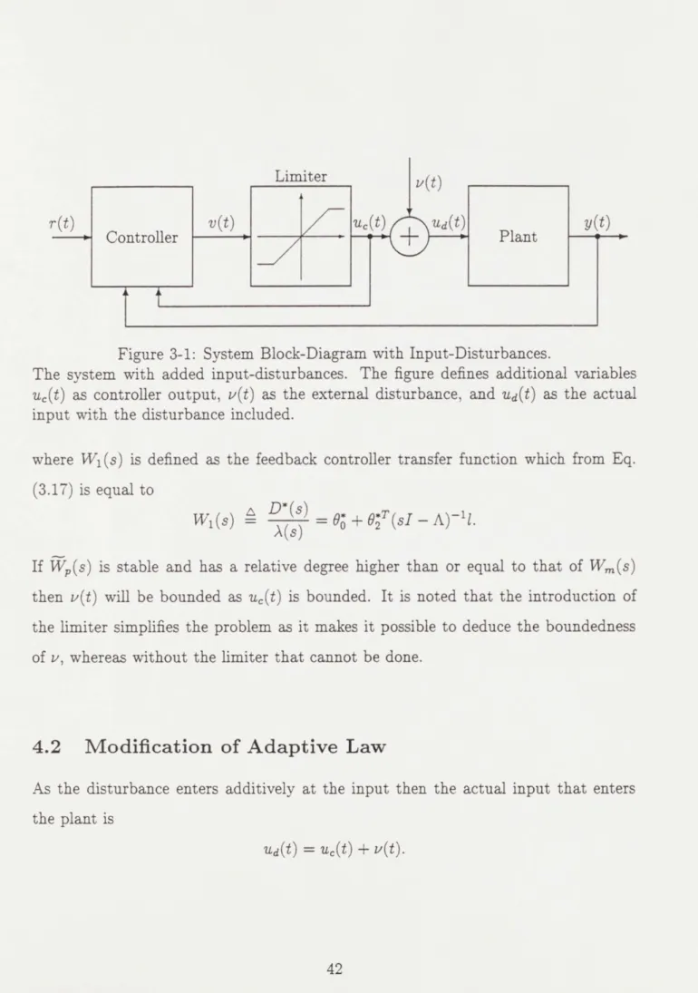
4.1 Disturbances . . . . 41

4.2 Modification of Adaptive Law . . . . 42

4.3 Stability . . . . 44

5. Sim ulations . . . . 45

5.1 1st Order System . . . . 45

5.2 Output Feedback, Relative degree 2 . . . . 45

4 Adaptive Control of Discrete-Time Systems 55 1. Model Reference Adaptive Control of a First Order Plant . . . . 55

1.1 Stability . . . . 57

2. One-Step-Ahead Adaptive Control of an nth Order Plant . . . . 58

2.1 Stability . . . . 60

3. Control in the presence of Bounded Disturbances . . . . 62

4. Sim ulations . . . . 64

4.1 Model Reference Control of a 1st Order System . . . . 64

4.2 One-Step-Ahead Control of a 2nd Order System . . . . 65

5 Application of Bounded Input Adaptive Control 75 1. Compliant Fingerpads . . . . 76

1.1 Computational Theory of Haptics . . . . 77

2. Dynamic Model . . . . 78

2.1 Constraints . . . . 81

2.2 Satisfaction of Constraints . . . . 81

3. Control Design . . . . 83

3.1 An Adaptive Controller . . . . 83

6 Summary and Conclusions 87 1. Sum m ary . . . . 87

2. Conclusions . . . . 87

Proof of Theorem 3.1 Proof of Theorem 3.2 Proof of Theorem 3.3 Proof of Theorem 3.4

B Proofs for Theorems in 1. Lemma B.1 . . . . . 2. Proof of Theorem 4.1 3. Proof of Theorem 4.2 4. Proof of Theorem 4.3 Chapter 4 1. 2. 3. 4. 89 91 94 96 100 100 101 104 107

2-1 System Block-Diagram . . . .

3-1 System Block-Diagram with Input-Disturbances. . . . .

3-2 Case (a) for Adaptive Control of a 1st-order Continuous-Time Plant.

Adaptive Adaptive Adaptive Adaptive Adaptive Adaptive Adaptive Adaptive Adaptive Adaptive Adaptive Control of a 1st-order Control of a 1st-order Control of a 1st-order Control of a 2nd-order Control of a 2nd-order Control of a 2nd-order Control of a 2nd-order Control Control Control Control Continuous-Time Plant. Continuous-Time Plant. Continuous-Time Plant. Continuous-Time Plant. Continuous-Time Plant. Continuous-Time Plant. Continuous-Time Plant.

of a 1st-order Discrete-Time Plant. of a 1st-order Discrete-Time Plant. of a 1st-order Discrete-Time Plant. of a 1st-order Discrete-Time Plant.

One-Step-Ahead Adaptive Control of a Discrete-Time One-Step-Ahead Adaptive Control of a Discrete-Time (c) for One-Step-Ahead Adaptive Control of a Discrete-Time

(d) for One-Step-Ahead Adaptive Control of a Discrete-Time 3-3 3-4 3-5 3-6 3-7 3-8 3-9 4-1 4-2 4-3 4-4 4-5 4-6 17 42 47 48 49 50 51 52 53 54 67 68 69 70 71 72 73 74

5-1 A schematic diagram of the dynamic model. . . . . 86

List of Figures

Chapter 1

Introduction

One of the major problems that arises while controlling dynamic systems is the trade-off between reaching maximum performance and robustness while using only practi-cally realizable control inputs. Physical limitations dictate that hard limits be im-posed on the magnitude to avoid damage to or deterioration of the process. Therefore, any active input that is determined on-line should meet the desired control objectives while remaining within certain limits. Also, from an analytical point of view, there may be a need to maintain the process near the desired operating point in order to make a linear control design adequate. This may in turn force the input magnitude to lie within certain bounds.

For example consider two fingers pinch grasping an object and moving it between two points. If both the fingers and the object are compliant then the dynamic charac-teristics of either one (such as stiffness and damping) influence the compressive force exerted by the fingers on the object. Also, the size of the contact area changes with the applied compressive force which in turn may affect the stability of the grasp. If the object is not to get dropped during manipulation the contact forces must be in compression at all times and the control signals must therefore be constrained to only those that produce compression between the object and both the fingers. Typically, the dynamic characteristics mentioned above are unknown and will vary with different grasp positions. This in turn means that some kind of adaptive control will be needed

exceed these bounds while simultaneously realizing the performance objectives is a very important problem.

Over the years, adaptive control methods have been developed to control systems that are poorly known. In particular, parametric uncertainties in linear dynamic systems have been effectively dealt with using adaptive control. Stability as well as robustness issues of adaptively controlling linear time-invariant plants with unknown parameters are well understood and documented in several textbooks and papers

[1, 2, 3]. The focus in all these cases has been on determining the least restrictive

conditions on the plant under which a control input can be realized to meet various control objectives. There was however no restriction on the magnitude of the control input, which commonly is the case as described in the last paragraph. In this thesis this problem of adaptive control with constrained input will be addressed and new methods and algorithms will be proposed to meet the constraints as well as the control objectives.

Chapter 2 describes how limits on the input amplitude affect the performance and stability of linear systems with emphasis on adaptive control. A review of the existing literature on adaptive control with input constraints is also given.

In Chapter 3 and 4, some new results on the problems described in chapter 2 are stated in Theorems 3.1-3.4 in Chapter 3, and 4.1-4.3 in Chapter 2. There modified control schemes and the stability of the overall system is established and results supported by simulations studies.

Chapter 4 describes an application of the results in Chapter 3. A simplified model of compliant fingerpads is analyzed and it is shown how the control of this model can be represented in the framework of constrained adaptive control.

1.

Constraints in Automatic Control

Control with constraints on the available control amplitude commonly occurs and is usually described as a linear plant with a nonlinear element describing the constraint, between the controller and the plant. Classical control theory does not have any

general tools or methods for the treatment of input non-linearities that are readily applicable to input saturation. This is especially true in the case of unstable systems where stability becomes naturally a primary concern if only a limited range of control values is allowed for whatever reason. Then the instability demanding large stabilizing inputs conflicts with the bounds on the input and a well founded stability theory is needed for the control design.

There has been considerable work done in the area of nonlinear systems stability [4, 5, 6]. While they are applicable and quite useful for specific classes of nonlinear systems they are inadequate for our purpose of determining conditions under which a linear time-invariant plant can be controlled inside a frame of input constraints. For instance, Describing Function Analysis consists of replacing a nonlinear element within the system with a specifically constructed linear element and then analyzing the resulting system. It is an approximate method and subject to some assumptions about the system and the nonlinearity and is mostly useful to predict the onset of limit-cycles and related phenomena. One can easily construct a description function for a hard-saturation but the assumptions made are too restrictive to be applicable to adaptive systems with any certainty. The Lure Problem refers to the control of a system whose forward path is linear and has a sector nonlinearity in the feedback path. Although hard saturation is, strictly speaking, not a sector nonlinearity, some of the many solutions developed for the Lure problem have included treatment of hard-saturation and time-varying nonlinearity [7, 5, 4] but they generally do not explicitly address unstable systems. Popov's Criterion is a solution to a specific case of Lure Problem and gives a condition for systems, which include sector nonlinearities, similar to what Nyquist's criterion gives for linear systems, leading to a condition in the frequency domain. Since it does not treat non-autonomous systems, it is not of use here. The Circle Criterion [8, 9] and [7, 10] is a more generalized version of

Nyquist's Criterion than Popov's Criterion. It can be extended to non-autonomous

systems, but like all the methods above the results are interpreted in the frequency domain and hence the result is obtained in global terms. That is, the question if the

that, this approach is inadequate for unstable systems with hard-saturation as they can only be locally stable. None of these methods directly addresses the stability of non-autonomous systems with time-varying linear feedback and hard saturation in the feed-forward path, which is the case for adaptive control with saturation. Finally, one important fact from the viewpoint of design is to have conditions that show what factors affect stability and in what way they do so.

1.1

Stability of Input-Constrained Systems

As the main focus of this thesis is on the stability properties of systems with input saturation some of the general stability properties of such systems are stated below. The system considered consists of a linear time-invariant, single-input plant and a controller when there is a hard limit on the amplitude of the command signal going from the control to the plant, (see Fig. 1.) Although this is a fairly general, structure it has some important properties, which are simply stated here but detailed and explained further in chapter 2.

Open-Loop Stable Plants

* In a system with a Bounded-Input, Bounded-Output stable (BIBO) plant, the plant can not be made unstable by any controller when there is a limit on the control signal. In such a case the input is always bounded and therefore the plant variables remain bounded.

* Then the stability of the controller is all that remains to be shown to ensure the stability of the overall system

Open-Loop Unstable Plants

* If the plant is strictly unstable then there exists an initial condition for the plant so that the system is unstable for all subsequent control inputs. This fact becomes obvious if the plant is considered in state description of Jordan form. Therefore the system can only be shown to be stable when the initial conditions

are within a compact set, which forms a stabilizable region in the state-space, i.e. locally stable.

" It can also be shown that there exist a bounded reference input which can drive

the plant out of the stabilizable region for a fairly general class of controllers. Therefore one can not show stability for all finite reference trajectories but only for those that remain within some bounds. Hence, one of the quantities that need to be determined for stability are these bounds.

" If an adaptive controller is used in addition to the above mentioned bounds,

the initial condition of the control parameter must be bounded as well, since in that case the control parameter is also a part of the system state. Initial values outside these bounds could drive the plant into instability.

Having these facts in mind, it is clear that stability for an adaptive system with hard saturation is local and the condition must depend in some way on all the factors detailed above.

2.

Adaptive Control with Limits on the Input

Amplitude

Adaptive control is no exception from other control methods in that large input am-plitudes must frequently be constrained, although in classical adaptive control theory it is generally assumed that unlimited amplitude is available. Still, if not intention-ally avoided, it typicintention-ally results in high control signals which cannot be implemented

by actuators in practice. One possible way to avoid this is to penalize the control

input amplitude in some way and methods for that have been developed [3]. Penal-izing the control amplitude results in lower amplitudes but does not give any insight into, whether the system will be stable or not. For direct adaptive control of stable discrete-time plants the effect of saturation is not very serious if good care is taken,

provided that the saturation bounds are known [3]. This is not true for continuous-time systems and algorithms will not work correctly unmodified. A basic structure for modifying the continuous-time adaptive law for effects of saturation limits was proposed by Monopoli in 1975 [11] but no stability proof was provided in this paper. Much of this thesis will be on showing how these algorithms need to be modified.

3.

New Results

The new results that this thesis contains are in the area of adaptive control of linear time-invariant, SISO plants with input constraints, and are in two parts.

New algorithms for continuous-time systems which ensure that parameters are es-timated correctly with saturation, are put forward for the most common cases. That includes, for first-order plants, states-accessible plants, relative-degree equal one, and plants of relative degree two and greater. In all cases the results are restricted to minimum-phase plants as when the control is unconstrained. Stability theorems are proved for all the algorithms above and also for two

pro-totype cases of discrete-time plants, i.e. for model reference adaptive control of first-order plants and for one-step-ahead direct adaptive control for plants of arbitrary known order.

4.

Application of Constrained Adaptive Control

As stated earlier in this chapter, manipulation problems with pinch finger grasp typ-ically lead to control with input constraints. Then the mathematical model is based on the assumption that friction between the two surfaces in each contact prevents slip. This assumption can only be true if the contact force is compressive and results in sufficient pressure in the contact area to counteract tangential forces. If the finger-pads and the object are assumed to be compliant the complexity increases since the interaction is dynamic and possibly unknown. The reason for exploring this problem

is to understand what principles lie behind successful completion of robotic tasks in manufacturing which involve mechanical interactions between the robot and its envi-ronment. Examples of such tasks are drilling, grinding, inserting a peg-in-a-hole, and assembly operations. Also, for general purpose robots that need to explore and ma-nipulate objects in their environment, the presence of compliance in the end-effector and explicit modeling of it is desirable for many reasons. The ones that come readily to mind are:

" Compliant fingers an object will generally have a finite area of contact, in

con-trast to point contact as is the case when the fingers and the object are assumed to be rigid. The introduction of a finite area of contact gives more stable grasp for fewer fingers as then additional resisting and stabilizing torsional torque ap-pears, which resists rotation around normal to the contact area. The effects of this additional torque can well be seen from the fact that the minimum number of finger contacts to ensure a stable grasp decreases from two to three when the finite are of contact is introduced.

* The stresses resulting in the contact region will be much less in the compliant case as the total force is distributed over the area of contact and not concen-trated as in the case of a point contact. This leads to increased dexterity as more fragile objects can then be manipulated.

* Exact shape of the object in the contact region will be less important for stability in the compliant case and not as crucial as in the rigid case.

* The explicit modeling of the compliance in the finger and the object will lead to dynamic models of higher order, which to some extent provides increased maneuverability as then the control bandwidth can possibly be increased. Often, as in the case of a general purpose robot, the objects encountered can possess a wide range of dynamic characteristics. This implies that the grasping and

question is unknown. In such cases, the control forces on the fingerpads need to be generated using an adaptive rather than a fixed controller.

The general problem of contact between two deformable bodies leads to a spatio-temporal analysis. Here, the problem will be simplified by adopting single degree-of-freedom lumped parameter model, thus reducing the variables to be purely temporal. The fingers as well as the object are assumed to deform only in one direction. The aim will be able to hold a compliant object with unknown dynamic parameters in a two-finger pinch grasp and move it along any desired path in a three-dimensional, gravity environment, while ensuring that the object does not slip or get crushed.

Because the system essentially describes a motion in free air, the resulting model is unstable, having a double integrator. This is the problem that motivated the work on the control algorithms and stability theorems in this thesis. The results obtained are however applicable to a more general class of problems and form the main subject.

Chapter 2

Overview

1.

Constraints in Automatic Control

Control amplitude1 saturation is often the dominant nonlinearity in control design although there is very little formal theory that addresses it [14]. In the literature, the main emphasis has been on providing schemes that preserve linear behavior under saturation, if possible, and otherwise provide graceful degradation of system perfor-mance under saturation. Several ad hoc schemes have been proposed [14, 15, 12, 16], along with others which are analytically more rigorous [17, 18]. The former schemes are, first and foremost, intended to prevent integrator windup resulting from satura-tion, but [17] is concentrated on preserving the properties of a linear time-invariant MIMO control design. None of the above schemes is much concerned with the domain of stability for unstable plants except for [18], which discusses the problem but does not give any explicit results on stability. The size of domain of stability is treated for systems with linear feedback in [5, 19, 20], where the approach is to maximize the domain of stability using numerical search methods.

'Control input is most often considered to be limited only in the amplitude but a more realistic approach would be to also include a limit on the rate of the control input [12, 13]. In this thesis, only amplitude constraints will be treated.

2.

Functional or State Constraints

Input constraints have several implications on the dynamic model and the control design. For instance, they may imply that the mathematical model used is only valid for a certain region of the state space. The region may be where linearity is preserved or where some functioning constraint must be satisfied. The region will be described

by some constraint function of the state variables. When carrying out the control

design, these constraints may limit the possible reference inputs as well as how the feedback signal is used in the control signal. The combined effect of these is then limited by intentionally restricting the control amplitude to a certain range. Making some assumptions on the frequency content of signals involved and using the limits obtained from the transfer function from the input to the output variable describing the constraint, the limits on the input can be projected to a range in the constraint variable.

3.

Stability of Input Constrained Systems

Now some general stability properties of systems which consist of a single-input, linear time-invariant plant and a controller with a hard limit on the amplitude of the command signal going from the controller to the plant (see Fig. 2-1). Some of the results are independent of the structure of the controller, but in each case where that is not true the assumed structure will be detailed with the result.

Stable Plants

A linear time-invariant (LTI) plant which has a hard limit on the control input and is

itself strictly open-loop stable, will always remain stable as in the linear case stability and bounded-input bounded output (BIBO) stability are equivalent [1]. The stability of the controller is then the only thing that needs to been ensured. If the controller has a integrator (e.g. a PID controller) then special care has to be taken and the danger of instability is a commonly known problem usually called Integrator windup.

Limiter

r(t) v(t) u(t) y(t)

- Controller - +-- Plant

Figure 2-1: System Block-Diagram

The system that this section is devoted to investigate. The figure defines variables

r(t) as the reference input, v(t) the control signal before saturation, u(t) the control

signal after saturation and y(t) as the plant output

The results of [15, 14, 16] suggest control schemes which can overcome this problem.

Plants with multiple integrators

If the plant has in it a higher order integrators but is otherwise stable, the problem of stability becomes more complicated. However results for continuous-time plants exist that give globally stabilizing controllers with bounded control amplitude, using nonlinear feedback [21]. It can further be shown that a saturating linear time-invariant feedback control, cannot possibly globally stabilize a plant with integrators of order greater than or equal to 3 [22].

Unstable Plants

If the plant is strictly unstable, i.e. having at least one unstable pole, some important facts can be stated about the stability of the system. A clear statement of these facts cannot been found in the literature. They will therefore be stated and proved here as Lemma 1 and 2. The first result is independent of what controller is used so the

Let a linear, time-invariant plant have a state-space description given by

(t) = Ax(t) + bu(t)

Iu(t)

and assume that it is of Jordan form, with a diagonal matrix A E R"' . The following lemma states that if the system in Eq. (2.1) is unstable it cannot be globally stabilized using any bounded control input.

Lemma 2.1 There exist a constant xm. and an initial condition x(to), both of which

are finite, with

I|x(to)I

solutions.

Proof:

Let A, be the eigenvalue of A for

j

Ai ₂ Re(Aj) V j = 1, 2,...n. (2.2)

Since A is in a diagonal form, the equation corresponding to the eigenvalue Ai can be written as

i(t) = Aixi(t) + biu(t). Since A is unstable , Ai > 0. It follows that

1 d

1 d (t) = _{Airx(t) + xi(t)biu(t)}

2 dt"

* Ai

1xi(t)1

_Ixi(t)I

> 0 V

Ixi(t)|

I

where

xm" = IbitUmx (2.4)

the unitary state transform T == 2)

7]

1and

Then the state-space spanned by the eigenvectors corresponding to these two eigen-values satisfy the equation

X~t) = pilp + WiJp + OU(t) J=,

.- 1 0

p and 0 are real, I is the identy matrix and pLL and wi denote, respectively, the real and the imaginary parts of A2. This gives the relation

1

g||p(t)jj

IIp(t)II

From Eq. (2.4) and (2.5) it is notes that a constant xma exists satisfying the condi-tions stated in Lemma 2.1 and hence the proof.

Now it will be shown that a bounded reference input, r(t) can be found for which a feedback controller destabilizes the system defined in Fig. (2-1) and Eq. (2.1)

Let the feedback controller be described by

where

sup

f(x,

1*0li5X. 1fO(x't)1

and f and fo are such that condition giving existence of solutions are satisfied. Further assume that the system is controllable for all times. Then we have the following lemma.

Lemma 2.2 There exists a bounded reference trajectory that destabilizes the plant in

Eq. (2.1) with the controller structure in Eq. (2.7) satisfying Eq. (2.8).

Proof: As in the proof of Lemma 2.1, assume that Ai, defined in Eq. (2.2) is real. If

r(t) = -f(x, t) + Ci- Ci > 0 (2.9)

fO(x,

then the control signals defined in Fig. 2-1 will be, u = v = ei for sufficiently small El. Also assume without loss of generality that x(to)

>

in

i (t) = Aix + ei > 0 Vt > to.

or xi(t) -+ oo as t -> oo. Hence , any reference input of the form in Eq. (2.9) drives the system into the unstable region. It is further noted from Eq. (2.8) that r(t) is bounded. 9 A similar proof can be given, even if Ai is complex.

It is worth noting that a special case of the controller in Eq. (2.7) is the linear feedback controller

v(t) = f (t) T x(t) + fo(t)r (t) which satisfies Eq. (2.8) if f(t) is bounded and fo(t) : 0.

Both Lemma 1 and 2 hold for discrete-time systems as well. The proofs are almost identical and are therefore omitted. For sake of completeness the discrete- time form of Lemma 2.1 will now be stated.

Lemma 2.3 (Discrete-time system) If the discrete-time system

is unstable, with Ad, defined as the eigenvalue of Ad E Ex, wzth the largest modulus,

JAd, 1. Also bd, defined as the entry in bd corresponding to Ad. Then there exist a

constant

s Ib,|um.

IAd- 1

and an initial condition p(to), both of which are finite, with ||V(to)II

>

the system has unbounded solutions.

4.

Adaptive Control with Limits on Input

Am-plitude

Most adaptive control algorithms that have been developed so far are for plants with a known structure but poorly known parameters. For linear plants this typically

means that the order, and the relative order of the plant's transfer function are known but its coefficients are unknown. Further a distinction is made between direct and indirect adaptive control. Indirect control refers to that an intermediate step is taken, in estimating explicitly the plant parameters to be used to calculate the control parameters, whereas in direct adaptive control this step is omitted and the control

parameters are estimated directly. Although both these approaches are equally valid, only the case of direct adaptive control will be treated in this thesis.

In direct adaptive control, the parameters of the controller are adapted over time,

in principle, based on a comparison of the expected and the resulting plant output. The rule for the adjustment of the parameter is expressed as an adaptive law, usually in the form of a differential equation for continuous-time systems and a difference equation for discrete-time systems. The state of the overall system will therefore contain the time-varying parameters of the controller in addition to the plant and other controller states. The system state space will then necessarily be composed of linear and nonlinear subsystems which makes the overall system nonlinear and time-varying. For continuous systems the controller and the adaptive law take the

form

v(t) = 9T(t)x(t)+r (t)r(t)

= 9T

(t)W(t)

u(t) =

{t

Umaxsgn(V(t)) if

Iv(t)I

where x(t) is the system state or the output from a state estimator,

w(t) = xT(t), r(t)]T and 9(t) =

[(t),

The function

fc(-)

For the discrete-time case the controller structure is

v(t) = ii(t)pV(t) + Ou(t) + Or(t)r(t)

= OT(t)p(t)

(t)

{

Umasgn(v(t)) if

Iv(t)I

Here p, and p contain a measurement history of the plant output, y(t) and the

_ 9 9'T 9 an L [VT T' ~,]. As in

control input, u(t),respectively, = , 7 , I, and o

[

the continuous-time case, the function fd(-) stands for an adaptive law of some form. Here V plays the role a state vector in a nonminimal state-representation of the plant. For continuous-time systems, the introduction of a limiter seriously affects the adaptive law in a way which is not trivially compensated for. In [11] Monopoli proposed the addition of correcting signals in the adaptive law. The treatment is however, not complete and not quite rigorous in view of the advances in the field since then.

Discrete-time systems on the other hand , do not need any modifications in the adaptive law; standard adaptive laws naturally accommodate saturation effects [3].

In both cases of continuous and discrete-time controi. a knowiedge of the actuai control signal amplitude, u(t) , i.e. the control signal after saturation is needed. When the measurement is not available, the saturator can be implemented inside the controller, hence effectively moving the saturator inside the controller. A lower bound on the actual, external saturation limit must then be known.

4.1

Stability of Adaptive Systems with a Saturated Input

The presence of a limiter ensures bounded inputs. This implies that if the plant is stable, all the state-variables of the plants are bounded. All that remains to be shown is that the signals in the controller remain bounded. In most cases, this boils down to proving the boundedness of the control parameter. For unstable plants, the problem becomes more complicated. It should be noted that the results of Lemmas 2.1 and 2.2 are applicable in this case.

Lemma 1 is applicable to any unstable system with a LTI plant and is therefore valid in that case here. It is also noted that the controller structure is the same as is assumed for Lemma 2, although it is too early to say whether the other conditions of Lemma 2 are satisfied.

Continuous-Time Constrained Adaptive Control

In continuous-time adaptive control, the general approach is to construct a reference

model which describes the desired behavior of the closed-loop system and would be

implemented if all the plant parameters were perfectly known. The fundamental assumption made is that a nominal value for the control parameter, 0 = 9* exists for

which the system behaves exactly like the reference model. This is one of the reason behind the restriction that the structure of the plant must known, as it can argued that a knowledge of the structure is necessary to make the plant behave identically to the model by merely choosing the right control parameter. This control parameter is what the adaptive law is designed to search for. It is not guaranteed, although, that

given a sufficiently -rich" set of reference inputs2 then the control parameter estimate will converge to the correct value. That the parameter vector is a part of state for the overall system suggests, in view of Lemma 1, that the initial conditions for that parameter vector must also be bounded. This is indeed the case as will be stated in the following lemma. Let

fc(-)

IIfc(w,

when t, and w are bounded.

Lemma 2.4 If the controller structure in Eq. (2.11) satisfying Eq. (2.13) is used for

system (2.1) then there exists a finite 9(to) such that the origin of the linear subsystem is unstable.

Proof: Instability means that there exists a point, in the linear subsystem, arbitrarily close to the origin and a bounded initial condition for the control parameter that lead to unbounded trajectories.

As in the proofs for Lemmas 2.1 and 2.2, consider the most unstable eigenvalue,

Ai of the linear subsystem, and the corresponding decoupled, differential equation

i(t) = Aix1(t) + biu(t)

Without loss of generality assume bi > 0 and let xi (to) = exm,, where 0 < e < 1 and xm, is defined in (2.4). Let C and j be the the state vector and the parameter vector, respectively, obtained by excluding the entries corresponding to xi from w and

9. The system is linear and in view of Lemma (2.2) only bounded reference inputs

are considered, then 3-y, cl, co > 0 such that

II&(t)I

2_{The signals that satisfy this richness condition are referred to as persistently exciting in adaptive}

Fma(t, to) sup Fe(w, r), to <T<t

then if j(to) = 0 it follows that

j|(t)|

and by choosing

9

Cxmax _I

tu =L to + 1 log

u(t) = F(t)&(t) _{+ Oi(t)xi(t)}

-&max(t - t₀)F~m(t, to)(t - to) + (9,(to) - Fmx(t, to)(t - to)) X,(t),

(2.14) giving u(to) 0, so i(to) is increasing and because Eq. (2.14) holds for all x2(t) >

CXmax when to < t < tu, it follows that

.j(t) = Aix(t) + biu(t)

> Aix(t) Vt E [totu]

and

xi(tu) exmaxe *~o) = Xmax

and from Lemma 2.1, the proof follows.

As before with Lemmas 2.1 and 2.1, Lemma 2.4 applies equally to discrete-time systems.

Let

where

4.2 Conclusion

The following conclusions can be drawn from Lemmas 2.1, 2.2 and 2.4.

To guarantee stability for an adaptive system as described in Eqns. (2.1), (2.3) and (2.11) where the plant is not necessarily stable the following factors must be included.

1. A bound on the initial conditions of the plant.

2. A bound on the magnitude of the reference input.

3. A bound on the initial conditions of the parameter estimate.

Exactly how these factors contribute to stability will be the main subject of chap-ters 3 and 4.

5.

Papers Published on Adaptive Control in the

Presence of Constraints

As stated before, the basic structure for modifying the adaptive law for effects of saturation limits was proposed by Monopoli in 1975 [11]. Papers that have dealt with this problem in the past few years include [23] -[31]. In [23]-[29] it is assumed that the plant is open-loop stable. In [24, 25] the problem of discrete time, direct adaptive control is addressed In [27]-[30] the problem of discrete time, adaptive pole-placement control is addressed and by and large all employ projection to guarantee bounded parameter estimates and based on that derive global stability for type-1 plants. In [29] the case of continuous time indirect adaptive control is explored and there again projection is used in the adaptive algorithm and stability results only for open-loop stable plants given. In [31] the proposed approach of Monopoli in [11] is followed in continuous time direct adaptive control, i.e. to modify the adaptive law by augmenting the error signal with correcting signals to establish parameter boundedness as before results apply only to open-loop stable plants.

Chapter 3

Adaptive Control of

Continuous-Time Systems

In this chapter some new results obtained on the problems described in the previous chapter are stated in Theorems 3.1-3.4 where modified control schemes and stability of the overall system is established. Simulations are presented to support the theoretical derivations.

1.

A First-Order Plant

Statement of the Problem: A plant with an input-output pair {u(.), x,(.)} is

described by the scalar equation

i,(t) = apx,(t) + bpu(t) (3.1)

where a, and b, are unknown, but the sign of b, is assumed to be known. The input u(t) is additionally subject to the magnitude constraint

u(t)I

A reference model is described by the first-order differential equation

im(t) = amxm(t) + bmr(t) (3.2)

where am is a known negative constant, bm is known, and r(t) is a piecewise-continuous bounded function whose magnitude is such that

Ir(t)I ro.

It is assumed that am, bm and r(t) have been chosen so that xm(t) represents the output desired of the plant at time t. The aim is to determine a bounded control input u(t) so that all signals in the system remain bounded, for a given set of initial

conditions, and x, tracks xm as closely as possible.

If the plant parameter is known, a feedback controller of the form

u(t) = 9*xp(t) + k*r(t), where 0* = am- ap and k* bm

suffices. Since a,, b, and hence 0*, k* are unknown the control input is chosen to have the form

v(t) = 0(t)xp(t) + k(t)r(t)

(t) v(t) if Iv(t)I uO

(3.3)

uosgn(v(t)) if

Iv(t)I

where 9(t) is a time-varying control parameter. Then the closed-loop system can be described by

6,(t) = (a, + b,(t))x,(t) + bAu(t) + bpk(t)r(t) (3.4)

where Au(t) = u(t) - v(t). If the output error e(t) and the parameter errors

#(t)

the obtained error equation is from Eqs. (3.2) and (3.4) as

6(t) = ame(t) + bpk(t)xp(t) + bO(t)r(t) + bpAu(t).

In order to remove the effect of Au, which can be considered as a known disturbance, a signal e&(t) is generated as the output of a differential equation

da(t) = amea(t) + ka(t)Au(t) eA(to) = 0.

If e,.(t) = e(t) - eA(t), it is obtained that

du(t) = ameu(t) + bpo(t)xp(t) + bppr(t) + (t)Au(t). _(3.5)

Where x(t) = bp - ka(t). Eq. (3.5) is in a standard error model form for which the

following adaptive laws can be used

#(t) = -Y 1sgn(b,)eux,

(t) -7y 2sgn(b,)eur (3.6)

k(t) = -Y ₃euAu

where -y > 0 i = 1, 2, 3. This results in a Lyapunov function

1

r

2

V = - [e2 +

lb,

2 .U ₇₁ + ₎₇₃ -K2]_. (3.7)

since V = ame2 < 0. Hence 0(t), V)(t), ,c(t) and eu(t) are bounded Vt

>

it can be deduced that 3 4m, < oo such that

I0(t)

I

IV(t) I

to, where

71

(3.8) Theorem 3.1 The adaptive system in Eqs. (3.1), (3.2), (3.3), and (3.6) has bounded

solutions V jr t)j < To if

b~o j&T|am| - k*! J a,|

(i)

IxP(to)I

II

Further,

IxP(t)

a,

Proof: See Appendix A

Theorem 1 implies that adaptive control of a first-order plant in Eq. (3.1) leads to bounded solutions with the controller in Eq. (3.3) and the adaptive law in Eq.

(3.6) provided conditions (i) and (ii) are met. The boundedness of all signals in

the adaptive system was established in two steps. First the parameter error 0(-) was shown to be bounded which was done using the adaptive law in (3.6). Next the boundedness of the state x, of the plant was derived, if the initial conditions are restricted to remain within a bounded set. Additional comments regarding the bounds on the initial conditions are made at the end of section 2..

2.

State Variables Accessible

In this section the plant considered is an nth order one, whose states are accessible and described by the vector differential equation

,(t) = Ax,(t) + bu(t) (3.10)

where the entries A,, E RnL and b, E R are unknown. It is assumed that a reference model described by

m(t) = Amxm(t) + bmr(t) (3.11)

can be determined where r(t) is a piecewise-continuous bounded function with

Ir(t)

I<

0* and a scalar k* exists and are solutions of

Ap+b m*T = Am

k*b, = b,.

As in the scalar case the, input u(t) is subjected to the magnitude constraint

Iu(t)I uo

where uo is a known constant. The aim is to determine a bounded control input

u(t) so that x, tracks xm as closely as possible while all signals in the system remain

bounded. The main result is summarized in the following theorem. Theorem 3.2 Let an adaptive controller be chosen as

v(t) = k(t)9T(t)xp(t) + k(t)r(t)

u(t) = v(t) if |v(t)| UO

uosgn(v(t)) if

Iv(t)I

= -xeTPbm (3.12)

= -71lueTPbm

6a (t) = Amea(t) + bmk(t)-'Au(t) eA(to) =

0

eu(t) e(t) - e(t) #(t) =0 (t) - *(t) V)(t)

-k* k t )

where Ap + PAm =-Q and

Q

IIPbm||

1

V(eu, #, 0) = eTPeu + #Tr-~o+ -v)2 r = r > o -Y1 > 0

then the adaptive system in Eq. (3.10) has bounded solutions if

(i) xT(to)Px(to) < Amin(P)

k*I|

_*I-

_2o

3 .1 3 )

1 qo - p jk*| !A |2Pb||6*|| - go|

and (ii) V(to) < (.

Aa.x(Tr) 2Pb + a k*| [ q + 2Pb h6* M

Further,

xT(t)Pxp(t) < Amin(P)|k*||2pbII* - goi V t > to. (3.14)

Proof: See Appendix A

Remarks:

1. Theorems 3.1 and 3.2 imply that if the initial conditions of the state as well as the parameter error lie within a certain bound, then the adaptive system will have bounded solutions. The local nature of the stability result is to be expected

in view of Lemmas 2.1-2.4, since the control input was restricted to lie within certain limits. This condition can only be removed by restricting the open-loop poles to lie in the left half plane. Theorems 3.1-3.4 extend this statement to the

adaptive case, where the control parameter is also a state-variable of the overall

nonlinear system, and hence requires not only a bound on

I|x(to)I

the norm of the parameter error I(to) .

2. Condition (ii) implies that prior information regarding an upper bound on 110*|1

needs to be known so that the matrix Q and hence qo can be chosen to make the

right hand side in condition (ii) positive. Since the feedback control input has a

component due to the external input and a component due to the plant-model mismatch, it is not surprising that for a given parameter I 1* 1, the scaling factor

ro/uo must be small. That is, the magnitude of the reference input r(t) and,

hence, of the state of the model xm that the plant state must track, must be appropriately scaled. As the mismatch between the plant and the model gets reduced, the factor ro/uo can be increased.

3. It should be noted that the adaptive algorithm in Eq. (3.12) leads to the boundedness of the control parameter 0. Since the plant input u is always bounded, this implies that if the plant is open-loop stable, the boundedness of the remaining signals in the closed-loop system immediately follows, without any restriction on the initial conditions of the plant or the controller, leading to global stability. Conditions (i) and (ii) in Theorems 3.1 and 3.2 are therefore required only for unstable plants.

4. It is interesting to note that the results will hold for any adaptive law which guarantees boundedness of the parameter error and will therefore extend to the algorithms proposed in [31] as well.

3.

Output Feedback

Now a look will be taken at the case when only the output is available for feedback. The plant considered is single-input single-output system described by

,(t) = Apx,(t) + bpu(t) y,(t) = h x,(t) (3.15)

where the input u is subjected to the constraint

Iu(t)I <; uo Vt > to,

and xP : R+ -+ R' is the n-dimensional state vector of the plant. Eq. (3.15) is

written equivalently as a transfer function

W,(s) = kZ(s) = h T(sI - A,)-1b,

R,(s) P

where Z,(s) and F,(s) are monic polynomials in the differential operator s. The following standard assumptions are made regarding W,(s):

2. An upper bound, (n), on the order of the plant is known.

3. The relative degree, (n*), of the plant is known.

4. The roots of Z,(s) are known to be in the open left half of the complex plane, i.e. Z,(s) is Hurwitz.

5. The system {h,', A,, b,} is controllable and observable.

The objective is to let the plant output y,(t) follow a reference trajectory ym (t) as closely as possible. To achieve that a a reference model is introduced, described

by a linear time-invariant, asymptotically stable system with an input-output pair

{r(-), ym(-)}, and described by a transfer function

Win(s) = km (S)

Rm(s)

with a relative degree n*, > n*, where Zm(s) and R,(s) are monic polynomials in the

differential operator s, and km is assumed to be positive. The reference input r(t) is

assumed to be a uniformly bounded piecewise-continuous function of time, and that

Ir(t)I ro V t > to.

Similar to the standard adaptive controller in [1], a controller is chosen of the form

,(t) = Awi(t) + lu(t) 2 (t) = Aw2(t) + ly,(t) W (t) = r(t), L4)1(t), y,(t), Uo2(t)] O(t) = [k(t),

9T(t),

OT(t)

{

Iv(t)I

Iv(t)I

where k : 11 -+ 0, L1 : Rli* ---+ R" 1, 00 : R - IR, 02, L ₂ : IR+- _ n- 1, A is

an asymptotically stable matrix and det(sI - A) = A(s). It follows that when the control parameters k(t), 01(t), 0 (t), 02(t) assume the constant values k,, 01c, 90c, 02c,

respectively, the transfer function of the feedforward and the feedback controllers become respectively

A(s) and D(s) (3.17)

A(s) - C(s) A(s)

where C(s) is determined by 01c and D(s) by 02c, 0oc or

C(s) = sI - A)-11, D(s) = 0Oc + OT (sI - A)-'I.

A(s) A(s) O L sI

The overall transfer function of the plant together with the controller can be expressed as

WO(s) = kekZ,(s)A(s) (3.18)

(A(s) - C(s))R,(s) - kZ,(s)D(s)

where ke - -. If we now chose A(s) so that it contains Zm(s) as a factor, A(s) =

Zm(s)Ai(s) then (3.18) becomes

WO(s) = kckpZp(s)Ai(s)Zm(s) (3.19)

(A(s) - C(s))R,(s) - kZ,(s)D(s)(

The existence of the control parameter 9*, which lets W (s) Wm (s), is equivalent

to the existence of the polynomials C*(s), D*(s), and the gain k* such that the denominator polynomial in Eq. (3.19) becomes Zp(s)Aj(s)Rm(s). Identifying R(s) with Q(s), -kpZ,(s) with P(s) and Zp(s)Aj(s)Rm(s) with Q*(s) the problem is to

determine C*(s) and D*(s) such that

[A(s) - C*(s)] Q(s) + D*(s)P(s) = Q*(s),

which is the Bezout's identity and it guarantees the existence of D*(s), and C*(s) if Q(s) and P(s) (or equivalently, R,(s) and Zp(s)) are relatively prime, i.e. the

solution to exist. The differential equation describing the plant together with the controller can be represented as

p(t) = Apxp(t) + bp(9(t)Tw(t) + Au(t))

L 1(t) = Awi(t) + 1(0(t)Tw(t) + Au(t))

2 (t) = Aw2(t) + l(hTx,)

(3.20)

where Au(t) = u(t) - v(t).

errors defined as

With the controller in Eq. (3.16), and the parameter

0

(t)

0o(t)

00*

(t) = k(t) - k*,

02 (t) =2 2(t) - 02,

the overall system becomes

(t) = AmnX(t) + bmn [#T(t)w(t) + k*r(t) + Au(t)]

where Au(t) = u(t) - v(t),

Amn = Ap + bp9 h, l1 h bpo*T A + 1 9*T 0 bpo*TP2 1 9*T A bmn = I 0

hmn = [hT, 0, 0 and x = IX, Wi, W2

-Since W0(s) = Wi(s) when 9(t) =_ * it follows that the reference model can be

described non-minimally by the (3n - 1)th order differential equation

mn(t ) = AmnXmn(t) + b

where xmn(t) = [X*(t), aU*(t), Ls(t)].

yM(t) = h T xrn(t)

The signals in xmn(t) can be considered as (3.21)

(3.22)

signals in the reference model corresponding to Xij) in the overall system. Hence, the error equation for the overall system may be expressed as

6(t) = Amne(t) + bn [dT(t)w(t) + Au(t)] , ei(t) = h Te(t).

If el = yp - ym, the error model is given by

ei(t) = Wm(s) [T(t)w(t)]

in the absence of the limiter. With the limiter, if Au = u - v, it can be shown in a

straightforward manner that

el(t) = Wm(s)

[kT(t)w(t)

In what follows, the cases n* = 1 and n* > 2 are treated separately to describe the adaptive law which establishes the boundedness of the parameter error. Once this is done, the boundedness of the rest of the state variables of the adaptive system for arbitrary n* is established in section 2.3.3.

3.1

Adaptive law n* = 1

As in the standard adaptive control problem, the adaptive law is considerably simpler when n* = 1 than when n* > 2 since in the former case Wm(s) can be made strictly positive real (SPR). The Au(t) term in Eq. (3.23) is compensated for by generating the signal

eA(t)

where kA(t) is a time-varying gain, adjusted according to an adaptive law that is to be determined. If a compensated error eu1 is defined as eu1 = el - e&, and a parameter

where

=U ['kA T(t)]T WU (t) = [AU(t), WT(t)] T

The error model is now have in a recognizable form, and hence an adaptive law can be found by inspection as

= -sgn(kp)Fwei ul = -k*-yseujAu where r = rT > 0 and ya > 0.

(3.24) It should be noted that the adaptive law in Eq. (3.24) is implementable since

kA

y-aeuAu. The use of Kalman-Yakubovich lemma then gives us that eul, 0, E **, with a Lyapunov function

TD 1 1

V(eu, , ,&) = e T + jk* 1r + y&k-2A

where eu is the state corresponding to the output eul.

3.2

Adaptive Law, n* > 2

Here, as in the standard adaptive control problem, an augmented error is used to determine the adaptive laws. First define the signal

ea(t) = kA(t)Wm(s)Au(t)

where kA(t) is a time-varying gain, to compensate for the term Au(t) in Eq. (3.23).

If eu, = el - e&, then

eui(t) = hWm(S) [4T(t)w(t)] + P(t)Wm(S)AU(t)

where VbA(t) = j; - kA(t). Then the auxiliary error and the augmented error are

determined as

e₂(t) = [TWm(s)I - Wm(S)OT(t)] w(t)

It folhows that

1,'

lu= eP(t)k(t) + #A(t)A(t) +

i

where (t) = W'(s)Iw(t), (a&t) = W.(s)Au(t), and 6(t) is an exponentially decaying

term due to initial conditions. The adaptive laws can be found by inspection as

=

0(t)

'tP(t)

which gives us that eu 1, 1, ka E COO with

1 [1 OI + 1, p 1 2

(, '01,#) = 4 + + - 'I

2 jk*| 71 1 -Y

as a Lyapunov function.

3.3 Boundedness of Signals

The results in sections 2.3.1 and 2.3.2 imply that adaptive laws can be found which imply that, for any relative degree,

11(t)II

in Eq. (3.21). Define P as the symmetric positive definite solution to Lyapunov equation, and p as the ratio between the maximum and the minimum eigenvalues of

P so that

APn+PAmm =

-Q

Amxa(P)

9(t)

Let qo = AminkQ) and pb = Mb / = L, , P = , I' and = [9T, 00, 9 ]T. If 0 I 0 C= hT 0 0_p 0 0 I

then & = Cx. Also, since 4 = k, Tj , we have

II

Ik(t)I

for all t > to. Now the main result will be stated, which proves the boundedness of all signals in the adaptive system.

Theorem 3.3 The system in Eq. (3.21) has bounded solutions if

(to)

qo

2pbIIO*TC||

-2|k*| Ama(I') pg

I2PbI||*TC

(3.25)

-- 2

(ii) xT(to)Px(to)

5

Uo

.2Pb||#*T C|| - go|

Further

r

XT_{(t)Px(t) 5 Amij(P) 2pbO Vt > to.} 2Pb||N*TC|| - qo I

Proof: See Appendix A.

It is noted that condition (ii) in Theorem 3.3 is quite difficult to check since the quantity on the right hand side requires a fair amount of knowledge of the plant parameters. It may be argued that the bounds on the initial conditions in (i) and (ii) establish the existence of such values for which the overall adaptive system is stable. However as is seen in the simulation results in the next section, these bounds are indeed conservative and the initial conditions can be increased further before instability occurs.