HAL Id: hal-01223119
https://hal.archives-ouvertes.fr/hal-01223119
Submitted on 2 Nov 2015
HAL is a multi-disciplinary open access
archive for the deposit and dissemination of
sci-entific research documents, whether they are
pub-lished or not. The documents may come from
teaching and research institutions in France or
abroad, or from public or private research centers.
L’archive ouverte pluridisciplinaire HAL, est
destinée au dépôt et à la diffusion de documents
scientifiques de niveau recherche, publiés ou non,
émanant des établissements d’enseignement et de
recherche français ou étrangers, des laboratoires
publics ou privés.
Davide Frey, Roy Friedman, Achour Mostefaoui, Matthieu Perrin, Michel
Raynal, François Taïani
To cite this version:
Davide Frey, Roy Friedman, Achour Mostefaoui, Matthieu Perrin, Michel Raynal, et al.. D.1.2 –
Modular quasi-causal data structures. [Research Report] D1.2, LINA-University of Nantes; IRISA.
2015. �hal-01223119�
ANR-13-INFR-0003
socioplug.univ-nantes.fr
data structures
Davide Frey
1,2
, Roy Friedman
7
, Achour Mostfaoui
3
, Matthieu Perrin
3
,
Michel Raynal
1,2,5,6
, Franois Taiani
1,2,4
1IRISA Rennes 2
Inria Rennes - Bretagne Atlantique
3LINA, Universit de Nantes 4Universit de Rennes 1 - ESIR 5
Universit de Rennes 1 - ISTIC
6Institut Universitaire de France 7
The Technion, Israel
Email contact: {davide.frey,michel.raynal,francois.taiani}@irisa.fr, [email protected], [email protected]
In large scale systems such as the Internet, replicating data is an essential feature in order to provide avail-ability and fault-tolerance. Attiya and Welch proved that using strong consistency criteria such as atomicity is costly as each operation may need an execution time linear with the latency of the communication net-work. Weaker consistency criteria like causal consistency and PRAM consistency do not ensure convergence. The different replicas are not guaranteed to converge towards a unique state. Eventual consistency guaran-tees that all replicas eventually converge when the participants stop updating. However, it fails to fully specify the semantics of the operations on shared objects and requires additional non-intuitive and error-prone distributed specification techniques. In addition existing consistency conditions are usually defined independently from the computing entities (nodes) that manipulate the replicated data; i.e., they do not take into account how computing entities might be linked to one another, or geographically distributed. In this deliverable, we address these issues with two novel contributions.
The first contribution proposes a notion of proximity graph between computing nodes. If two nodes are connected in this graph, their operations must satisfy a strong consistency condition, while the operations invoked by other nodes are allowed to satisfy a weaker condition. We use this graph to provide a generic approach to the hybridization of data consistency conditions into the same system. Based on this, we design a distributed algorithm based on this proximity graph, which combines sequential consistency and causal consistency (the resulting condition is called fisheye consistency).
The second contribution of this deliverable focuses on improving the limitations of eventual consistency. To this end, we formalize a new consistency criterion, called update consistency, that requires the state of a replicated object to be consistent with a linearization of all the updates. In other words, whereas atomicity imposes a linearization of all of the operations, this criterion imposes this only on updates. Consequently some read operations may return out-dated values. Update consistency is stronger than eventual consis-tency, so we can replace eventually consistent objects with update consistent ones in any program. Finally, we prove that update consistency is universal, in the sense that any object can be implemented under this criterion in a distributed system where any number of nodes may crash.
Keywords:Causal consistency, Sequential Consistency, Eventual Consistency, Scalability, Distributed Com-puter Systems
1
Introduction
Reliability of large scale systems is a big challenge when building massive distributed applica-tions over the Internet. At this scale, data replication is essential to ensure availability and fault-tolerance. In a perfect world, distributed objects should behave as if there is a unique physical shared object that evolves following the atomic operations issued by the participants†. This is the aim of strong consistency criteria such as linearizability and sequential consistency. These criteria serialize all the operations so that they look as if they happened sequentially, but they are costly to implement in message-passing systems. If one considers a distributed implementation of a shared register, the worst-case response time must be proportional to the latency of the network either for the reads or for the writes to be sequentially consistent [LS88] and for all the operations for linearizability [AW94]. This generalizes to many objects [AW94]. Moreover, the availability of the shared object cannot be ensured in asynchronous systems where more than a minority of the processes of a system may crash [ABD95]. In large modern distributed systems such as Amazon’s cloud, partitions do occur between data centers, as well as inside data centers [Vog08]. Moreover, it is economically unacceptable to sacrifice availability. The only solution is then to provide weaker consistency criteria. Several weak consistency criteria have been considered for modeling shared memory such as PRAM [LS88] or causality [ANB+95]. They expect the local
histories observed by each process to be plausible, regardless of the other processes. However, these criteria do not impose that the data eventually converges to a consistent state. Eventual con-sistency [Vog08] is another weak concon-sistency criterion which requires that when all the processes stop updating then all replicas eventually converge to the same state.
These weaker consistency models are not a desirable goal in themselves [AF92], but rather an unavoidable compromise to obtain acceptable performance and availability [AW94, Bre00, XSK+14]. These works try in general to minimize the violations of strong consistency, as these
create anomalies for programmers and users. They further emphasize the low probability of such violations in their real deployments [DHJ+07].
In this deliverable we therefore present two contributions that aim to improve the state of the art of consistency criteria for large-scale geo-replicated systems. The first contribution, published in [FTR15], consists of a hybrid consistency criterion that links the strength of data consistency with the proximity of the participating nodes. The second, published in [PMJ15], addresses the limitations of eventual consistency by precisely defining the nature of the converged state. Motivation and problem statement
Roadmap This deliverable consists of 7 sections. Section 2 introduces the definition of our first contribution, fisheye consistency. Then, Section 3 builds on top of this communication abstraction a distributed algorithm implementing this hybrid proximity-based data consistency condition. Section 4 introduces preliminary notions towards the definition of our second contribution. Sec-tion 5 defines the new update-consistency criterion. SecSec-tion 6 presents a generic construcSec-tion for any UQ-ADT object with a sequential specification. Finally, Section 7 concludes the document.
2
Fisheye Consistency
In spite of their benefits, the above consistency conditions generally ignore the relative “dis-tance” between nodes in the underlying “infrastructure”, where the notions of “dis“dis-tance” and “infrastructure” may be logical or physical, depending on the application. This is unfortunate as distributed systems must scale out and replication is becoming more common. In a geo-replicated system, the network latency and bandwidth connecting nearby servers is usually at least an order of magnitude better than what is obtained between remote servers. This means that the cost of maintaining strong consistency among nearby nodes becomes affordable compared to the overall network costs and latencies in the system.
Some production-grade systems acknowledge the importance of distance when enforcing con-sistency, and do propose consistency mechanisms based on node locations in a distributed sys-tem (e.g. whether nodes are located in the same or in different data-centers). Unfortunately these production-grade systems usually do not distinguish between semantics and implementa-tion. Rather, their consistency model is defined in operational terms, whose full implications can be difficult to grasp. In Cassandra [LM10], for instance, the application can specify for each operation the type of consistency guarantee it desires. For example, the constraints QUO-RUM and ALL require the involvement of a quorum of replicas and of all replicas, respectively; while LOCAL QUORUM is satisfied when a quorum of the local data center is contacted, and EACH QUORUM requires a quorum in each data center. These guarantees are defined by their implementation, but do not provide the programmer with a precise image of the consistency they deliver.
The need to take into account “distance” into consistency models, and the current lack of any formal underpinning to do so are exactly what motivates the hybridization of consistency tions that we propose in our work (which we call fisheye consistency). Fisheye consistency condi-tions provide strong guarantees only for operacondi-tions issued at nearby servers. In particular, there are many applications where one can expect that concurrent operations on the same objects are likely to be generated by geographically nearby nodes, e.g., due to business hours in different time zones, or because these objects represent localized information, etc. In such situations, a fisheye consistency condition would in fact provide global strong consistency at the cost of maintaining only locally strong consistency.
Consider for instance a node A that is “close” to a node B, but “far” from a node C, a causally consistent read/write register will offer the same (weak) guarantees to A on the operations of B, as on the operations of C. This may be suboptimal, as many applications could benefit from varying levels of consistency conditioned on “how far” nodes are from each other. Stated differently: a node can accept that “remote” changes only reach it with weak guarantees (e.g., because infor-mation takes time to travel), but it wants changes “close” to it to come with strong guarantees (as “local” changes might impact it more directly).
In this work, we propose to address this problem by integrating a notion of node proximity in the definition of data consistency. To that end, we formally define a new family of hybrid consis-tency models that links the strength of data consisconsis-tency with the proximity of the participating nodes. In our approach, a particular hybrid model takes as input a proximity graph, and two con-sistency conditions, taken from a set of totally ordered concon-sistency conditions, namely a strong one and a weaker one. A classical set of totally ordered conditions is the following one: lineariz-ability, sequential consistency, causal consistency, and PRAM-consistency [LS88]. Moreover, as already said, the notion of proximity can be geographical (cluster-based physical distribution of the nodes), or purely logical (as in some peer-to-peer systems).
The philosophy we advocate is related to that of Parallel Snapshot Isolation (PSI) proposed in [SPAL11]. PSI combines strong consistency (Snapshot Isolation) for transactions started at
nodes in the same site of a geo-replicated system, but only ensures causality among transactions started at different sites. In addition, PSI prevents write-write conflicts by preventing concurrent transactions with conflicting write sets, with the exception of commutable objects.
Although PSI and our work operate at different granularities (fisheye-consistency is expressed on individual operations, each accessing a single object, while PSI addresses general transactions), they both show the interest of consistency conditions in which nearby nodes enjoy stronger se-mantics than remote ones. In spite of this similitude, however, the family of consistency condi-tions we propose distinguishes itself from PSI in a number of key dimensions. First, PSI is a spe-cific condition while fisheye-consistency offers a general framework for defining multiple such conditions. PSI only distinguished between nodes at the same physical site and remote nodes, whereas fisheye-consistency accepts arbitrary proximity graphs, which can be physical or logical. Finally, the definition of PSI is given in [SPAL11] by a reference implementation, whereas fisheye-consistency is defined in functional terms as restrictions on the ordering of operations that can be seen by applications, independently of the implementation we propose. As a result, we believe that our formalism makes it easier for users to express and understand the semantics of a given consistency condition and to prove the correctness of a program written w.r.t. such a condition.
2.1
System Model
The system consists of n processes denoted p1, ..., pn. We note Π the set of all processes. Each
process is sequential and asynchronous. “Asynchronous” means that each process proceeds at its own speed, which is arbitrary, may vary with time, and remains always unknown to the other processes. Said differently, there is no notion of a global time that could be used by the processes. Processes communicate by sending and receiving messages through channels. Each channel is reliable (no message loss, duplication, creation, or corruption), and asynchronous (transit times are arbitrary but finite, and remain unknown to the processes). Each pair of processes is connected by a bi-directional channel.
2.1.1
Basic notions and definitions
This section is a short reminder of the fundamental notions typically used to define the consis-tency guarantees of distributed objects, namely, operation, history, partial order on operations, and history equivalence. Interested readers will find in-depth presentations of these notions in textbooks such as [AW04, HS08, Lyn96, Ray12].
Concurrent objects with sequential specification A concurrent object is an object that can be simultaneously accessed by different processes. At the application level the processes interact through concurrent objects [HS08, Ray12]. Each object is defined by a sequential specification, which is a set including all the correct sequences of operations and their results that can be applied to and obtained from the object. These sequences are called legal sequences.
Execution history The execution of a set of processes interacting through objects is captured by a history ̂H= (H,→H), where →His a partial order on the set H of the object operations invoked by
the processes.
Concurrency and sequential history If two operations are not ordered in a history, they are said to be concurrent. A history is said to be sequential if it does not include any concurrent operations. In this case, the partial order→His a total order.
Equivalent history Let ̂H∣p represent the projection of ̂Honto the process p, i.e., the restriction of ̂Hto operations occurring at process p. Two histories ̂H1and ̂H2are equivalent if no process can
distinguish them, i.e.,∀p ∈ Π ∶ ̂H1∣p = ̂H2∣p.
Legal history Ĥbeing a sequential history, let ̂H∣X represent the projection of ̂Honto the object X. A history ̂His legal if, for any object X, the sequence ̂H∣X belongs to the specification of X. Process Order Notice that since we assumed that processes are sequential, in the following, we restrict the discussion to execution histories ̂H for which for every process p, ̂H∣p is sequential. This total order is also called the process order for p.
2.2
The Family of Fisheye Consistency Conditions
This section introduces a hybrid consistency model based on (a) two consistency conditions and (b) the notion of a proximity graph defined on the computing nodes (processes). The two consis-tency conditions must be totally ordered in the sense that any execution satisfying the stronger one also satisfies the weaker one. Linearizability and SC define such a pair of consistency condi-tions, and similarly SC and CC are such a pair.
2.2.1
The notion of a proximity graph
Let us assume that for physical or logical reasons linked to the application, each process (node) can be considered either close to or remote from other processes. This notion of “closeness” can be captured trough a proximity graph denotedG = (Π,EG⊆ Π×Π), whose vertices are the n processes
of the system (Π). The edges are undirected. NG(pi) denotes the neighbors of piinG.
The aim ofG is to state the level of consistency imposed on processes in the following sense: the existence of an edge between two processes inG imposes a stronger data consistency level than between processes not connected inG.
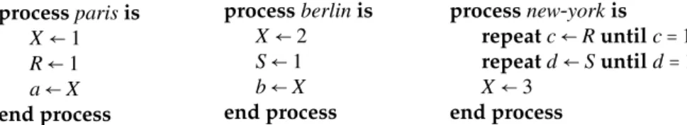
Example To illustrate the semantic ofG, we extend the original scenario that Ahamad, Niger et al use to motivate causal consistency in [ANB+95]. Consider the three processes of Figure 1, paris,
berlin, and new-york. Processes paris and berlin interact closely with one another and behave sym-metrically : they concurrently write the shared variable X, then set the flags R and S respectively to 1, and finally read X. By contrast, process new-york behaves sequentially w.r.t. paris and berlin: new-york waits for paris and berlin to write on X, using the flags R and S, and then writes X.
process paris is X← 1 R← 1 a← X end process process berlin is X← 2 S← 1 b← X end process
process new-york is repeat c← R until c = 1 repeat d← S until d = 1 X← 3
end process
Figure 1: new-york does not need to be closely synchronized with paris and berlin, calling for a hybrid form of consistency
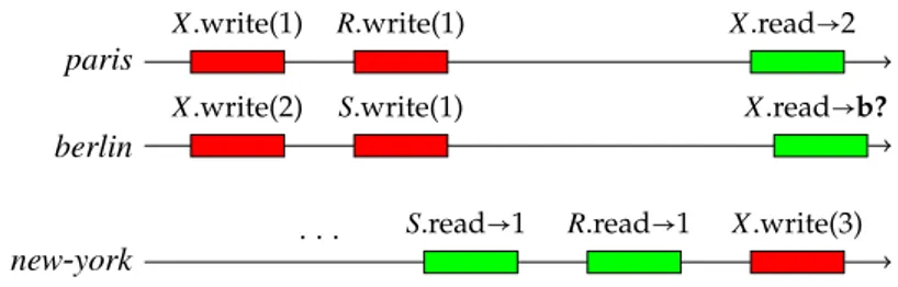
If we assume a model that provides causal consistency at a minimum, the write of X by new-york is guaranteed to be seen after the writes of paris and berlin by all processes (because new-york waits on R and S to be set to 1). Causal consistency however does not impose any consistent order on the writes of paris and berlin on X. In the execution shown on Figure 2, this means that although parisreads 2 in X (and thus sees the write of berlin after its own write), berlin might still read 1 in b(thus perceiving ‘X.write(1)’ and ‘X.write(2)’ in the opposite order to that of paris).
Sequential consistency removes this ambiguity: in this case, in Figure 2, berlin can only read 2 (the value it wrote) or 3 (written by new-york), but not 1. Sequential consistency is however too
paris
X.write(1) R.write(1) X.read→2
berlin
X.write(2) S.write(1) X.read→b?
new-york . . .
S.read→1 R.read→1 X.write(3)
Figure 2: Executing the program of Figure 1.
p b
ny
Figure 3: Capturing the synchronization needs of Fig. 1 with a proximity graphG
strong here: because the write operation of new-york is already causally ordered with those of parisand berlin, this operation does not need any additional synchronization effort. This situation can be seen as an extension of the write concurrency freedom condition introduced in [ANB+95]:
new-york is here free of concurrent write w.r.t. paris and berlin, making causal consistency equiv-alent to sequential consistency for new-york. paris and berlin however write to X concurrently, in which case causal consistency is not enough to ensure strongly consistent results.
If we assume paris and berlin execute in the same data center, while new-york is located on a distant site, this example illustrates a more general case in which, because of a program’s logic or activity patterns, no operations at one site ever conflict with those at another. In such a situation, rather than enforce a strong (and costly) consistency in the whole system, we propose a form of consistency that is strong for processes within the same site (here paris and berlin), but weak between sites (here between paris,berlin on one hand and new-york on the other).
In our model, the synchronization needs of individual processes are captured by the proxim-ity graph G introduced at the start of this section and shown in Figure 3: paris and berlin are connected, meaning the operations they execute should be perceived as strongly consistent w.r.t. one another ; new-york is neither connected to paris nor berlin, meaning a weaker consistency is allowed between the operations executed at new-york and those of paris and berlin.
2.2.2
Fisheye consistency for the pair (sequential consistency, causal
consis-tency)
When applied to the scenario of Figure 2, fisheye consistency combines two consistency condi-tions (a strong and a weaker one, here causal and sequential consistency) and a proximity graph to form an hybrid distance-based consistency condition, which we callG-fisheye (SC,CC)-consistency. The intuition in combining SC and CC is to require that (write) operations be observed in the same order by all processes if:
• They are causally related (as in causal consistency), • Or they occur on “close” nodes (as defined byG).
Formal definition Formally, we say that a history ̂HisG-fisheye (SC,CC)-consistent if: • There is a causal order↝Hinduced by ̂H(as in causal consistency); and
p
op1p: X.write(2) op2p: Y .write(4)
q
op1q: X.write(3) op2q: Y .read→4 op3q: Y .read→5
r
op1r: X.read→2 op2r: X.read→3 op3r: Y .write(5)
s
op1s: X.read→3 op2s: X.read→x? op3s: Y .read→5 op4s: Y .read→y?
q p
r s
Figure 4: IllustratingG-fisheye (SC,CC)-consistency • ↝Hcan be extended to a subsuming order
★ ↝H,G(i.e.↝H⊆ ★ ↝H,G) so that ∀p,q ∈ G ∶ (★ ↝H,G)∣{p,q} is a total order
where(↝★H,G)∣({p,q}∩W) is the restriction of ★
↝H,Gto the write operations of p and q; and
• for each process pithere is a history ̂Sithat
– (a) is sequential and legal;
– (b) is equivalent to ̂H∣(pi+W); and
– (c) respects↝★H,G, i.e.,( ★
↝H,G)∣(pi+W) ⊆ (→Si).
If we apply this definition to the example of Figure 2 with the proximity graph proposed in Figure 3 we obtain the following: because paris and berlin are connected inG, X.write(1) by paris and X.write(2) by berlin must be totally ordered in↝★H,G(and hence in any sequential history ̂Si
perceived by any process pi). X.write(3) by new-york must be ordered after the writes on X by
parisand berlin because of the causality imposed by↝H. As a result, if the system isG-fisheye
(SC,CC)-consistent, b? can be equal to 2 or 3, but not to 1. This set of possible values is as in sequential consistency, with the difference thatG-fisheye (SC,CC)-consistency does not impose any total order on the operation of new-york.
Given a system of n processes, let∅ denote the graph G with no edges, and K denote the graph G with an edge connecting each pair of distinct processes. It is easy to see that CC is ∅-fisheye (SC,CC)-consistency. Similarly SC is K-fisheye (SC,CC)-consistency.
A larger example Figure 4 and Table 1 illustrate the semantic ofG-fisheye (SC,CC) consistency on a second, larger, example. In this example, the processes p and q on one hand, and r and s on the other hand, are neighbors in the proximity graphG (shown on the left). There are two pairs of write operations: op1pand op1qon the register X, and op2pand op3r on the register Y . In a sequentially consistency history, both pairs of writes must be seen in the same order by all processes. As a consequence, if r sees the value 2 first (op1r) and then the value 3 (op2r) for X, s must do the same, and only the value 3 can be returned by x?. For the same reason, only the value 3can be returned by y?, as shown in the first line of Table 1.
In a causally consistent history, however, both pairs of writes ({op1 p,op 1 q} and {op 2 p,op 3 r}) are
causally independent. As a result, any two processes can see each pair in different orders. x? may return 2 or 3, and y? 4 or 5 (second line of Table 1).
G-fisheye (SC,CC)-consistency provides intermediate guarantees: because p and q are neigh-bors inG, op1pand op1qmust be observed in the same order by all processes. x? must return 3, as in a sequentially consistent history. However, because p and r are not connected inG, op2pand op3r
Table 1: Possible executions for the history of Figure 4
Consistency x? y?
Sequential Consistency 3 5 Causal Consistency {2,3} {4,5} G-fisheye (SC,CC)-consistency 3 {4,5}
may be seen in different orders by different processes (as in a causally consistent history), and y? may return 4 or 5 (last line of Table 1).
3
Implementing Fisheye Consistency
Our implementation ofG-fisheye (SC,CC)-consistency relies on a broadcast operation with hybrid ordering guarantees. In this section, we present this hybrid broadcast abstraction, before moving on the actual implementation of ofG-fisheye (SC,CC)-consistency in Section 3.3.
3.1
G-fisheye (SC,CC)-broadcast: definition
The hybrid broadcast we proposed, denotedG-(SC,CC)-broadcast, is parametrized by a proximity graphG which determines which kind of delivery order should be applied to which messages, according to the position of the sender in the graphG. Messages (SC,CC)-broadcast by processes which are neighbors in G must be delivered in the same order at all the processes, while the delivery of the other messages only need to respect causal order.
The (SC,CC)-broadcast abstraction provides the processes with two operations, denoted TOCO broadcast() and TOCO deliver(). We say that messages are broadcast and toco-delivered.
Causal message order. Let M be the set of messages that are toco-broadcast. The causal message delivery order, denoted↝M, is defined as follows [BJ87, RST91]. Let m1, m2∈ M; m1↝Mm2, iff one
of the following conditions holds:
• m1and m2have been toco-broadcast by the same process, with m1first;
• m1was toco-delivered by a process pibefore this process toco-broadcast m2;
• There exists a message m such that(m1↝Mm) ∧ (m ↝Mm2).
Definition of theG-fisheye (SC,CC)-broadcast. The (SC,CC)-broadcast abstraction is defined by the following properties.
• Validity. If a process toco-delivers a message m, this message was toco-broadcast by some pro-cess. (No spurious message.)
• Integrity. A message is toco-delivered at most once. (No duplication.)
•G-delivery order. For all the processes p and q such that (p,q) is an edge of G, and for all the messages mpand mqsuch that mpwas toco-broadcast by p and mqwas toco-broadcast by q,
if a process toco-delivers mpbefore mq, no process toco-delivers mqbefore mp.
• Termination. If a process toco-broadcasts a message m, this message is toco-delivered by all pro-cesses.
It is easy to see that ifG has no edges, this definition boils down to causal delivery, and if G is fully connected (clique), this definition specifies total order delivery respecting causal order. Finally, ifG is fully connected and we suppress the “causal order” property, the definition boils to total order delivery.
3.2
G-fisheye (SC,CC)-broadcast: algorithm
3.2.1
Local variables.
To implement theG-fisheye (SC,CC)-broadcast abstraction, each process pi manages three local
variables.
• causali[1..n] is a local vector clock used to ensure a causal delivery order of the messages;
causali[ j] is the sequence number of the next message that piwill toco-deliver from pj.
• totali[1..n] is a vector of logical clock values such that totali[i] is the local logical clock of pi
(Lamport’s clock), and totali[ j] is the value of totalj[ j] as known by pi.
• pendingiis a set containing the messages received and not yet toco-delivered by pi.
3.2.2
Description of the algorithm.
Let us remind that for simplicity, we assume that the channels are FIFO. Algorithm 1 describes the behavior of a process pi. This behavior is decomposed into four parts.
The first part (lines 1-6) is the code of the operation TOCO broadcast(m). Process pi first
in-creases its local clock totali[i] and sends the protocol messageTOCOBC(m,⟨causali[⋅],totali[i],i⟩) to
each other process. In addition to the application message m, this protocol message carries the control information needed to ensure the correct toco-delivery of m, namely, the local causality vector (causali[1..n]), and the value of the local clock (totali[i]). Then, this protocol message is
added to the set pendingi and causali[i] is increased by 1 (this captures the fact that the future
application messages toco-broadcast by piwill causally depend on m).
The second part (lines 7-14) is the code executed by pi when it receives a protocol message TOCOBC(m,⟨s causmj[⋅], s totmj, j⟩) from pj. When this occurs pi adds first this protocol message
to pendingi, and updates its view of the local clock of pj (totali[ j]) to the sending date of the
protocol message (namely, s totmj ). Then, if the local clock of piis late (totali[i] ≤ s totmj), picatches
up (line 11), and informs the other processes of it (line 12).
The third part (lines 15-17) is the processing of a catch up message from a process pj. In this
case, pi updates its view of pj’s local clock to the date carried by the catch up message. Let us
notice that, as channels are FIFO, a view stotali[ j] can only increase.
The final part (lines 18-31) is a background task executed by pi, where the application messages
are toco-delivered. The set C contains the protocol messages that were received, have not yet been toco-delivered, and are “minimal” with respect to the causality relation↝M. This
minimal-ity is determined from the vector clock s causm
j[1..n], and the current value of pi’s vector clock
(causali[1..n]). If only causal consistency was considered, the messages in C could be delivered.
Then, piextracts from C the messages that can be toco-delivered. Those are usually called stable
messages. The notion of stability refers here to the delivery constraint imposed by the proximity graphG. More precisely, a set T1is first computed, which contains the messages of C that (thanks
Algorithm 1TheG-fisheye (SC,CC)-broadcast algorithm executed by pi 1: operation TOCO broadcast(m)
2: totali[i] ← totali[i]+1
3: for all pj∈ Π∖{pi} do sendTOCOBC(m,⟨causali[⋅],totali[i],i⟩) to pj 4: pendingi← pendingi∪⟨m,⟨causali[⋅],totali[i],i⟩⟩
5: causali[i] ← causali[i]+1 6: end operation
7: on receivingTOCOBC(m,⟨s causmj[⋅],s totmj , j⟩)
8: pendingi← pendingi∪⟨m,⟨s causmj[⋅],s totmj, j⟩⟩
9: totali[ j] ← s totmj ▷ Last message from pjhad timestamp s totmj 10: if totali[i] ≤ s totmj then
11: totali[i] ← s totmj +1 ▷ Ensuring global logical clocks 12: for all pk∈ Π∖{pi} do sendCATCH UP(totali[i],i) to pk
13: end if
14: end on receiving
15: on receivingCATCH UP(last datej, j) 16: totali[ j] ← last datej
17: end on receiving
18: background task T is
19: loop forever
20: wait until C≠ ∅ where
21: C≡ {⟨m,⟨s causmj[⋅],s totmj, j⟩⟩ ∈ pendingi∣ s causm
j[⋅] ≤ causali[⋅]} 22: wait until T1≠ ∅ where
23: T1≡ {⟨m,⟨s causmj[⋅],s totmj, j⟩⟩ ∈ C ∣ ∀pk∈ NG(pj) ∶ ⟨totali[k],k⟩ > ⟨s tot m j, j⟩} 24: wait until T2≠ ∅ where
25: T2≡ ⎧⎪⎪⎪ ⎪⎪ ⎨⎪⎪⎪ ⎪⎪⎩⟨m,⟨s caus m j[⋅],s totmj, j⟩⟩ ∈ T1 RRRRR RRRRR RRRRR RRR ∀pk∈ NG(pj), ∀⟨mk,⟨s causmkk[⋅],s totkmk, k⟩⟩ ∈ pendingi∶ ⟨s totmk k , k⟩ > ⟨s tot m j, j⟩ ⎫⎪⎪⎪ ⎪⎪ ⎬⎪⎪⎪ ⎪⎪⎭ 26: ⟨m0,⟨s causmj0 0[⋅],s tot m0 j0 , j0⟩⟩ ← arg min ⟨m,⟨s causm j[⋅],s totmj, j⟩⟩∈T2 {⟨s totm j, j⟩} 27: pendingi← pendingi∖⟨m0,⟨s causmj00[⋅],s totmj, j0⟩⟩
28: TOCO deliver(m0) to application layer
29: if j0≠ i then causali[ j0] ← causali[ j0]+1 end if ▷ for causali[i] see line 5 30: end loop forever
to the FIFO channels and the catch up messages) cannot be made unstable (with respect to the total delivery order defined byG) by messages that piwill receive in the future. Then the set T2
is computed, which is the subset of T1such that no message received, and not yet toco-delivered,
could make incorrect – w.r.t.G – the toco-delivery of a message of T2.
Once a non-empty set T2 has been computed, pi extracts the message m whose timestamp
⟨s totm
j[ j], j⟩ is “minimal” with respect to the timestamp-based total order (pj is the sender of
m). This message is then removed from pendingiand toco-delivered. Finally, if j≠ i, causali[ j] is
increased to take into account this toco-delivery (all the messages m′toco-broadcast by p iin the
future will be such that m↝ m′, and this is encoded in causal
i[ j]). If j = i, this causality update was
done at line 5.
Theorem 1. Algorithm 1 implements aG-fisheye (SC,CC)-broadcast.
3.2.3
Proof of Theorem 1
The proof combines elements of the proofs of the traditional causal-order [BSS91, RST91] and total-order broadcast algorithms [Lam78, AW94] on which Algorithm 1 is based. It relies in par-ticular on the monoticity of the clocks causali[1..n] and totali[1..n], and the reliability and FIFO
properties of the underlying communication channels. We first prove some useful lemmata, be-fore proving termination, causal order, andG-delivery order in intermediate theorems. We finally combine these intermediate results to prove Theorem 1.
We use the usual partial order on vector clocks:
C1[⋅] ≤ C2[⋅] iff ∀pi∈ Π ∶ C1[i] ≤ C2[i]
with its accompanying strict partial order:
C1[⋅] < C2[⋅] iff C1[⋅] ≤ C2[⋅]∧C1[⋅] ≠ C2[⋅]
We use the lexicographic order on the scalar clocks⟨s totj, j⟩:
⟨s totj, j⟩ < ⟨s toti, i⟩ iff (s totj< s toti)∨(s totj= s toti∧i < j)
We start by three useful lemmata on causali[⋅] and totali[⋅]. These lemmata establish the traditional
properties expected of logical and vector clocks.
Lemma 1. The following holds on the clock values taken by causali[⋅]:
1. The successive values taken by causali[⋅] in Process piare monotonically increasing.
2. The sequence of causali[⋅] values attached to TOCOBCmessages sent out by Process piare
strictly increasing.
Proof Proposition 1 is derived from the fact that the two lines that modify causali[⋅] (lines 5,
and 29) only increase its value. Proposition 2 follows from Proposition 1 and the fact that line 5 insures successiveTOCOBCmessages cannot include identical causali[i] values. ◻Lemma1
Lemma 2. The following holds on the clock values taken by totali[⋅]:
1. The successive values taken by totali[i] in Process piare monotonically increasing.
2. The sequence of totali[i] values included inTOCOBCandCATCH UPmessages sent out by
3. The successive values taken by totali[⋅] in Process piare monotonically increasing.
Proof Proposition 1 is derived from the fact that the lines that modify totali[i] (lines 2 and 11) only
increase its value (in the case of line 11 because of the condition at line 10). Proposition 2 follows from Proposition 1, and the fact that lines 2 and 11 insures successiveTOBOBCand CATCH UP
messages cannot include identical totali[i] values.
To prove Proposition 3, we first show that:
∀ j ≠ i ∶ the successive values taken by totali[ j] in piare monotonically increasing. (1)
For j≠ i, totali[ j] can only be modified at lines 9 and 16, by values included in TOBOBCand CATCH UP messages, when these messages are received. Because the underlying channels are FIFO and reliable, Proposition 2 implies that the sequence of last datejand s totmj values received
by pifrom pjis also strictly increasing, which shows equation (1).
From equation (1) and Proposition 1, we conclude that the successive values taken by the vector totali[⋅] in piare monotonically increasing (Proposition 3). ◻Lemma2
Lemma 3. Consider an execution of the protocol. The following invariant holds: for i≠ j, if m is a message sent from pjto pi, then at any point of pi’s execution outside of lines 28-29, s causmj[ j] <
causali[ j] iff that m has been toco-delivered by pi.
Proof We first show that if m has been toco-delivered by pi, then s causmj[ j] < causali[ j], outside
of lines 28-29. This implication follows from the condition s causm
j[⋅] ≤ causali[⋅] at line 21, and the
increment at line 29.
We prove the reverse implication by induction on the protocol’s execution by process pi. When
piis initialized causali[⋅] is null:
causali0[⋅] = [0⋯0] (2)
because the above is true of any process, with Lemma 2, we also have
s causmj[⋅] ≥ [0⋯0] (3)
for all message m that is toco-broadcast by Process pj.
(2) and (3) imply that there are no messages sent by pj so that s causmj[ j] < causali0[ j], and the
Lemma is thus true when pistarts.
Let us now assume that the invariant holds at some point of the execution of pi. The only step
at which the invariant might become violated in when causali[ j0] is modified for j0≠ i at line 29.
When this increment occurs, the condition s causmj0[ j0] < causali[ j0] of the lemma potentially
be-comes true for additional messages. We want to show that there is only one single additional message, and that this message is m0, the message that has just been delivered at line 28, thus
completing the induction, and proving the lemma. For clarity’s sake, let us denote causal○
i[ j0] the value of causali[ j0] just before line 29, and
causal●
i[ j0] the value just after. We have causali●[ j0] = causal○i[ j0]+1.
We show that s causm0
j0[ jo] = causal
○
i[ j0], where s causmj00[⋅] is the causal timestamp of the message
m0delivered at line 28. Because m0is selected at line 26, this implies that m0∈ T2⊆ T1⊆ C. Because
m0∈ C, we have
s causm0
j0[⋅] ≤ causal
○
i[⋅] (4)
at line 21, and hence
s causm0
j0[ j0] ≤ causal
○
At line 21, m0 has not been yet delivered (otherwise it would not be in pendingi). Using the
contrapositive of our induction hypothesis, we have s causm0 j0[ j0] ≥ causal ○ i[ j0] (6) (5) and (6) yield s causm0 j0[ j0] = causal ○ i[ j0] (7)
Because of line 5, m0is the only message tobo broadcast by Pj0whose causal timestamp verifies
(7). From this unicity and (7), we conclude that after causali[ j0] has been incremented at line 29,
if a message m sent by Pj0 verifies s caus
m
j0[ j0] < causal
●
i[ j0], then
• either s causmj0[ j0] < causal
●
i[ j0]−1 = causal○i[ j0], and by induction assumption, m has already
been delivered; • or s causm
j0[ j0] = causal
●
i[ j0] − 1 < causali○[ j0], and m = m0, and m has just been delivered at
line 28.
◻Lemma3
Termination
Theorem 2. All messages toco-broadcast using Algorithm 1 are eventually toco-delivered by all processes in the system.
Proof We show Termination by contradiction. Assume a process pitoco-broadcasts a message mi
with timestamp⟨s causmi
i [⋅],s tot mi
i , i⟩, and that miis never toco-delivered by pj.
If i≠ j, because the underlying communication channels are reliable, pjreceives at some point
theTOCOBCmessage containing mi(line 7), after which we have
⟨mi,⟨s causmii[⋅],s totimi, i⟩⟩ ∈ pendingj (8)
If i= j, miis inserted into pendingiimmediately after being toco-broadcast (line 4), and (8) also
holds.
mimight never be toco-delivered by pjbecause it never meets the condition to be selected into
the set C of pj (noted Cj below) at line 21. We show by contradiction that this is not the case.
First, and without loss of generality, we can choose miso that it has a minimal causal timestamp
s causmi
i [⋅] among all the messages that j never toco-delivers (be it from pi or from any other
process). Minimality means here that
∀mx, pjnever delivers mx⇒ ¬(s causmxx< s caus mi
i ) (9)
Let us now assume miis never selected into Cj, i.e., we always have
¬(s causmi
i [⋅] ≤ causalj[⋅]) (10)
This means there is a process pkso that
s causmi
If i= k, we can consider the message m′
i sent by i just before mi (which exists since the above
implies s causmi
i [i] > 0). We have s caus m′i
i [i] = s caus mi
i [i]−1, and hence from (11) we have
s causm
′ i
i [i] ≥ causalj[k] (12)
Applying Lemma 3 to (12) implies that pj never toco-delivers m′i either, with s caus m′i i [i] <
s causmi
i [i] (by way of Proposition 2 of Lemma 1), which contradicts (9).
If i≠ k, applying Lemma 3 to causali[⋅] when pitoco-broadcasts miat line 3, we find a message mk
sent by pkwith s causmkk[k] = s causimi[k]−1 such that mkwas received by pibefore pitoco-broadcast
mi. In other words, mkbelongs to the causal past of mi, and because of the condition on C (line 21)
and the increment at line 29, we have s causmk
k [⋅] < s caus mi
i [⋅] (13)
As for the case i= k, (11) also implies
s causmk
k [k] ≥ causalj[k] (14)
which with Lemma 3 implies that that pj never delivers the message mk from pk, and with (13)
contradicts mi’s minimality (9).
We conclude that if a message mi from pi is never toco-delivered by pj, after some point mi
remains indefinitely in Cj
mi∈ Cj (15)
Without loss of generality, we can now choose mi with the smallest total order timestamp
⟨s totmi
i , i⟩ among all the messages never delivered by pj. Since these timestamps are totally
or-dered, and no timestamp is allocated twice, there is only one unique such message.
We first note that because channels are reliable, all processes pk∈ NG(pi) eventually receive the TOCOBCprotocol message of pithat contains mi(line 7 and following). Lines 10-11 together with
the monotonicity of totalk[k] (Proposition 1 of Lemma 2), insure that at some point all processes
pkhave a timestamp totalk[k] strictly larger than s totimi:
∀pk∈ NG(pi) ∶ totalk[k] > s tot mi
i (16)
Since all changes to totalk[k] are systematically rebroadcast to the rest of the system usingTO -COBCorCATCHUPprotocol messages (lines 2 and 11), pj will eventually update totalj[k] with a
value strictly higher than s totmi
i . This update, together with the monotonicity of totalj[⋅]
(Propo-sition 3 of Lemma 2), implies that after some point:
∀pk∈ NG(pi) ∶ totalj[k] > s tot mi
i (17)
and that miis selected in T1j. We now show by contradiction that mieventually progresses to T2j.
Let us assume minever meets T2j’s condition. This means that every time T2jis evaluated we have:
∃pk∈ NG(pi),∃⟨mk,⟨s caus mk k [⋅],s tot mk k , k⟩⟩ ∈ pendingj∶ ⟨s totmk k , k⟩ ≤ ⟨s tot m i , i⟩ (18)
Note that there could be different pkand mk satisfying (18) in each loop of Task T . However,
because NG(pi) is finite, the number of timestamps ⟨s totkmk, k⟩ such that ⟨s totkmk, k⟩ ≤ ⟨s totim, i⟩ is
also finite. There is therefore one process pk0 and one message mk0 that appear infinitely often in
the sequence of(pk, mk) that satisfy (18). Since mk0 can only be inserted once into pendingj, this
means mk0 remains indefinitely into T
j
2, and hence pendingj, and is never delivered. (18) and the
fact that i≠ k0(because pi/∈ NG(pi)) yields
⟨s totmk0
k , k0⟩ < ⟨s tot m
i , i⟩ (19)
which contradicts our assumption that mi has the smallest total order timestamps ⟨s totimi, i⟩
among all messages never delivered to pj. We conclude that after some point mi remains
in-definitely into T2j.
mi∈ T2j (20)
If we now assume miis never returned by argmin at line 26, we can repeat a similar argument
on the finite number of timestamps smaller than⟨s totm
i , i⟩, and the fact that once they have been
removed form pendingj (line 27), messages are never inserted back, and find another message
mk with a strictly smaller time-stamp that pj that is never delivered. The existence of mk
con-tradicts again our assumption on the minimality of mi’s timestamp⟨s totim, i⟩ among undelivered
messages.
This shows that miis eventually delivered, and ends our proof by contradiction. ◻T heorem2
Causal Order We prove the causal order property by induction on the causal order relation↝M.
Lemma 4. Consider m1 and m2, two messages toco-broadcast by Process pi, with m1
toco-broadcast before m2. If a process pjtoco-delivers m2, then it must have toco-delivered m1before
m2.
Proof We first consider the order in which the messages were inserted into pendingj(along with
their causal timestamps s causmi1∣2). For i= j, m1was inserted before m2at line 4 by assumption.
For i≠ j, we note that if pj delivers m2at line 28, then m2was received from piat line 7 at some
earlier point. Because channels are FIFO, this also means
m1was received and added to pendingjbefore m2was. (21)
We now want to show that when m2is delivered by pj, m1is no longer in pendingj, which will
show that m1has been delivered before m2. We use an argument by contradiction. Let us assume
that
⟨m1,⟨s causmi1, s tot m1
i , i⟩⟩ ∈ pendingj (22)
at the start of the iteration of Task T which delivers m2to pj. From Proposition 2 of Lemma 1, we
have
s causm1
i < s caus m2
i (23)
which implies that m1is selected into C along with m2(line 21):
⟨m1,⟨s causmi1, s totim1, i⟩⟩ ∈ C
Similarly, from Proposition 2 of Lemma 2 we have: s totm1
i < s tot m2
which implies that m1 must also belong to T1and T2(lines 23 and 25). (24) further implies that
⟨s totm2
i , i⟩ is not the minimal s tot timestamp of T2, and therefore m0≠ m2in this iteration of Task
T. This contradicts our assumption that m2was delivered in this iteration; shows that (22) must
be false; and therefore with (21) that m1was delivered before m2. ◻Lemma4
Lemma 5. Consider m1 and m2 so that m1 was toco-delivered by a process pi before pi
toco-broadcasts m2. If a process pjtoco-delivers m2, then it must have toco-delivered m1before m2.
Proof Let us note pk the process that has toco-broadcast m1. Because m2is toco-broadcasts by
pi after pi toco-delivers m1 and increments causali[k] at line 29, we have, using Lemma 3 and
Proposition 1 of Lemma 1:
s causm1
k [k] < s caus m2
i [k] (25)
Because of the condition on set C at line 21, when pjtoco-delivers m2at line 28, we further have
s causm2
i [⋅] ≤ causalj[⋅] (26)
and hence using (25)
s causm1
k [k] < s caus m2
i [k] ≤ causalj[k] (27)
Applying Lemma 3 to (27), we conclude that pjmust have toco-delivered m1when it delivers
m2. ◻Lemma5
Theorem 3. Algorithm 1 respects causal order.
Proof We finish the proof by induction on↝M. Let’s consider three messages m1, m2, m3such that
m1↝Mm3↝Mm2 (28)
and such that:
• if a process toco-delivers m3, it must have toco-delivered m1;
• if a process toco-delivers m2, it must have toco-delivered m3;
We want to show that if a process toco-delivers m2, it must have tolo-delivered m1. This follows
from the transitivity of temporal order. This result together with Lemmas 4 and 5 concludes the
proof. ◻T heorem3
G-delivery order
Theorem 4. Algorithm 1 respectsG-delivery order.
Proof Let’s consider four processes pl, ph, pi, and pj. pland phare connected inG. pl has
toco-broadcast a message ml, and phhas toco-broadcast a message mh. pihas toco-delivered mlbefore
mh. pjhas toco-delivered mh. We want to show that pjhas toco-delivered mlbefore mh.
We first show that:
⟨s totmh
h , h⟩ > ⟨s tot ml
l , l⟩ (29)
We do so by considering the iteration of the background task T (lines 18-18) of pithat toco-delivers
ml. Because ph∈ NG(pl), we have
at line 23.
If mhhas not been received by piyet, then because of Lemma 3.2, and because communication
channels are FIFO and reliable, we have: ⟨s totmh
h , l⟩ > ⟨totali[h],h⟩ (31)
which with (30) yields (29).
If mhhas already been received by pi, by assumption it has not been toco-delivered yet, and is
therefore in pendingi. More precisely we have:
⟨mh,⟨s causmhh[⋅],s tothmh, h⟩⟩ ∈ pendingi (32)
which, with ph∈ NG(pl), and the fact that ml is selected in T2iat line 25 also gives us (29).
We now want to show that pj must have toco-delivered ml before mh. The reasoning is
some-what the symmetric of some-what we have done. We consider the iteration of the background task T of pjthat toco-delivers mh. By the same reasoning as above we have
⟨totalj[l],l⟩ > ⟨s tothmh, h⟩ (33)
at line 23.
Because of Lemma 3.2, and because communication channels are FIFO and reliable, (33) and (29) imply that ml has already been received by pj. Because mhis selected in T2j at line 25, (29)
implies that mhis no longer in pendingj, and so must have been toco-delivered by pjearlier, which
concludes the proof. ◻T heorem4
Theorem 1. Algorithm 1 implements aG-fisheye (SC,CC)-broadcast. Proof
• Validity and Integrity follow from the integrity and validity of the underlying communica-tion channels, and from how a message mjis only inserted once into pendingi(at line 4 if i= j,
at line 8 otherwise) and always removed from pendingiat line 27 before it is toco-delivered
by piat line 28;
• G-delivery order follows from Theorem 4; • Causal order follows from Theorem 3; • Termination follows from Theorem 2.
◻T heorem1
3.3
An Algorithm Implementing
G-Fisheye (SC,CC)-Consistency
3.3.1
The high level object operations read and write
Algorithm 2 uses theG-fisheye (SC,CC)-broadcast we have just presented to realized G-fisheye (SC,CC)-consistency using a fast-read strategy. This algorithm is derived from the fast-read algo-rithm for sequential consistency proposed by Attiya and Welch [AW94], in which the total order broadcast has been replaced by ourG-fisheye (SC,CC)-broadcast.
The write(X,v) operation uses the G-fisheye (SC,CC)-broadcast to propagate the new value of the variable X. To insure any other write operations that must be seen before write(X,v) by piare
Algorithm 2ImplementingG-fisheye (SC,CC)-consistency, executed by pi 1: operation X.write(v)
2: TOCO broadcast(WRITE(X,v,i)) 3: deliveredi← f alse ;
4: wait until deliveredi= true 5: end operation
6: operation X.read()
7: return vx 8: end operation
9: on toco deliverWRITE(X,v, j) 10: vx← v ;
11: if(i = j) then deliveredi← true endif 12: end on toco deliver
properly processed, pienters a waiting loop (line 4), which ends after the messageWRITE(X,v,i)
that has been toco-broadcast at line 2 is toco-delivered at line 11.
The read(X) operation simply returns the local copy vxof X. These local copies are updated in
the background whenWRITE(X,v, j) messages are toco-delivered.
Theorem 5. Algorithm 2 implementsG-fisheye (SC,CC)-consistency.
3.3.2
Proof of Theorem 5
The proof uses the causal order on messages↝M provided by the G-fisheye (SC,CC)-broadcast
to construct the causal order on operations↝H. It then gradually extends↝Hto obtain ★
↝H,G. It
first uses the property of the broadcast algorithm on messages to-broadcast by processes that are neighbors inG, and then adapts the technique used in [MZR95, Ray13] to show that WW (write-write) histories are sequentially consistent. The individual histories ̂Si are obtained by taking a
topological sort of(↝★H,G)∣(pi+W).
For readability, we denote in the following rp(X,v) the read operation invoked by process p on
object X that returns a value v (X.read→ v), and wp(X,v) the write operation of value v on object
Xinvoked by process p (X.write(v)). We may omit the name of the process when not needed. Let us consider a history ̂H= (H,→poH) that captures an execution of Algorithm 2, i.e.,
po
→H
cap-tures the sequence of operations in each process (process order, po for short). We construct the causal order↝Hrequired by the definition of Section 2.2.2 in the following, classical, manner:
• We connect each read operation rp(X,v) = X.read → v invoked by process p (with v ≠ ,
the initial value) to the write operation w(X,v) = X.write(v) that generated theWRITE(X,v)
message carrying the value v to p (line 10 in Algorithm 2). In other words, we add an edge⟨w(X,v)→ rrf p(X,v)⟩ to
po
→H (with w and rpas described above) for each read operation
rp(X,v) ∈ H that does not return the initial value . We connect initial read operations r(X,)
to an element that we add to H.
We call these additional relations read-from links (noted→).rf • We take↝Hto be the transitive closure of the resulting relation.
↝H is acyclic, as assuming otherwise would imply at least one of the WRITE(X,v) messages
order, i.e., that the result of each read operation r(X,v) is the value of the latest write w(X,v) that occurred before r(X,v) in ↝H(said differently, that no read returns an overwritten value).
Lemma 6. ↝H is a causal order.
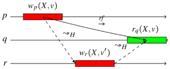
Proof We show this by contradiction. We assume without loss of generality that all values writ-ten are distinct. Let us consider wp(X,v) and rq(X,v) so that wp(X,v)
rf
→ rq(X,v), which implies
wp(X,v) ↝Hrq(X,v). Let us assume there exists a second write operation wr(X,v′) ≠ wp(X,v) on
the same object, so that
wp(X,v) ↝Hwr(X,v′) ↝Hrq(X,v) (34)
(illustrated in Figure 5). wp(X,v) ↝Hwr(X,v′) means we can find a sequence of operations opi∈ H
so that wp(X,v) →0op0...→iopi→i+1...→kwr(X,v′) (35) with→i∈ { po →H, rf
→},∀i ∈ [1,k]. The semantics ofpo→H and rf
→ means we can construct a sequence of causally related (SC,CC)-broadcast messages mi∈ M between the messages that are toco-broadcast
by the operations wp(X,v) and wr(X,v′), which we noteWRITE p(X,v) andWRITEr(X,v′)
respec-tively:
WRITE p(X,v) = m0↝Mm1...↝Mmi↝M...↝Mmk′=WRITEr(X,v′) (36)
where↝Mis the message causal order introduced in Section 3.1. We conclude thatWRITE p(X,v) ↝M WRITEr(X,v′), i.e., that
WRITE p(X,v) belongs to the causal past ofWRITEr(X,v′), and hence that q
in Figure 5 toco-deliversWRITEr(X,v′) after
WRITE p(X,v). p wp(X,v) q rq(X,v) r wr(X,v′) rf → ↝H ↝H
Figure 5: Proving that↝His causal by contradiction
We now want to show thatWRITEr(X,v′) is toco-delivered by q before q executes r
q(X,v). We
can apply the same reasoning as above to wr(X,v′) ↝Hrq(X,v), yielding another sequence of
op-erations op′ i∈ H: wr(X,v′) →′0op ′ 0...→ ′ iop ′ i→ ′ i+1...→ ′ k′′rq(X,v) (37) with→′ i∈ { po →H, rf
→}. Because rq(X,v) does not generate any (SC,CC)-broadcast message, we need to
distinguish the case where all op′
i relations correspond to the process order po
→H(i.e., op′i= po
→H,∀i).
In this case, r= q, and the blocking behavior of X.write() (line 4 of Algorithm 2), insures that
WRITEr(X,v′) is toco-delivered by q before executing r
q(X,v). If at least one op′i corresponds to
the read-from relation, we can consider the latest one in the sequence, which will denote the toco-delivery of aWRITEz(Y,w) message by q, withWRITEr(X,v′) ↝
M WRITEz(Y,w). From the causality
of the (SC,CC)-broadcast, we also conclude thatWRITEr(X,v′) is toco-delivered by q before
exe-cuting rq(X,v).
Because q toco-deliversWRITE p(X,v) beforeWRITEr(X,v′), and toco-deliversWRITEr(X,v′)
be-fore it executes rq(X,v), we conclude that the value v of vxis overwritten by v′at line 10 of
Algo-rithm 2, and that rq(X,v) does not return v, contradicting our assumption that wp(X,v) rf
→ rq(X,v),
To construct↝★H,G, as required by the definition of (SC,CC)-consistency (Section 2.2.2), we need
to order the write operations of neighboring processes in the proximity graphG. We do so as follows:
• We add an edge wp(X,v) ww
→ wq(Y,w) to ↝H for each pair of write operations wp(X,v) and
wq(Y,w) in H such that:
– (p,q) ∈ EG(i.e., p and q are connected inG);
– wp(X,v) and wq(Y,w) are not ordered in ↝H;
– The broadcast message WRITE p(X,v) of wp(X,v) has been toco-delivered before the
broadcast messageWRITE p(Y,w) of wq(Y,w) by all processes.
We call these additional edges ww links (notedww→).
• We take↝★H,Gto be the recursive closure of the relation we obtain. ★
↝H,Gis acyclic, as assuming otherwise would imply that the underlying (SC,CC)-broadcast
vio-lates causality. Because of theG-delivery order and termination of the toco-broadcast (Section 3.1), we know all pairs ofWRITE p(X,v) andWRITE p(Y,w) messages with (p,q) ∈ EG as defined above
are toco-delivered in the same order by all processes. This insures that all write operations of neighboring processes inG are ordered in↝★H,G.
We need to show that↝★H,G remains a causal order, i.e., that no read in ★
↝H,Greturns an
over-written value.
Lemma 7. ↝★H,Gis a causal order.
Proof We extend the original causal order↝Mon the messages of an (SC,CC)-broadcast execution
with the following order↝G M:
m1↝GMm2if
• m1↝Mm2; or
• m1was sent by p, m2by q,(p,q) ∈ EG, and m1is toco-delivered before m2by all processes; or
• there exists a message m3so that m1↝GMm3and m3↝GMm2.
↝G
M captures the order imposed by an execution of an (SC,CC)-broadcast on its messages. The
proof is then identical to that of Lemma 6, except that we use the order↝G
M, instead of↝M.◻Lemma7
Theorem 5. Algorithm 2 implementsG-fisheye (SC,CC)-consistency.
Proof The order↝★H,Gwe have just constructed fulfills the conditions required by the definition
ofG-fisheye (SC,CC)-consistency (Section 2.2.2): • by construction↝★H,Gsubsumes↝H(↝H⊆ ★
↝H,G);
• also by construction↝★H,G, any pair of write operations invoked by processes p,q that are
neighbors inG are ordered in↝★H,G; i.e.,( ★
To finish the proof, we choose, for each process pi, ̂Si as one of the topological sorts of
(★
↝H,G)∣(pi+W), following the approach of [MZR95, Ray13]. ̂Siis sequential by construction.
Be-cause↝★H,Gis causal, ̂Siis legal. Because ★ ↝H,Grespects po →H, ̂Siis equivalent to ̂H∣(pi+W). Finally, ̂Sirespects( ★ ↝H,G)∣(pi+W) by construction. ◻T heorem5
4
Towards Update Consistency
We now introduce the second contribution of this deliverable. This contribution follows the long quest of the (a) strongest consistency criterion (there may exist several incomparable criteria) im-plementable for different types of objects in an asynchronous system where all but one process may crash (wait-free systems [Her91]). A contribution of this line of work consists in proving that weak consistency criteria such as eventual consistency and causal consistency cannot be combined is such systems. In this second part of our work we therefore explore the enforce-ment of eventual consistency. The relevance of eventual consistency has been illustrated many times. It is used in practice in many large scale applications such as Amazon’s Dynamo highly available key-value store [DHJ+07]. It has been widely studied and many algorithms have been
proposed to implement eventually consistent shared object. Conflict-free replicated data types (CRDT) [SPBZ11] give sufficient conditions on the specification of objects so that they can be im-plemented. More specifically, if all the updates made on the object commute or if the reachable states of the object form a semi-lattice then the object has an eventually consistent implementation [SPBZ11]. Unfortunately, many useful objects are not CRDTs.
The limitations of eventual consistency led to the study of stronger criteria such as strong even-tual consistency [SPB+11]. Indeed, eventual consistency requires the convergence towards a
com-mon state without specifying which states are legal. In order to prove the correctness of a program, it is necessary to fully specify which behaviors are accepted for an object. The meaning of an op-eration often depends on the context in which it is executed. The notion of intention is widely used to specify collaborative editing [SJZ+98, LZM00]. The intention of an operation not only
depends on the operation and the state on which it is done, but also on the intentions of the con-current operations. In another solution [BZP+12], it is claimed that, it is sufficient to specify what
the concurrent execution of all pairs of non-commutative operations should give (e.g. an error state). This result, acceptable for the shared s et, cannot be extended to other more complicated objects. In this case, any partial order of updates can lead to a different result. This approach was formalized in [BGYZ14], where the concurrent specification of an object is defined as a function of partially ordered sets of updates to a consistent state leading to specifications as complicated as the implementations themselves. Moreover, a concurrent specification of an object uses the notion of concurrent events. In message-passing systems, two events are concurrent if they are produced by different processes and each process produced its event before it received the notifi-cation message from the other process. In other words, the notion of concurrency depends on the implementation of an object not on its specification. Consequently, the final user may not know if two events are concurrent without explicitly tracking the underlying messages. A specification should be independent of the system on which it is implemented.
To avoid restricting our results to a given data structure, we first define a class of data types called UQ-ADT for update-query abstract data type. This class encompasses all data structures where an operation either modifies the state of the object (update) or returns a function on the current state of the object (query). This class excludes data types such as a stack where the pop op-eration removes the top of the stack and returns it (update and query at the same time). However, such operations can always be separated into a query and an update (lookup top and delete top in the case of the stack) which is not a problem as, in weak consistency models, it is impossible to ensure atomicity anyway. Based on this notion, we then present three main contributions.
• We prove that in a wait-free asynchronous system, it is not possible to implement eventual and causal consistency for all UQ-ADTs.
• We introduce update consistency, a new consistency criterion stronger than eventual con-sistency and for which the converging state must be consistent with a linearization of the updates.
• Finally, we prove that for any UQ-ADT object with a sequential specification there exists an update consistent implementation by providing a generic construction.
4.1
Abstract Data Types and Consistency Criteria
Before introducing the new consistency criterion, this section formalizes the notion of object and how a consistency criterion is defined. In distributed systems, sharing objects is a way to ab-stract message-passing communication between processes. The abab-stract type of these objects has a sequential specification, which we describe by means of a transition system that characterizes the sequential histories allowed for this object. However, shared objects are implemented in a distributed system using replication and the events of the distributed history generated by the execution of a distributed program is a partial order [Lam78]. The consistency criterion makes the link between the sequential specification of an object and a distributed execution that invokes it. This is done by characterizing the partially ordered histories of the distributed program that are acceptable. The formalization used in this deliverable is explained with more details in [PPJM14]. An abstract data type is specified using a transition system very close to Mealy machines [Mea55] except that infinite transition systems are allowed as many objects have an unbounded specification. As stated above, this part of our work focuses on ”update-query” objects. On the one hand, the updates have a side-effect that usually affects the state of the object (hence all pro-cesses), but return no value. They correspond to transitions between abstract states in the tran-sition system. On the other hand, the queries are read-only operations. They produce an output that depends on the state of the object. Consequently, the input alphabet of the transition system is separated into two classes of operations (updates and queries).
Definition 1(Update-query abstract data type). An update-query abstract data type (UQ-ADT) is a tuple O= (U,Qi, Qo, S, s0, T, G) such that:
• U is a countable set of update operations;
• Qiand Qoare countable sets called input and output alphabets; Q= Qi×Qois the set of query
operations. A query operation(qi, qo) ∈ Q is denoted qi/qo(query qireturns value qo).
• S is a countable set of states; • s0∈ S is the initial state;
• T∶ S×U → S is the transition function; • G∶ S×Qi→ Qois the output function.
A sequential history is a sequence of operations. An infinite sequence of operations (wi)i∈N∈
(U ∪ Q)ωis recognized by O if there exists an infinite sequence of states(s
i)i≥1∈ Sω(note that s0
is the initial state) such that for all i∈ N, T(si, wi) = si+1 if wi∈ U or si= si+1 and G(si, qi) = qo if
wi= qi/qo∈ Q. The set of all infinite sequences recognized by O and their finite prefixes is denoted
by L(O). Said differently, L(O) is the set of all the sequential histories allowed for O.
In the following, we use replicated sets as the key example. Three kinds of operations are possible: two update operation by element, namely insertion (I) and deletion (D) and a query operation read (R) that returns the values that belong to the set. Let Val be the support of the
replicated set (it contains the values that can be inserted/deleted). At the beginning, the set is empty and when an element is inserted, it becomes present until it is deleted. More formally, it corresponds to the UQ-ADT given in Example 1.
Example 1(Specification of the set). Let Val be a countable set, called support. The set objectSVal
is the UQ-ADT(U,Qi, Qo, S,∅,T,G) with:
• U= {I(v),D(v) ∶ v ∈ Val};
• Qi= {R}, and Qo= S = P<∞(Val) contain all the finite subsets of Val;
• for all s∈ S and v ∈ Val, G(s,R) = s,
T(s,I(v)) = s∪{v} and T(s,D(v)) = s∖{v}.
The set U of updates is the set of all insertions and deletions of any value of Val. The set of queries Qicontains a unique operation R, a read operation with no parameter. A read operation
may return any value in Qo, the set of all finite subsets of Val. The set S of the possible states is
the same as the set of possible returned values Qoas the read query returns the content of the set
object. I(v) (resp. D(v)) with v ∈ Val denotes an insertion (resp. a deletion) operation of the value vinto the set object. R/s denotes a read operation that returns the set s representing the content of the set.
During an execution, the participants invoke an object instance of an abstract data type using the associated operations (queries and updates). This execution produces a set of partially ordered events labelled by the operations of the abstract data type. This representation of a distributed history is generic enough to model a large number of distributed systems. For example, in the case of communicating sequential processes, an event a precedes an event b in the program order if they are executed by the same process in that sequential order. It is also possible to model more complex modern systems in which new threads are created and destroyed dynamically, or peer-to-peer systems where peers may join and leave.
Definition 2(Distributed History). A distributed history is a tuple H= (U,Q,E,Λ,↦):
• U and Q are disjoint countable sets of update and query operations, and all queries q∈ Q are in the form q= qi/qo;
• E is a countable set of events; • Λ∶ E → U ∪Q is a labelling function;
• ↦⊂ E ×E is a partial order called program order, such that for all e ∈ E, {e′∈ E ∶ e′↦ e} is finite.
Let H= (U,Q,E,Λ,↦) be a history. The sets UH= {e ∈ E ∶ Λ(e) ∈ U} and QH= {e ∈ E ∶ Λ(e) ∈ Q}
de-note its sets of update and query events respectively. We also define some projections on the his-tories. The first one allows to withdraw some events: for F⊂ E, HF= (U,Q,F,Λ∣F,↦ ∩(F ×F)) is the
history that contains only the events of F. The second one allows to substitute the order relation: if → is a partial order that respects the definition of a program order (↦), H→= (U,Q,E,Λ,→ ∩(E ×E))
is the history in which the events are ordered by→. Note that the projections commute, which allows the notation H→
F.
Definition 3(Linearizations). Let H= (U,Q,E,Λ,↦) be a distributed history. A linearization of H corresponds to a sequential history that contains the same events as H in an order consistent with the program order. More precisely, it is a word Λ(e0)...Λ(en)... such that {e0, . . . , en, . . .} = E and
for all i and j, if i< j, ej /↦ ei. We denote by lin(H) the set of all linearizations of H.
Definition 4(Consistency criterion). A consistency criterion C characterizes which histories are allowed for a given data type. It is a function C that associates with any UQ-ADT O, a set of distributed histories C(O). A shared object (instance of an UQ-ADT O) is C-consistent if all the histories it allows are in C(O).