Dark noise calibration of the Super-Kamiokande outer detector

Dark Noise Calibration of the Super-Kamiokande

Outer Detector

by

John G. Focht

Submitted to the Department of Physics

in partial fulfillment of the requirements for the degree of

Bachelor of Science in Physics

at the

MASSACHUSETTS INSTITUTE OF TECHNOLOGY

June 2004

() Massachusetts Institute of Technology 2004. All rights reserved.

Author .

//~

~Department

of Physics

May 7, 2004

Certified by ...

'I.... . . .

_{ate Scholberg}

Professor of Physics

Thesis Supervisor

Accepted

by...

Professor Dave E. Pritchard

Senior Thesis Coordinator, Department of Physics

MASSACHUSETTS INSTIiTUTE OF TECHNOLOGY

Dark Noise Calibration of the Super-Kamiokande Outer

Detector

by

John G. Focht

Submitted to the Department of Physics on May 7, 2004, in partial fulfillment of the

requirements for the degree of Bachelor of Science in Physics

Abstract

The process for calculating the single photoelectron gain in the Super-Kamiokande outer detector has been streamlined. The original technique used optic fibers to expose the detector's photomultiplier tubes to known amounts of light in order to determine the signal response to one photoelectron. This process was long and re-quired data collection to halt during calibration. The new technique makes use of the background noise hits that are recorded in the time before an event that triggers the outer detector. By assuming that these hits are single photoelectrons, the data points provide a charge calibration that is fast, does not intrude on data collection, and presents little compromise of accuracy. The dark noise calibration technique has already been used to adjust the voltage supplies to the photomultiplier tubes so that their gains are more uniform. It also makes it possible to check the long term stability of the gain calibration.

Thesis Supervisor: Kate Scholberg Title: Professor of Physics

Acknowledgments

I would like to acknowledge Kate Scholberg for her guidance and help in doing this work and writing this thesis.

Contents

1 Introduction 13

1.1 Neutrinos and Neutrino Detection ... . 13

1.2 The Super-Kamiokande Collaboration . . . 14

2 Outer Detector Electronics and Calibration 17 2.1 Laser Calibration Procedure ... . 18

2.2 Laser Calibration Calculations ... 18

2.3 Laser Calibration Results ... . 20

3 Outer Detector Dark Noise Calibration 23 3.1 Procedure . . . 23

3.2 Calculations ... 24

3.3 Calibration Results ... 25

3.4 Relative Uncertainties and Errors ... . 26

3.5 Calibration Adjustment Algorithm ... . 28

4 Stability of Calibration 31

List of Figures

1-1 A partially contained event in the Super-Kamiokande detector. A muon neutrino enters the inner detector and interacts with a neutron to produce a proton and a muon. The muon then escapes, leaving a trail of Cherenkov radiation in both the inner and outer detectors. The proton is shown in this diagram, but is often invisible to the detector as it remains bound in a nucleus or travels freely but below the threshold for Cherenkov radiation ... 16

2-1 A simple schematic of the laser fiber system. The outer detector PMTs record data as each fiber flashes at different attenuations. From [5]. . 19 2-2 The mean number of photoelectrons per observed hit against the

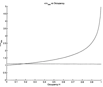
oc-cupancy. For occupancies less than 0.18, the mean for observed hits is

less than 1.1 . . . 21

2-3 A histogram showing the distribution of spe gains over the photomul-tiplier tubes in January 2003. Peaks corresponding to the old and new

PMTs are distinctly visible ... . 22

3-1 The complete data set for one PMT channel 5 during a calibration run. For the dark noise calibration, only hits between 35000 ns and 45000 ns are included in the calculations. The peak is at the actual trigger, corresponding to the flashes for the laser calibration technique ... 24

3-2 The distribution of number of tubes over dark noise gains from the laser calibration run 021373. The distribution here parallels that of the number of tubes over laser calibration gain. The bimodality between old and new tubes is still present ... 25 3-3 The graph shows the spe gain determined from the dark noise technique

against the gain calculated from the laser calibration. Each dot is one photomultiplier tube. The line is y = 0.23 + 1.05x, the best-fit line to the data ... 27 3-4 A histogram of dark noise hits for PMT channel 5 during run 023219.

The gain for this channel was measured to be 11.1 counts/pe, a fairly typical result. If all of the hits were single photoelectrons, the error would be +0.3 counts/pe. Instead, it is taken to be about ±1.1 counts/pe. 28 3-5 The beginning, middle, and end of the adjustment algorithm. The

bimodal distribution between old and new tubes because a single group. From [6] ... 29 4-1 The distribution of channels over spe gains for run 023179 on October

12, 2003. These gains are from after the adjustment algorithm. The peak at zero is from dead tubes ... 32 4-2 A histogram of spe gain drift between October 12, 2003, and November

2, 2003. The tubes are centered very tightly at zero drift ... 32 4-3 A histogram of spe gain drift between October 12, 2003, and April 29,

Chapter 1

Introduction

1.1 Neutrinos and Neutrino Detection

The neutrino is a small, almost massless particle with no charge. First postulated to exist in the 1930s to preserve conservation of energy and momentum in nuclear reactions, neutrinos were not observed until the 1950s because they rarely interact with other matter. Even today, the neutrinos remain difficult to detect.

Neutrinos exist in three types: electron neutrinos (e), muon neutrinos (v,), and tau neutrinos (v1), each related to the fundamental particle from which it takes its

name. In a charged current neutrino interaction, a neutrino interacts with a neutron to produce its corresponding particle. For example, in the interaction

ve + n p+ e- (1.1)

a neutrino interacts with a neutron using the weak force, producing a proton and an electron. Similar charged current interactions by muon or tau neutrinos would produce muons or tau particles, respectively, instead of electrons, while antineutrinos would produce the charge conjugates in each reaction, creating an antiproton and a e+, tt+, or T+. Neutrinos can also undergo neutral current interactions, which do not

produce movements of charge from particle to particle. Neutral current interactions are flavor-blind, meaning that all three types of neutrinos behave the same way.

Because neutrinos are only observable through weak interactions, neutrino de-tectors need to be large in order to provide enough interaction opportunities for a passing neutrino. The Super-Kamiokande detector, for example, uses 50,000 metric tons of water as the target for neutrino interaction. Despite the difficulty, it is still worthwhile to study neutrinos to better understand solar nuclear reactions, cosmic ray interactions with the atmosphere, and supernovas. In addition, evidence that neutrinos can oscillate among all three types has shown that neutrinos are massless.

1.2 The Super-Kamiokande Collaboration

The Super-Kamiokande Collaboration is a joint Japanese-American neutrino de-tection project located under Mount Ikenoyama in Kamioka, Japan. The Super-Kamiokande detector is a large steel cylinder filled with purified water, the neutrino interaction target. Neutrinos entering the detector interact with neutrons in the oxy-gen atoms of the water, each producing a proton and another particle which depends on the neutrino type. Antineutrinos entering the apparatus interact with protons to produce neutrons and positrons. The charged particles produced, whether electron, muon, or antiparticle, move faster than the speed of light in water, creating a cone of Cherenkov radiation, the luminal equivalent of a sonic boom. The steel cylinder orig-inally contained over 11,000 photomultiplier tubes which face into the tank to detect this light, but an accident in November 2001 destroyed many of the tubes. Subse-quent reconstruction in 2002 restored 47 percent of the inner detector PMTs.[4] By measuring the size, shape, location, and brightness of the ring where the cone meets the cylinder, one can determine the energy, direction, and type of product particle. This, in turn, allows one to determine properties of the original neutrino.

In addition, a second detector array faces outward from the cylinder, light-sealed from the first and completely reconstructed following the 2001 accident. This outer detector consists of 1,885 PMTs which are used to distinguish actual neutrino events from background noise. If an event is recorded by the inner detector and not the outer detector, it is likely a neutrino interaction inside the Super-Kamiokande detector, but

if it is recorded by both, it is simply a stray particle. Background noise at the Super-Kamiokande detector is mostly due to radioactive decay in the surrounding rock, radon within the water, and muons resulting from cosmic ray interactions in the

atmosphere. [4]

The outer detector is also useful in measurement of partially contained neutrino events. Unlike fully contained events, which take place entirely within the inner detector, a partially contained event occurs when a product of an inner detector event escapes to the outer detector, as shown in Figure 1-1. The trail of the exiting particle passes through the second detector, causing a second cone of Cherenkov radiation and providing a secondary source of data for these events. In observing atmospheric neutrinos, a partially contained event is almost certainly the result of a muon neutrino interaction. Because Super-Kamiokande has recorded a deficit in the number of muon neutrinos observed versus the original model, having a number of events that are known to be muon neutrinos helps to confirm that there is a deficiency, rather than just failed detection. [3]

In a similar fashion, the outer detector is useful in observing neutrinos from the K2K beam. In the K2K experiment, a beam of muon neutrinos is produced at KEK, 250 km away. This beam travels underground to Super-Kamiokande, where because the source of neutrinos is known in both location and time, the outer detector is as important for filtering background noise events. Like the atmospheric neutrino observations, K2K has also recorded a deficiency in the expected number of muon neutrinos, indicating that some of the neutrinos produced at KEK or in the atmo-sphere have oscillated into a different neutrino flavor, giving evidence for nonzero neutrino mass. [2]

Figure 1-1: A partially contained event in the Super-Kamiokande detector. A muon neutrino enters the inner detector and interacts with a neutron to produce a proton and a muon. The muon then escapes, leaving a trail of Cherenkov radiation in both the inner and outer detectors. The proton is shown in this diagram, but is often invisible to the detector as it remains bound in a nucleus or travels freely but below the threshold for Cherenkov radiation.

Chapter 2

Outer Detector Electronics and

Calibration

The photomultiplier tubes in the outer detector are 20 cn models made by Hamamatsu and reused from the IMB detector in Ohio. Photons striking a photocathode within the photomultiplier tube can excite an electron from the plate. This photoelectron is accelerated to a positively charge dynode, where it excites many electrons which are accelerated to another cathode. This process is repeated several times in the PMT, forming a cascade of photoelectrons by the time they reach the anode of the tube and a signal is detected. This process of amplification allows photomultiplier tubes to detect very low levels of light.

The signal from each photomultiplier tube in the outer detector is sent to a charge-to-time converter, or QTC. The QTC uses a charge integrator to convert the original signal to a square wave pulse with a length proportional to the charge. Digitizers record the data from the outer detector as the initial time and the length of the pulse.

Charge calibration of each PMT channel depends on two pieces of information. The first is the pedestal, or zero-offset of the tube. At the beginning of each subrun of the detector, every QTC channel is triggered to record a pulse with zero charge. These measurements are recorded and subtracted from subsquent measurements to determine the pulse length due to actual recorded events.

The second piece of the calibration is the gain. For most purposes, it is sufficient to know the response due to a single photoelectron cascading in the PMT, known as the spe (single photoelectron) gain, measured in counts per photoelectron. The spe gain for the Super-Kamiokande outer detector was originally calculated using the laser calibration technique outlined below.

The gain and the pedestal are the most important pieces in determining the actual charge recorded by a PMT channel. The full equation is

q = gain- 1x (qcounts - pedestal) + quad x (qcounts - pedestal)2 (2.1)

where qcounts is the number of counts recorded (the time duration of the pulse) and q is the charge.

[7]

2.1 Laser Calibration Procedure

The Super-Kamiokande outer detector includes optical fibers for use in the original calibration technique. These fibers allow laser light to be directed into the detector at various locations and intensities to determine the spe gain. In a cycle lasting for most of a day, each fiber flashes individually at different attenuation settings. The goal in calibrating each photomultiplier tube is to determine which fiber is the most detectable and then find the attenuation setting for that fiber which is bright enough to provide useful calibration data but low enough so that each recorded event can be assumed to be a single photoelectron cascade. [5]

2.2 Laser Calibration Calculations

In order to assume that any event used in calculating the spe gain through the laser calibration technique, the laser flashes from the fiber must be of low enough intensity that we can assume each event is a single photoelectron hit. [1]

FIBERS

k

-U-

_{/ I \}

Figure 2-1: A simple schematic of the laser fiber system. The outer detector PMTs

record data as each fiber flashes at different attenuations. From [5].

INNER DltlE( TF)R I~~~~~~~

l

Defining n to be the number of photoelectrons for an event, the probability that there is no photoelectron in a given event time window is

P(n = 0) = - <n> (2.2)

from the Poisson distribution. The occupancy, H, the number of nonzero events divided by the number of opportunities, is

H = P(n > 0)=

1-

e

_(2.3)

so that

< n >= -In(l - H)

(2.4)

However, because events with zero photoelectrons are not recorded or factored into the observed mean, the adjusted calculation is

<>h

=l

i.

P(n = i)

-ln(1

- H)

(2.5)

1

i°°

P(n

= i)

H

To ensure that < n >obs is within ten percent of 1, the occupancy should be less

than 0.18, as illustrated in Figure 2-2. The process of determining the best fiber and attenuation setting is automated and performed by software programs.

2.3 Laser Calibration Results

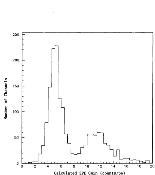
Analyzing the calibration data from January 2003, the outer detector photomulti-plier tubes show a bimodal distribution in Figure 2-3, one centered at approximately five counts per photoelectron, the other centered between eleven and twelve counts. The bimodality is a result of the difference between new and old photomultiplier tubes. After an accident which ruined a number of PMTs in the Super-Kamiokande detector, the burned out tubes were replaced. These new tubes were set to have

4.5 A V <n>ob vs Occupancy 0 0.1 0.2 0.3 0.4 0.5 0.6 0.7 0.8 0.9 1 Occupancy H

Figure 2-2: The mean number of photoelectrons per observed hit against the occu-pancy. For occupancies less than 0.18, the mean for observed hits is less than 1.1.

consistently lower gains than the older tubes, causing non-uniform responses among the photomultiplier tubes.

250 200 V, r-4 0 15Q a. o 50 n4 0 2 4 6 8 10 12 14 16 18 20

Calculated SPE Gain (counts/pe)

Figure 2-3: A histogram showing the distribution of spe gains over the photomultiplier tubes in January 2003. Peaks corresponding to the old and new PMTs are distinctly visible.

22

---Chapter 3

Outer Detector Dark Noise

Calibration

Due to the length of time required for the laser calibration, it became useful to develop a shorter approximate calibration procedure. Although it would not be as exact, the approximate calibration would be good enough to detect problems in calibration drift and possibly for use in correcting the problem of the old and new PMTs. The dark noise calibration technique was meant to meet these needs.

3.1 Procedure

The time-efficiency of the dark noise calibration comes from the fact that it uses signals that the detector is recording already. Instead of having the detector go through a special calibration run, the dark noise calibration analyzes normal data sets. During the short period of time before an actual trigger, the detector records several microseconds of "dark noise". Because the noise level in the Super-Kamiokande detector is low and the time window between recorded events is small, we assume that any recorded event in the noise time window is caused by a single photoelectron. This makes calculating the approximate single-photoelectron gain as easy as calculating the average of the pedestal-subtracted measurements from the noise time window.

ZEU 200 150 100 50 0 _rn -on

.- or~ Ih~

~DarkNorse

'0000 35000 40000 45000 50000 55000 60000 65000

Figure 3-1: The complete data set for one PMT channel 5 during a calibration run. For the dark noise calibration, only hits between 35000 ns and 45000 ns are included in the calculations. The peak is at the actual trigger, corresponding to the flashes for the laser calibration technique.

3.2 Calculations

For direct comparison between the laser calibration and the dark noise calibration, I first took background noise samples from the January 2003 laser calibration run 021373. Collecting data from a 10000 ns time window before each flash as shown in Figure 3-1, there were there were 867,362 nonzero hits during the time windows on the 1,822 working tubes for the entire run. There were roughly 6000 triggered events on each channel, providing 6000 time windows for data and a total of about 60 ms of dark noise data for each tube. This yields a background rate of hits of

867, 362hits

r =

60

1822hs

60ms x 1822channels

on each channel. The time resolution of the outer detector array is T = 15 ns, so the product rr is very small. If the background hits are assumed to be independent, then Poisson statistics can be applied to the noise data.

Following virtually the same calculations as for the laser calibration technique and taking the mean value of photoelectrons per recorded hit to be < n >= r-r, then the

- 5m time window-4 . .f .

-N"4AVW

*11P-vS

*.i 8_

10MOOsAsim

.',

I

60 50 40 30 20 10 N 0 2.5 5 7.5 10 12.5 15 17.5 20 22.5 25 noisegains

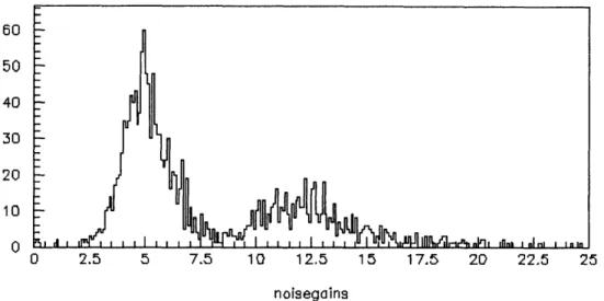
Figure 3-2: The distribution of number of tubes over dark noise gains from the laser calibration run 021373. The distribution here parallels that of the number of tubes over laser calibration gain. The bimodality between old and new tubes is still present.

probability of a nonzero hit having more than one photoelectron is

P(n > > 1 >

) P(r>

P(n > )

1-e

For the calculated value of r = 1.19 x 10- 4_{, this probability is 5.95 x 10}- 5 .

Provided the events are independent, this probability can be ignored. In actuality, the hits are not truly independent, as some of them may be photoelectrons excited by the same incoming particle. In practice, however, the assumption of independence is good enough for the calibration. Ignoring the possibility of n > 1 events, we can take all observed hits to be single photoelectrons.

3.3 Calibration Results

The result of the dark noise calibration, shown in Figure 3-2, using the January 2003 data is similar to that using the laser calibration. The same bimodal distribution is visible, but the curve as a whole is shifted to slightly higher gains. As the dark noise calculations are likely to err on the side of assuming that there are fewer

pho-toelectrons present than there actually are and therefore give a higher gain, this is a sensible result.

The correlation between the laser-calculated gain and the dark noise gain is evident in the linear relation

gainnoise = (0.23 + 0.25) + (1.05 ± 0.04)gaintaser. (3.3)

The line y = 0.23 + 1.05x is shown in the calibration correlation graph.

3.4 Relative Uncertainties and Errors

Using the fit above to relate the two calibration techniques, the dark noise gain and laser gain are within fifteen percent of each other for gains which satisfy

1.15gainilaser > 0.23 + 1.05gainlaer (3.4)

or gains greater than 2.3 counts/spe using the laser technique or greater than 2.6 counts/spe using darknoise. Because this applies to all but a very few extreme outlier tubes, the dark noise calibration technique can be substituted for the laser technique without a loss of accuracy, provided there is enough noise data to ensure a good calibration. The noise calibration is now generally run with ten subruns of data to meet this goal. [6] The ten subruns provide an average of 250 hits for each channel. If the hits were all single photoelectrons, the error in the calibration would be lower than the standard deviation of the average by a factor of

VA,

Dark Noise vs Laser Calibration SPE Gains 25 20 Cn co OI

0.

z

Laser Calibration SPE Gains

Figure 3-3: The graph shows the spe gain determined from the dark noise technique against the gain calculated from the laser calibration. Each dot is one photomultiplier tube. The line is y = 0.23 + 1.05x, the best-fit line to the data.

E

z

0 5 10 15 20 overflow

Dark Noise Hits (counts)

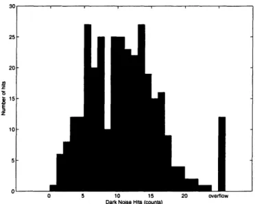
Figure 3-4: A histogram of dark noise hits for PMT channel 5 during run 023219. The gain for this channel was measured to be 11.1 counts/pe, a fairly typical result. If all of the hits were single photoelectrons, the error would be +0.3 counts/pe. Instead, it is taken to be about +1.1 counts/pe.

3.5 Calibration Adjustment Algorithm

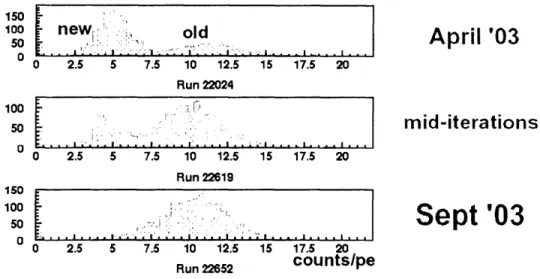
Because the dark noise calibration method is faster than laser calibration and requires no detector downtime while retaining the same amount of accuracy, the dark noise technique has supplanted the laser calibration for the Super-Kamiokande detector. In August 2003, Hans Berns, Bill Kropp, and Kate Scholberg used the dark noise technique to quickly measure the spe gains and determine new high voltages to supply to each PMT, then repeating as necessary to adjust the gains of the new tubes to match those of the old. By September, the gain distribution was no longer bimodal and the average spe gain for all tubes was around eleven counts. [6] The iteration process is depicted in Figure 3-5.

E

...

April '03

mid-iterations

Sept '03

Figure 3-5: The beginning, middle, and end of the adjustment algorithm. The

bi-modal distribution between old and new tubes because a single group. From [6].

150 100 50 0 100 50 0 150 100 50 0 I I

Chapter 4

Stability of Calibration

The final important issue connected to the dark noise calibration is its stability over time. Although the spe gain can be calculated quickly for every data collection run of the Super-Kamiokande detector, knowing the calibration drift over time is important for determining how often adjustments to the voltage settings will need to be made and for determining comparability of data sets from different runs.

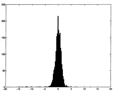
Taking run 023179 (October 12, 2003) as my baseline, I compared later runs to this one. Run 023219, taken three weeks later on November 2, shows little deviation from the baseline. There is a small, even spread on either side of zero drift, as shown in Figure 4-2. The average drift over these three weeks was -0.04 counts/pe.

Comparing over a longer time period, I also looked at run 023975, taken on April 29, 2004. Six and a half months after run 023179, the spe gain had an overall drift of only -0.07 counts/pe. This is especially good compared to the drift in the pedestals over that same time period. Between October and April, the average pedestal drift was -0.36 counts/pe, slightly more than five times the spe gain drift.

I

I

z

SPE Gain, counts/pe

Figure 4-1: The distribution of channels over spe gains for run 023179 on October 12, 2003. These gains are from after the adjustment algorithm. The peak at zero is from dead tubes.

I

-15 -10 -5 5 10 15

Figure 4-2: A histogram of spe gain drift between October

2, 2003. The tubes are centered very tightly at zero drift.

12, 2003, and November 200 150 100 so -20 20 n O . _ _ . _ , I _ v

I

-20 -15 -10 -5 0 5 10 15 20

Figure 4-3: A histogram of 2004.

spe gain drift between October 12, 2003, and April 29,

250 200 150 100 50 L3JU _ Vow

Chapter 5

Conclusion

The dark noise calibration technique has proven to be quick, easy, and sufficient for the level of accuracy needed in the Super-Kamiokande detector. The single photoelectron gains calculated through dark noise are strongly correlated with those from the normal laser calibration technique, and the improved speed has allowed the collaboration to fix the disparity between the old and new tubes in the outer detector. Finally, the dark noise technique also allows checks on the stability of the calibration, showing that the spe gain has only a small drift, especially compared to pedestal drift.

Bibliography

[1] Becker-Szendy, Bionta, et al. Calibration of the IMB Detector. Nuclear Instru-ments and Methods, A352:629-639, 1995.

[2] The K2K Collaboration. Indications of Neutrino Oscillation in a 250 km Long-Baseline Experiment. Physical Review Letters, 90:041801, 2003.

[3] The Super-Kamiokande Collaboration. Evidence for Oscillation of Atmospheric Neutrinos. Physical Review Letters, 81:1562-1567, 1998.

[4] The Super-Kamiokande Collaboration. The Super-Kamiokande Detector. Nuclear Instruments and Methods, A501:418-462, 2003.

[5] John W. Flanagan. A Study of Atmospheric Neutrinos at Super-Kamiokande. PhD thesis, University of Hawaii, December 1997.

[6] Kate Scholberg. OD PMT Gain Tweaking and Status. Super-Kamiokande Col-laboration meeting talk, November 2003.

[7] Kate Scholberg. SK II Outer Detector Calibration Status. Super-Kamiokande Collaboration meeting talk, June 2003.