HAL Id: hal-03117327
https://hal.univ-lorraine.fr/hal-03117327
Submitted on 21 Jan 2021
HAL is a multi-disciplinary open access
archive for the deposit and dissemination of
sci-entific research documents, whether they are
pub-lished or not. The documents may come from
teaching and research institutions in France or
abroad, or from public or private research centers.
L’archive ouverte pluridisciplinaire HAL, est
destinée au dépôt et à la diffusion de documents
scientifiques de niveau recherche, publiés ou non,
émanant des établissements d’enseignement et de
recherche français ou étrangers, des laboratoires
publics ou privés.
Analysis and stochastic simulation of geometrical
properties of conduits in karstic networks
Yves Frantz, Pauline Collon, Philippe Renard, Sophie Viseur
To cite this version:
Yves Frantz, Pauline Collon, Philippe Renard, Sophie Viseur. Analysis and stochastic simulation of
geometrical properties of conduits in karstic networks. Geomorphology, Elsevier, 2021, 377, pp.107480.
�10.1016/j.geomorph.2020.107480�. �hal-03117327�
Geomorphology, 377: 107480–, 2021 10.1016/j.geomorph.2020.107480
Analysis and stochastic simulation of geometrical
properties of conduits in karstic networks
Yves Frantz
1, Pauline Collon
1, Philippe Renard
2, and Sophie Viseur
3 1Université de Lorraine, CNRS, GeoRessources, F-54000 Nancy, France2Centre of Hydrogeology and Geothermics (CHYN), University of Neuchâtel, CH-2000 Neuchâtel - Switzerland 3Aix Marseille Univ, CNRS, IRD, INRAE, Coll France, CEREGE, F-13545 Aix-en-Provence, France
Abstract Despite intensive explorations by speleologists, karstic systems remain only partially de-scribed as many conduits are not accessible to humans. The classical exploration techniques produce sparse data, leading to various uncertainties about the conduit dimensions, essential parameters for flow simulations. Stochastic simulations offer a possibility to better assess these uncertainties. In this paper, we propose different methods to stochastically simulate the properties (size and shape anisotropy) of karstic conduits on already existing skeletons. These approaches, based on Sequential Gaussian Simulations (SGS), allow taking different conditioning data into account, while respecting the intricacy of the networks. To infer the input parameters, we perform a statistical study of the con-duit dimensions of 49 explored karstic networks, focusing on their equivalent radius and width-height ratio. Thanks to the definition of 1D-curvilinear variograms, we demonstrate the existence of a spatial correlation along the networks, which is even higher when considering independently each conduit. Finally, using ad hoc algorithms implemented for computing both a conduit hierarchy inside karstic networks and a relative position regarding outputs, we find no evidence of an obvious link between these two entities and the studied metrics. The simulation methods are then demonstrated on the karstic network of Arrestelia (Pyrénées-Atlantiques, France), and show the consistency of the proposed approach with the observations made on the explored natural systems.
Keywords Karst Conduit network Conduit geometry Statistics Stochastic simulation
1 Introduction
Karstic systems are characterized by a weathered landscape associated with numerous cavities and a subterranean hydro-graphic network entailing large heterogeneities inside the rock. The water flow can form wide networks of conduits with var-ious geometries and topologies. It is estimated that karsts cover between 7% and 12% of emerged lands but they pro-vide potable water for more than a quarter of the whole hu-man population[Hartmann et al.,2014]. The management
of karst ressources and vulnerability often requires to charac-terize these networks in 3D, but also to simulate flows within their conduits.
The modeled karstic networks commonly serve as support for flow simulations. Some software allow performing flow sim-ulations on discrete conduit networks (e.g., SWMM, Epanet, Modflow-CFP). To obtain good results, the network geometry should be as close to reality as possible. Peterson and Wicks
[2006] found out that a difference of conduit length or
diame-ter of 10% can give statistically significant differences of fluid flow responses. Thus, being able to generate spatially variable conduit dimensions along a karstic network could improve the characterization of its fluid flow behaviour using flow simula-tion.
However, karsts are complex systems which remain only par-tially explored. Indeed, speleologists can only collect data in the accessible parts of the networks. The management of karst resources and vulnerability often requires to characterize these networks in 3D. Tracer tests give interesting information about the fluid flow inside the networks, and enable the estimation
of a rough approximation of their geometry (e.g.,Borghi et al.,
2016;Tinet et al.,2019). Nonetheless, this method can not provide highly detailed information about conduit geometries. Acquiring data on paleokarstic systems is even more challeng-ing. The lack of access to these networks impedes the use of tracers and imposes to rely on other techniques (e.g., well or seismic data analysis), which have their own limitations. Wells provide high resolution data but have a very restricted 3D cov-erage. Seismic data allow the identification of large sinkholes but their resolution hardly enables to identify metric conduits (e.g.,Francesconi et al.,2018).
Thus, for about ten years, various methods have been devel-oped to model karstic networks (e.g.,Pardo-Igúzquiza et al.,
2012; Borghi et al., 2012; Collon-Drouaillet et al., 2012;
Fournillon et al.,2012;Viseur et al.,2014;Hendrick and Re-nard,2016b). A large part of them use stochastic procedures, either in the core of the modeling methods or in the genera-tion of the input parameters, providing an insight about the network uncertainties. Some approaches try to reproduce the physical and chemical processes controlling the karstic net-work formation (e.g.,Kaufmann and Braun,2000;Birk et al.,
2003; Dreybrodt et al., 2005). Other approaches focus di-rectly on the reproduction of the final structures using spatial statistics techniques (e.g.,Fournillon et al.,2012;Viseur et al.,
2014). Simplifications and approximations of the formation processes, combined or not with statistics, have also been de-veloped to propose original modeling approaches (e.g.,Jaquet et al.,2004;Labourdette et al.,2007;Pardo-Igúzquiza et al.,
Hen-drick and Renard,2016b).
The local conduit size is often characterized by the radius of its local section. Several authors use constant values of conduit radius to perform flow simulations. They can set one specific value of radius for all the conduits (e.g,Ronayne,2013), dif-ferent values for each conduit (e.g.,Chen and Goldscheider,
2014) or power law values depending on the conduits hier-archy inside the network: high values in conduits receiving the highest recharge, smaller values in conduits receiving less recharge and widening at each confluence (Vuilleumier et al.,
2013;Borghi et al.,2016). Often, the radius or the parameters controlling the radius distribution are calibrated directly dur-ing the flow simulations to reproduce observed discharge rates at different nodes. In these works the values are set constant in each branch (e.g.,Vuilleumier et al.,2013;Jeannin et al.,
2015).
Given the importance of the radius property (e.g.,Peterson and Wicks,2006), we developed simulation methods designed for generating variable radius along karstic networks. These methods aim to fill dataless parts of the networks. They can be applied both to partially known networks or simulated net-work skeletons. These simulation methods constitute the first contribution of this paper.
Stochastic simulation methods require pertinent input pa-rameters. Defining rules on the equivalent radius and the shape anisotropy properties could help modelers to reproduce real-istic karstic networks from sparse information on the conduit geometries. Thus, the second main contribution of this paper is a statistical analysis of a set of observed karstic networks, which meets two objectives: i) highlighting statistical laws on the equivalent radius and the shape anisotropy (measured by a width-height ratio) of the conduits and ii) studying the spatial variability of these properties along the karstic networks.
Thus, in section 2.1, we present the database of 49 networks used for the statistical analysis. It includes the Arrestelia net-work, which is used as a demonstration case to illustrate the simulation methods. Then, in section 2.2.1, we describe the statistical tools used to analyse the karstic data. They include two innovations. First, a 1D-curvilinear variogram is proposed to quantify the spatial variability of the studied metrics along the networks. Secondly, a new algorithm is proposed to rank the karstic conduits in order to analyse the potential correla-tion between the conduit dimensions and their relative posi-tion in the network. In secposi-tion 2.2.2, we introduce two new approaches for simulating the properties along the karstic net-works. They rely on the classical Sequential Gaussian Simula-tion (SGS) method but are adapted to graph structures such as karstic networks. The first method mainly uses the spatial vari-ability at the network scale, whereas the second one privileges the spatial variability within the conduits. Finally, we present the results of the statistical analysis (Section 3.1) and of both simulation methods (Section 3.2) and discuss their significance and limitations (Section 4).
2 Data and methods
In geomorphology, statistical analyses on curvilinear objects were already done on fluvial systems (e.g.,Horton,1945) and different studies tried to expand it on karstic systems from the 1960s onwards (e.g.,Curl,1966;Howard,1971). Basic metrics like network extent, conduit length, dip, orientation, width, height or equivalent radius were already studied (e.g.,Jeannin,
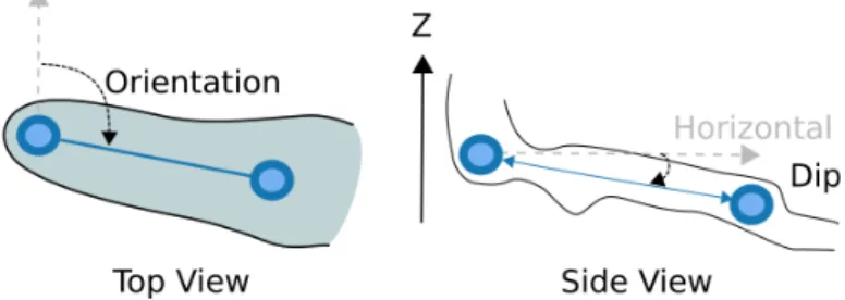
Figure 1 Example of infield measurements of the orientation and dip (modified fromCollon et al.,2017).
1996;Frumkin and Fischhendler,2005;Fournillon et al.,2012;
Collon et al.,2017), but only a few studies focused directly on the statistics of the cross-sectional shape and dimensions of the conduits (Pardo-Iguzquiza et al.,2011;Jouves et al.,2017). We aim here to complement these studies with new karstic networks and additional statistical and spatial descriptors.
2.1 Data
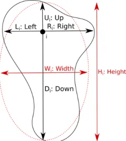
Data acquisition when exploring karstic networks can be quite arduous. Measurements are done at different points called stations, and speleologists determine the distance, orientation and dip between the neighbouring stations (Figure1). With this information, it becomes possible to determine the position of the points in Euclidian coordinates. On some networks, they also measure the width and height at each station or even their 4 dimensions in order to be more precise: right, left, top and bottom (Figure2).
These dimensions are traditionally estimated by sight by speleologists when mapping the networks. This dimensional description is restrictive, for it does not take into account the whole geometry of the conduits but only their main dimensions. The data lack precision, but we nonetheless consider these val-ues as pertinent for our study, as the acquisition methods are similar from a network to another. Nonetheless, new develop-ments in optical laser technology enable better precision since the last decade and adapted rendering methods are currently being developed (e.g.,Lønøy et al.,2020).
To homogenise the values, we choose to estimate the equiv-alent radius (Rei) at a given station i from its width Wi:
Wi= Ri+ Li (1)
and its height Hi:
Hi= Ui+ Di (2)
based on an elliptic approximation (Figure2). We consider each conduit section as an ellipse of the same height and width and define the equivalent radius as the radius of a circle with the same area as the considered ellipse:
Rei=
v tWiHi
4 (3)
To quantify the shape anisotropy, we use the width-height ratio (e.g.,Pardo-Iguzquiza et al.,2011;Jouves et al.,2017) (Figure3):
WHi= Wi
Figure 2 Measurements of the dimensions at a station i of the net-work. The elliptic approximation appears in red.
Figure 3 Schematisation of the width-height ratio.
The data used for this paper consists in 49 different net-works, shared with us by various speleologists during two pre-vious studies (Collon et al., 2017; Jouves et al., 2017) and presented in Appendix A. The extent of these networks can be quite different, the widest one, Sieben Hengste (Switzerland), extending itself over 80 kilometers with 15340 data points, while the smallest one, Baume Galinière (France), has less than 200 meters of conduits with 50 data points. Most of them are rather small, their median length being 2135 meters long, and are sampled with a median number of 269 points. The av-erage sampling distance is every 7.5 meters. It has to be noted that the sampling is not homogeneous and some network parts lack geometrical information. There is also a great uncertainty about the sampling itself.
To perform statistical analyses, networks are represented as graphs[Collon et al.,2017]. They are based on the network
skeletons which correspond to the observed conduits. Each node coincides with a measurement point and holds the width and height information (Figure4). The nodes are linked by edges holding the properties corresponding to the respective lengths and orientations of the conduits. As the direction of the flow within karstic networks are unknown, we use undirected graphs. Undirected graphs are graphs with bidirectional edges, meaning that if there is a direct link between a node A and a node B, there will also be a direct link between the node B and the node A. In opposition, in directed graphs, even if there is a direct link between the node A and the node B, there is not necessarily a link between the node B and the node A. These graphs are cleaned during a first step in order to remove overlapping nodes[Collon et al.,2017].
We can divide the networks into different parts named
Figure 4 Example of a network graph. It corresponds to nodes linked together by edges and is a simple schematisation of the net-work. Both the nodes and the edges can hold information: here nodes hold the width and the height, while edges hold the length, the ori-entation and the dip of the corresponding segments.
Figure 5 Example of branches in a network. Among the seven branches of this network, one is highlighted in blue and another one in red.
branches (Figure5). A branch is defined as a set of adjacent edges connecting nodes, similarly toCollon et al.[2017] and Jouves et al. [2017]. They correspond to the parts located
between two intersections of conduits or network extremities, including the intersections and extremities themselves.
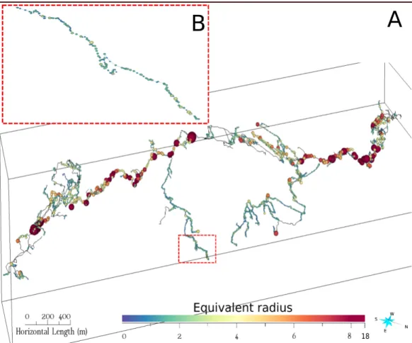
Many aspects covered by the paper are illustrated with the Arrestelia network (Pyrénées-Atlantiques, France, courtesy of J.P. Cassou), which data were post-processed in order to keep only the main explored parts for which the conduit dimensions were available. The data from this 58-kilometers long network are composed of 6000 nodes but only 4283 of them are associ-ated to a radius and a width-height ratio value (Figure6).
2.2 Methods
2.2.1 Statistical inference a) Univariate analysis
Network comparisons
Our first objective is to compare the statistical distributions of the studied metrics in the different networks, to highlight potential similarities. Besides basic statistical analysis, we also use hypothesis testing to achieve this. We perform dif-ferent statistical tests to check the similarities between the net-works, both for the equivalent radius and the width-height ratio. These tests compare the obtained p-value with a cho-senα, the statistical significance (risk of rejecting the tested hypothesis H0 while it is true). If the p-value is inferior to α, the hypothesis H0 is rejected in favour of the alternative
hypothesis H1. Otherwise, there is no clear evidence against the hypothesis H0and it goes unrejected (but is however not validated).
Figure 6 Equivalent radius of the Arrestelia cave in the whole network (A) and in a part of it (B). The size of the nodes is directly proportional to their value.
• The Wilcoxon individual signed rank test to check in-dividually if the distributions of all networks could be samples of a distribution with a specified median (Wilcoxon,1945;Hollander and Wolfe,1999;Gibbons and Chakraborti, 2003). Here we choose to compare them with the median of all network medians.
• The Wilcoxon rank-sum test (which is equivalent to the Mann-Whitney U-test) to compare all the network me-dians two by two by checking if the two distributions could possibly be samples of distributions with the same median (Wilcoxon,1945;Hollander and Wolfe,1999;
Gibbons and Chakraborti,2003).
• The two-sample Kolmogorov-Smirnov test to check if each pairs of networks are likely to be samples originat-ing from the same distribution (Massey,1951;Miller,
1956;Marsaglia et al.,2003).
• The Kruskal-Wallis test to check if each pairs of networks are likely to be samples originating the same distribution (Kruskal and Wallis, 1952; Gibbons and Chakraborti,
2003). It is an extension of the Wilcoxon rank-sum test.
Variographic analysis
The second objective of the statistical analysis is to check if the data are spatially correlated. We hence propose to use variography to characterize the spatial variability along the karstic networks.
Variograms are mathematical functions describing the spa-tial variability of a given random variable. They can be om-nidirectional or computed along a specific direction. The
ex-perimental variogram of a random function Z is computed as follows: γe(h) = 1 2N(h) N(h) X i=1 [Z(xi) − Z(xi+ h)]2 (5)
Where h is a distance and N(h) the number of node pairs distant of h .
Variograms may be computed in a one-, two- or three- mensional space. They are usually computed in the three di-mensional XYZ Cartesian space, but for reservoir applications, it is often necessary to compute them within a UVW paramet-ric space allowing to quantify spatial correlations along the geological structures[Mallet, 2002]. For karst applications,
we would like to compute a variogram along the graph rep-resenting the karstic network, which can not be considered simply as a one-dimensional or a three-dimensional space. Us-ing variograms computed in a Cartesian system of coordinates,
Pardo-Iguzquiza et al.[2011] showed that the width, height
and shape anisotropy are spatially correlated with a corre-lation length of roughly 40m. Here, we refine this analysis and consider the spatial correlation along the conduit network. Therefore, the variograms are computed as 1D-curvilinear var-iograms. Similar approaches were proposed for the case of rivers (Ver Hoef et al., 2006; de Fouquet, 2006). The vari-ograms used during the present study are based on the shortest curvilinear distance between pairs of nodes and are indepen-dent of any specific direction. We use the Dijkstra algorithm [Dijkstra,1959] to compute these distances.
The spatial variability of the studied metrics can also be vi-sually assessed and seems even greater inside the branches
themselves. On the other hand, abrupt differences can be seen at some of the intersections of different conduits (Figure7). To analyse this behaviour, we define the intrabranch variogram, which is only based on pairs of nodes located inside the same branch (Figure8C). We similarly define the interbranch var-iogram, which is based on pairs of nodes located in different branches (Figure8D). In opposition, variograms computed in-dependently of the branches are designed as global variograms (Figure8E).
Metric distribution analysis
Our third objective is to analyse the networks individually, to highlight specific behaviour. To do so, we check if the metric distributions are following a specific parametric law, either a log-normal or a Pareto distribution. Different tests are also used to this end. These tests are designed for uncorrelated data and were therefore performed after the variographic analysis in order to be able to subsample nodes that are sufficiently far away to minimize spatial correlation effects.
• Theχ2goodness-of-fit test (Pearson,1900;Gibbons and Chakraborti, 2003) and the One-sample Kolmogorov-Smirnov test (Massey, 1951; Miller, 1956; Marsaglia et al.,2003) withα = 5% to check if the networks follow individually a Pareto law.
• The χ2goodness-of-fit test (Pearson, 1900; Gibbons and Chakraborti,2003), the One-sample Kolmogorov-Smirnov test (Massey, 1951; Miller, 1956; Marsaglia et al., 2003), the Lilliefors test (Lilliefors, 1967; Lil-liefors, 1969; Conover, 1999), the Anderson-Darling test (Anderson and Darling,1952;Anderson and Dar-ling,1954) and the Jarque-Bera test (Jarque and Bera,
1987) withα = 5% to check if the decimal logarithm of the metrics follow a gaussian distribution.
b) Multivariate analysis
As univariate analyses can not grasp potential links between the studied metrics and other parameters, we have to rely on multivariate analysis.
Relations with the node altitudes and the conduit dips and orientations
Altitudes and conduit dimensions are studied jointly to see if any relation can be observed. As networks form preferentially along pre-existing fracture networks, we compare the dips and orientations of the conduits with their geometrical properties. We could, indeed, expect to see different geometries of conduits depending on the associated fracture family. The conduits link two nodes and are of variable lengths. The orientation and dip are directly computed on the the edge, while the related equivalent radius and width-height ratio are the mean of both edge extremities. If one of the edge extremity has no value, the segment is not taken into account.
Conduit hierarchy
In order to distribute conduit equivalent radius on a network with a minimal number of parameters, it was assumed in pre-vious works (Vuilleumier et al.,2013;Borghi et al.,2016) that
the radius can be expressed as a power-law depending on the hierarchy level of the associated conduit in the network. The rationale behind this assumption was that conduit size should scale with the amount of flow that it can carry and therefore, in average, a conduit located downstream should be larger than a conduit upstream (Figure9A, B). In these papers, the hierar-chical level was estimated by accounting for the catchment size for each inlet into the network and propagated downstream.
Here, we want to test the assumption that the conduit size varies along the system with actual data. However, a practical difficulty is that we do not have access to all hydrogeological information for all the conduit networks that we use. In order to make a systematic analysis on all the networks, we were obliged to define the hierarchy in a simple and reproducible manner. This is the reason why we propose a new ranking method that can handle flow separation and loops as observed in the considered networks, and which does not require any information about the catchments of the inlets or the global karstic network which we rarely have as data (Figure9C, D). The hierarchical values propagate from the entries at the top of the network to the exits at the bottom, similarly to a fluid flowing down into the network under gravity constraint (in accord with the epigenic formation of most networks). To sim-plify the algorithm, all nodes of degree 1 (extremity nodes), which refers to nodes with a single neighbour, are considered as entries or exits, depending on the altitude difference be-tween their position and the closest intersection node within the graph. If the extremity node has an altitude superior to the intersection node, we label it as an entry, as the water will flow within the network per gravity. Otherwise, the extremity is labelled as an exit. If a node is deep within the network and should nonetheless be labelled as an entry, we consider it to be an infiltration node directly linked to a real entry and treat it as a normal entry point. When two conduits of value
nAand nBjoin together, the resulting conduit has an value of nA+ nB. When a conduit of value n divides itself into two, both
resulting conduits become of value n/2, which accounts for the separation of the flow (Figure9B). If this "flow" becomes stuck in a low altitude node (in a siphon) it is made to ascend and reach unreached nodes. This uprising is not fully imple-mented and the whole algorithm is thus only adapted to small networks. Once the conduit hierarchical values are computed, it is possible to look for a correlation with the values of the studied metrics at the same point.
Distance to the closest extremity
To complete the analysis of the conduit hierarchy, we look for a direct link between the distance to the closest entry or exit and the studied metrics. In order to be respectful of the network organisation, we use the curvilinear distance along the network instead of a Euclidian distance.
2.2.2 Simulation methods
In the following, we develop two methods based on Sequential Gaussian Simulations (SGS). These methods aim to generate properties, mostly the radius and width-height ratio, inside karstic networks. These properties are generated along the network graphs. It allows the users to fill dataless parts of known networks or to fill entirely some simulated networks.
These methods respect the conditioning data as well as spec-ified geostatistical information (distribution and variogram)
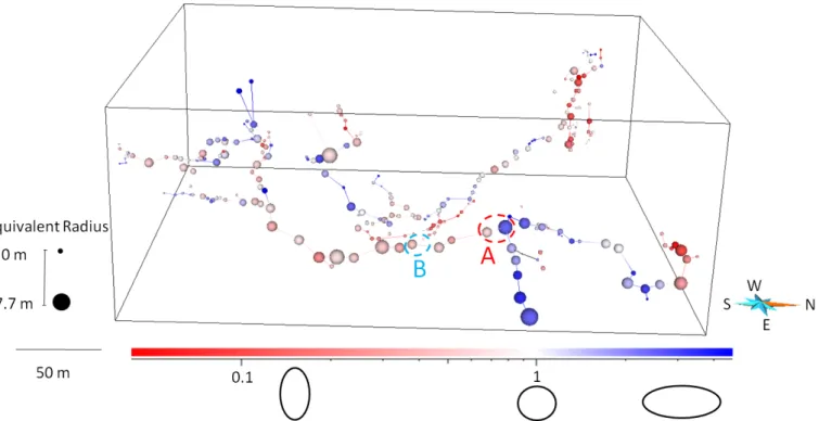
Figure 7 Representation of the Aspirateur network (269 nodes). The size of the nodes is proportional to their equivalent radius while their color depends on the width-height ratio. Noticeable differences between neighbour values can be seen at intersection. A: Difference of width-height ratio. B: Difference of equivalent radius.
Figure 8 A: Example of a network. B: The three branches of this network, each represented by a different color. The intersection node (in grey) belongs to the three branches. C: Nodes (blue) paired with the node 2 (red) during the computation of the intrabranch variogram. D: Nodes (blue) paired with the node 2 (red) during the computation of the interbranch variogram. E: Nodes (blue) paired with the node 2 (red) during the computation of the global variogram. F: List of the nodes paired with the node 2 in C, D and E.
Figure 9 A: Example of a branchwork network which could correspond to a fluvial network or a karstic network. The blue arrows show the direction of the flow and its size is proportional to the theoritical flow value. B: Example of complex network, with one loop and two exits, which could correspond to a karstic network. C-D: Proposed ranking method (top view) applied, respectively, to networks A and B.
while taking the uncertainties into account thanks to their stochastic nature (multiple equiprobable realisations can be performed) (e.g.,Chilès and Delfiner,2009).
The SGS method supposes an input Gaussian distribution. If it is not the case, it becomes necessary to do a normal score transform of the simulated property to get a normal distribu-tion (Goovaerts,1997;Deutsch and Journel,1998). The var-iogram parameters are then estimated from the transformed property instead of the initial property. Finally, a backward transformation step is done to get the true simulated values.
SGS implies a kriging at each node of the network. The kriging is a linear estimator which estimates the value of a node by using its neighbour information. Since the mean of the distribution is known (and is equal to 0 if the distribution is transformed), we use a simple kriging.
For each realization, a random path allowing to visit all the nodes to simulate (valueless nodes) is generated. For each valueless node, the algorithm searches for its neighbourhood. The neighbourhood corresponds to the set of nodes having a value and located closer than a specified distance. If the neighbourhood is empty, a value is sampled from the marginal distribution. Otherwise, a simple kriging is performed and results in an estimated value Z∗
0and its variance of estimation σ2
k. A random value is then obtained using a Monte-Carlo
sampling in the Gaussian distribution N(Z0∗,σ2
k). The result is
added to the conditioning nodes.
The main differences between our methods and the classi-cal SGS methods are: i) the use of the curvilinear distance along the network instead of the Euclidean distance and ii) the definition of the neighbourhood. Besides the distance and the existence of an associated value, the presence of the neigh-bours in the same branch or in a different one as the simulated node is also considered.
Two variants of the 1D-curvilinear SGS are implemented and tested. Both use a distance matrix computed on all pairs of nodes with the Johnson’s algorithm[Johnson,1977]. The
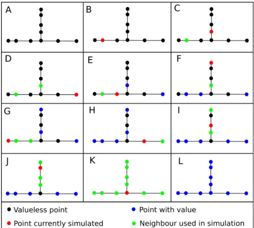
first one respects the spatial variability inferred at the network scale. The algorithm is illustrated in the box entitled Algorithm 1. It simulates all the values using the global variogram. The Branchwise 1D-curvilinear SGS (see Algorithm 2) accounts for the difference in spatial variability within the branches and also try to reproduce the variability at the network scale. It starts by simulating a number of nodes in each branch with the interbranch variogram (Figure 10B-D). The number of simulated nodes in each branch depends on two user defined parameters: a proportion and a maximal number per branch. The remaining nodes located inside the branches are simulated with the intrabranch variogram in a second step (Figure10E-J). The used neighbourhood is, this time, only composed of nodes located in the same branches as the simulated nodes. Finally, the intersection nodes are simulated with the global variogram in a third and last step (Figure10K).
The two methods are implemented in C++ in the RingKarst Plugin of the SKUA-Gocad software1.
3 Results
3.1 Statistical inference
3.1.1 Univariate analysisNetwork comparisons
We first compare the distributions of all networks. Most net-works tend to have similar order of magnitudes of equivalent
Figure 10 Example of one unconditional simulation with the Branchwise 1D-curvilinear SGS. The simulated node order is drawn randomly at each step. As the simulation progress, simulated nodes are used as conditioning data for the following node simulations. A: Initial network. B-D: Interbranch conditioning. Simulation of one node per branch using the interbranch variogram. E-J: Intrabranch simulation. Simulation of all valueless non-intersection nodes using the intrabranch variogram. K: Intersection simulation. Simulation of the intersection node using the global variogram. L: Final result.
Algorithm 1 1D-curvilinear SGS
Input: Network skeleton, distribution, 1D-curvilinear variogram, conditioning data (if conditional simulation) Output: Simulated property values
if distribution not gaussian then
Normal score transform of the distribution and conditioning data
end if
Computation of the shortest curvilinear distance between all pairs of nodes by using the Johnson algorithm
for each realization do
Generation of a random path to visit all the valueless nodes
for each node in the path do
Search for its neighbourhood
if empty neighbourhood then
Draw a random value from the marginal distribution
else
Simple kriging with the global variogram at the node to obtain the expected value Z∗
0and the variance of estimation σ2
k
Sample the normal distribution N(Z0∗,σ2
k) to obtain the node value
Add the result to the conditioning nodes
end if end for
if normal score transform was performed then
Reverse transformation of the results
end if end for
Algorithm 2 Branchwise 1D-curvilinear SGS
Input: Network skeleton, distribution, intrabranch 1D-curvilinear variogram, interbranch 1D-curvilinear variogram, conditioning
data (if conditional simulation), proportion of nodes simulated per branch with the interbranch variogram, maximal number of nodes simulated per branch with the interbranch variogram
Output: Simulated property values if distribution not gaussian then
Normal score transform of the distribution and conditioning data
end if
Computation of the shortest curvilinear distance between all pairs of nodes by using the Johnson algorithm
for each realization do Interbranch conditioning for each branch do
Compute the number of nodes that are to be simulated in this branch from the number of non-intersection nodes in this branch, the input proportion and the maximal number of nodes per branch
Generation of a random path on the same number of valueless non-intersection nodes located inside the branch
for each node in the path do
Search for its neighbourhood
if empty neighbourhood then
Draw random value from the marginal distribution
else
Simple kriging with the interbranch variogram at the node to obtain the expected value Z0∗and the variance of estimationσ2
k
Sample the normal distribution N(Z∗
0,σ2k) to obtain the node value
Add the result to the conditioning nodes
end if end for end for
Intrabranch simulation
Generation of a random path to visit all the valueless non-intersection nodes
for each node in the path do
Search for its neighbourhood in the same branch
if empty neighbourhood then
Draw a random value from the marginal distribution
else
Simple kriging with the intrabranch variogram at the node to obtain the expected value Z∗
0 and the variance of
estimationσ2 k
Sample the normal distribution N(Z0∗,σ2
k) to obtain the node value
Add the result to the conditioning nodes
end if end for
Intersection simulation
for each valueless intersection node do
Search for its neighbourhood
if empty neighbourhood then
Draw a random value from the marginal distribution
else
Simple kriging with the global variogram at the node to obtain the expected value Z∗
0and the variance of estimation σ2
k
Sample the normal distribution N(Z0∗,σ2
k) to obtain the node value
Add the result to the conditioning nodes
end if end for
if normal score transform was performed then
Reverse transformation of the results
end if end for
radius (Figure11) and width-height ratio but, differences are observable from a network to another.
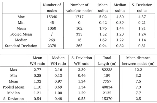
A summary of the raw data can be found in Table1. The pooled mean of the equivalent radius is equal to 1.52 meters, while the pooled mean of the width-heigh ratio is 1.10. The median of the medians of the equivalent radius in the different networks is equal to 1.22 meters and it is equal to 1.00 for the width-height ratio. Detailed statistical values can be found in Appendix A and all histograms are provided in supplementary materials.
The visual inspection of all the histograms reveals a strong asymmetry of the distributions for all cave networks and rather similar shapes of the distributions if we use a logarithmic scale.
The statistical tests are performed on the whole samples, during a blind-study. The Wilcoxon individual signed rank tests are rejected in almost all cases, the exception being the networks with medians extremely close to the median of the medians, both for the equivalent radius and width-height ratio. The results of the other tests are summarized in Table2for the equivalent radius and Table3for the width-height ratio.
As almost all tests are rejected and given the differences observed between the networks (Figure11), we can assume that there is no generic distribution, both for the equivalent radius and the width-height ratio. We thus advise to use, if possible, data acquired specifically on the studied system to define the reference distribution of the modeled network.
Variographic analysis
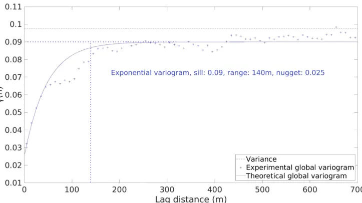
Let us now try to quantify more precisely the spatial vari-ability. When the networks have enough nodes (more than 100), most of the experimental variograms of the decimal log-arithm of the equivalent radius have a behaviour close to the one shown in Figure12. In the other cases, the variograms are far too erratic to be correctly interpretable. The ranges and sills of the variograms differ from a network to another, but the gamma values are usually low at short distance, demonstrat-ing a good spatial correlation between close nodes. There is still a nugget effect which can not be avoided given the usual data sampling (one data point every 7.5 meters in average on the studied networks). After a sharp increase, the experi-mental variogram values oscillate around the sill value, which means that the data become spatially independent. In most cases, exponential models of variograms represent well the experimental variogram. We also often observe an interme-diate stabilization of the variogram. This could be modeled with nested variograms, which are the combination of multi-ple variogram models, and the high distances only concern few data nodes. It could be interpreted as two scales of variability, which is likely a direct consequence of the network intricacy. Nonetheless, for the sake of simplicity we decide to keep only one single structure.
While we observe a low spatial variability of the radius and of the width-height ratio inside the networks, the variability of the metrics is even lower inside the branches: the intrabranch variogram has values lower than the global variogram (Fig-ure13). Conversely, two nodes located in different branches are likely to have more different values than two nodes in the same branch, even at close distance. The interbranch vari-ogram values are higher than the global varivari-ogram values at close distance. This underlines an important spatial variability between the different branches. Since the branches have a very
limited size, the values of the intrabranch variograms become quickly erratic because of the lack of data pairs. Finally, the interbranch variogram starts to overlap with the global vari-ogram past a certain distance (wich is usually proportional to the size of the network).
These results highlight the spatial variability of the studied metrics inside the networks and their branches and constitute a good basis to perform stochastic simulations.
Metric distribution analysis
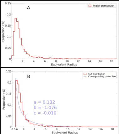
We also check if the distributions of the network metrics follow a specific law. On a logarithmic scale, the histograms obtained for most of the large networks seem close to normal (Figure14), both for the radius and for the width-height ratio. Narrow conduits tend to be undersampled and it is hard to make measurements on vertical conduits. It leads to an un-derestimation of small values, both for the equivalent radius and the width-height ratio. It is one of the reasons behind the log-normal aspect of the distribution and leads also to mislead-ing representations of the distributions on a linear scale. Thus, after truncating the distributions above its smallest values to try to remove the sampling bias, they seem to follow a Pareto law or a Power law on a linear scale (Figure15).
We first performed the different tests on the whole networks in a blind approach and most of them were rejected. Yet, these tests could not be truly considered as valid as the different node values are not independent from each others, as demonstrated by the variographic analysis. For that reason, we perform the tests on subsampled networks, where all kept nodes are more distant from each others than the global variogram range. As we desire to perform these tests on more than a few points, we subsample only the 11 networks which have 1000 data points or more. The subsampling is done twice, both for the equiva-lent radius and for the width-height ratio, because the ranges of their variograms are usually different. The resulting uncor-related subsamples have thus a mean number of 53 points (as the range of the variograms can be important). The results can be found in Table4for the Pareto distribution and Table5for the log-normal distribution.
The results seem to indicate an absence of a strong bias against the existence of a Pareto or a log-normal distribu-tion, both for the equivalent radius and the width-height ra-tio. Nonetheless, given the incompatibility between these two distributions, the small number of subsampled networks and their small number of associated values, it is not possible to over-interpret these results. Even if the visual inspection of the 49 histograms shows that those computed on large networks are close to being log-normal, the statistical tests can not fully confirm this hypothesis. A power-law may also be representa-tive of the equivalent radius distributions but the lack of small values in our data do not allow to prove it either.
3.1.2 Multivariate analysis
Relations with the node altitudes
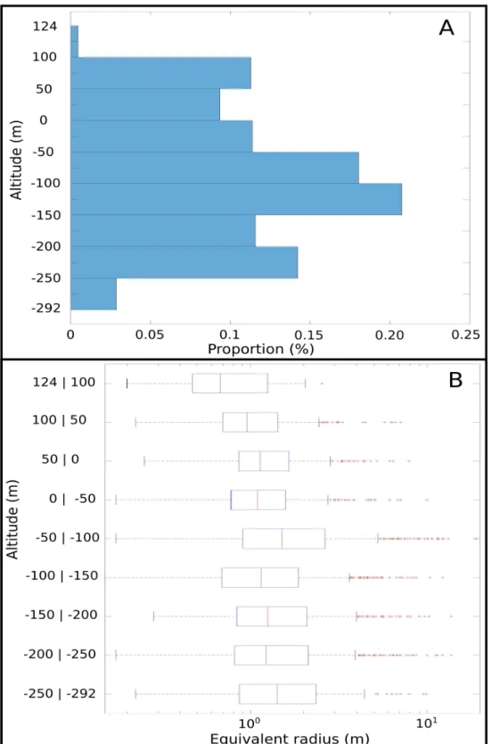
We now look for a relation between the node altitudes and their associated geometrical properties. Figure 16A shows the distribution of the altitudes within the Arrestelia network, while Figure16B shows the boxplot of the equivalent radius for different ranges of altitudes. This example is representative of the results we obtain on almost all studied karstic systems
Number of nodes Number of valueless nodes Mean radius Median radius S. Deviation radius Max 15340 1717 5.02 4.80 4.37 Min 45 0 0.42 0.39 0.21 Mean 1050 102 1.76 1.44 1.31 Pooled Mean / 333 1.52 1.20 1.24 Median 269 16 1.62 1.22 1.14 Standard Deviation 2378 265 0.94 0.82 0.81 Mean WH ratio Median WH ratio S. Deviation WH ratio Total Length (m) Mean distance between nodes (m) Max 2.77 2.16 3.39 82238 12.2 Min 0.25 0.13 0.46 189 3.2 Mean 1.32 0.97 1.34 7757 7.5 Pooled Mean 1.10 0.69 1.34 40834 7.3 Median 1.21 1.00 1.29 2135 7.7 S. Deviation 0.54 0.48 0.55 15370 2.5
Table 1 Summary of the statistical analysis of the raw data of 49 different networks.
Figure 11 Boxplot of the of the equivalent radius in the different networks. We use a logarithmic scale for the y-axis. The boxes correspond to to the interval between the first and the third quartile, while the red strike corresponds to the median value. The zone between the whisker extremities represent around 99% of the values, the other ones being outliers.
Figure 12 Experimental and theoretical variograms of the equivalent radius decimal logarithm for the Arrestelia network (4283 data nodes). We decide to limit the display to a maximal plotted distance of 700 meters but the maximal distance is close to 2000 meters.
Figure 13 The 3 experimental variograms of the equivalent radius decimal logarithm for the Arrestelia network (4283 data nodes), along with the corresponding theoretical variograms. Also, after 350 meters, the values of the intrabranch variogram become too erratic to be considered as valid.
α 5% 10% 20% Wilcoxon rank-sum 0.84 0.86 0.90 Kruskal-Wallis 0.84 0.87 0.90 Two-sample Kolmogorov-Smirnov 0.91 0.93 0.95
Table 2 Proportion of rejected tests of network similarity for the equivalent radius depending on the statistical significance.
α 5% 10% 20%
Wilcoxon rank-sum 0.84 0.86 0.89 Kruskal-Wallis 0.84 0.86 0.89 Two-sample Kolmogorov-Smirnov 0.89 0.92 0.94
Table 3 Proportion of rejected tests of network similarity for the width-height ratio depending on the statistical significance.
Figure 14 Histogram of the decimal logarithm of the equivalent radius in the Arrestelia network (4283 data nodes), along with an adjusted gaussian distribution.
Figure 15 A:Histogram of the equivalent radius in the Arrestelia network (4283 data nodes). B: Histogram of the equivalent radius in the Arrestelia network without the values inferior to 0.6 (3573 data nodes). A power-law is adjusted to this cut distribution: f(x) = 0.132∗ x−1.076− 0.010.
: no clear relation between the geometrical properties of the conduits and their altitudes is observed in the different net-works. Nonetheless, some networks have smaller values of radius associated to high altitude nodes (e.g., Figure16B), but it is likely because they correspond to the vadose parts of the networks, where conduits tend to be narrower (Jouves et al.,
2017). It is, however really case dependent and should not be generalized for unexplored networks. Moreover, discussions with speleologists have warned us about the diversity of height and width definitions in sub-vertical conduits, which are, in practice, less sampled.
Relations with the conduit dips and orientations
We then analyse the relation between the conduit dips and orientations and their geometries. Most networks, such as Ar-restelia do not seem to present any generic relation between the conduit dips and orientations and the studied metrics (Fig-ure17). Yet, it exists in some specific networks (Figure18). As a consequence, no generic relation can be drawn for all karstic networks. But it seems that in some particular cases, probably when pre-existing fractures are involved in the speleogenetic process, relations can be identified. Such relation should, how-ever, be first demonstrated in the specific studied context as in some cases, even with preferred orientation developments, no relation appears (e.g. Figure17).
Conduit hierarchy
We now illustrate the results obtained with the hierarchical ranking method. Figure19A shows an example of the
com-Figure 16 A: Histogram of the altitudes of the Arrestelia network nodes (4283 nodes, only those associated to an equivalent radius value are taken into account). B: Boxplot of the equivalent radius depending on the altitudes values.
Figure 17 A: Rose diagram of the Arrestelia network conduit segments (6012 segments). B: Schmidt net of the Arrestelia network conduit segments (6012 segments). C: Histogram of the orientations of the Arrestelia network conduit segments (4009 segments, only those associated to an equivalent radius value and which are not vertical are taken into account). D: Histogram of the dips of the Arrestelia network conduit segments (4088 segments, only those associated to an equivalent radius value are taken into account). E: Boxplot of the equivalent radius depending on the orientation values. F: Boxplot of the equivalent radius depending on the dip values.
Figure 18 A: Wakulla network (474 nodes). The size of the nodes is proportional to the associated equivalent radius. There seem to be a clear difference of behaviour between the North-South conduits and the East-West conduits. B: Histogram of the orientations of the Wakulla network conduit segments (469 segments, only those associated to an equivalent radius value are taken into account). C: Boxplot of the equivalent radius depending on the orientation values.
Equivalent radius WH ratio
χ2goodness-of-fit test 0.27 0.27
One-sample Kolmogorov-Smirnov test 0.55 0.18
Table 4 Proportion of rejected tests checking if the distributions follow a Pareto law on the 11 uncorrelated subsamples, forα = 5%.
Equivalent radius WH ratio
χ2goodness-of-fit test 0.09 0.36
One-sample Kolmogorov-Smirnov test 1 0.82 Lilliefors test 0 0.27 Anderson-Darling test 0.09 0.36 Jarque-Bera test 0.09 0.36
Table 5 Proportion of rejected tests checking if the distributions follow a log-normal distribution, on the 11 uncorrelated subsamples, for
α = 5%.
puted hierarchical values on the Everest network. This network is indeed one of the most simple karstic network we have, with sufficiently few siphons to allow a consistent ranking when no flow direction information are available. Figure19B shows the boxplot of the equivalent radius for different levels of hierarchy. We see a slight increase of the radius for the highest hierarchi-cal values but no clear regular increase of the radius with them, and the high values only concern few data nodes. Moreover, a visual inspection (for example in Figure7) of the networks shows that the radius varies in a complex manner in space, as large radius can be found anywhere along the network. They do not seem to increase with the hierarchy level in a simple manner.
Distance to the closest extremity
To complete this ranking analysis, we study the link between the distance of the nodes to the closest exits and entries defined by our algorithm and its radius and width-height ratio. This approach is interesting as it can be applied even on complex networks with siphons. The Figure20shows the results for the Arrestelia network on which no direct relation between the distance to the closest exit and the radius of the conduits is underlined. The shown bins and boxes have a width equal to 50 meters but the same results are observed for lower widths. No relation is also found for the width-height ratio. Similar results are observed in the different networks.
3.2 Property simulation
3.2.1 1D-curvilinear SGSWe use the Arrestelia network as a basis to illustrate and test the proposed simulation method. The average distance between each measurement station is 9.7 meters but since the sampling is not regular, we choose to densify the network with a maximal distance of 5 meters. The distance of 5 meters is chosen to have enough data nodes to perform a robust analysis of the simulation results, while keeping a reasonable computation time. The network used for simulation tests has thus 14610 nodes, with 4283 holding geometrical information.
Twenty unconditional simulations of the decimal logarithm of the equivalent radius are performed on the whole Arrestelia
network (e.g. Figure21). We choose to perform the simula-tions on the decimal logarithm of equivalent radius instead of the metrics themselves, as its variations are less important. We use the distribution of the decimal logarithm of the equivalent radius of the Arrestelia network as an input parameter. The in-put variograms are comin-puted on the property obtained with the normal score transform of the decimal logarithm of the equiv-alent radius of the Arrestelia network (because the distibution is not gaussian). We choose a maximal size of neighbourhood of 16 nodes to limit the computation time.
The distributions of the results are rather close to the initial distribution but they are more centred around the mean (Fig-ure22). Nonetheless, the means and the medians are close: the mean of the results is 0.10 instead of 0.095, while the me-dian of the results is 0.084 instead of 0.073. The variances are a bit lower than the initial ones, with an average value of 0.092 instead of 0.097.
While the experimental global and interbranch variograms computed on the simulations are close to the input one, it is not the case for the intrabranch variogram, which is closer to the other variograms (Figure23). Since it is not used in that simulation method, this result was expected.
We also perform 20 conditional simulations (e.g. Figure24). We create the conditioning data randomly by choosing random nodes distant of more than 100 meters from each other, 203 in total. We then perform a Monte-Carlo sampling of 203 ran-dom values in the initial distribution, assign them ranran-domly to these nodes and use them as conditioning data. The input dis-tribution variograms and maximal size of the neighbourhood are the same as for the unconditional simulation.
The statistical values of the results are almost similar to those of the unconditional simulations with a mean value of 0.10, a median of 0.080 and a variance of 0.091. It is also the case for the histograms and variograms (Figures25;26).
A brief summary of the results can be found in Table6.
3.2.2 Branchwise 1D-curvilinear SGS
We perform 20 unconditional simulations of the decimal loga-rithm of the equivalent radius on the Arrestelia network using the Branchwise 1D-curvilinear SGS (e.g. Figure27). The in-put distribution variograms and maximal size of the neighbour-hood are the same as for the first method. After testing different
Figure 19 A: Hierarchisation of the conduits inside the Everest network (94 nodes). The size of the nodes is directly proportional to their value. B: Boxplot of the equivalent radius depending on the hierarchisation values of the nodes.
Figure 20 A: Histogram of the distance to the closest exit within the Arrestelia network (4283 nodes). B: Boxplot of the equivalent radius depending on the distance to the closest exit within the Arrestelia network.
Figure 21 A: Part of the initial network. B-C-D: 3 Examples of results obtained on this part during a simulation by unconditional simulation with the 1D-curvilinear SGS method on the whole network (no conditioning data are used).
Figure 22 Histogram of the sum of 20 unconditional simulation results obtained with the 1D-curvilinear SGS method, along with the initial distribution of the decimal logarithm of the equivalent radius.
Mean Median Variance Data 0.095 0.073 0.097 Unconditional simulation results 0.10 0.084 0.092 Conditional simulation results 0.10 0.080 0.091
Table 6 Comparison of input parameters and results of 20 simula-tions performed using the 1D-curvilinear SGS method.
values of proportion and maximal number of nodes simulated using the interbranch variogram in each branch during the pre-conditioning step, we observe that the most satisfying results are obtained with a maximal number of 15 nodes and a pro-portion of 100%. It means that if a branch has more than 15 valueless nodes, 15 of them are simulated with the interbranch variogram and the others are simulated with the intrabranch variogram (Algorithm2). Otherwise, all of them are simulated with the interbranch variogram.
The distributions of the results are close to the initial dis-tribution but less than with the previous method (Figure28). Nonetheless, the means and the medians are closer to those of the data than with the previous method: the mean of the re-sults is 0.098 instead of 0.095, while the median of the rere-sults is 0.081 instead of 0.073. The values are nonetheless more centred around the mean and median values, because of an important decrease of the variance from 0.097 to 0.078.
Since the intrabranch variogram contributes more than pre-viously, and that its sill is lower than the global sill, it is but natu-ral to observe a lower resulting variance. This phenomenon can be observed in the computed variograms (Figure29). The in-trabranch variogram tends indeed to be more respected (even if the fit is still perfectible) but the values of the general and interbranch variograms are significantly lower than the data. The differences between the intrabranch variogram and the interbranch and global variograms are now clearly visible.
We also perform conditional simulations and the overall statistics of the results are also close to those of the uncon-ditional simulations, as seen in Table7.
Figure 23 Mean experimental variograms of 20 unconditional simulation results obtained with the 1D-curvilinear SGS method, along with the theoretical variograms of the decimal logarithm of the equivalent radius.
Figure 24 A: Part of the initial network. B-C-D: 3 Examples of results obtained on this part by conditional simulation with the 1D-curvilinear SGS method on the whole network (use of conditioning data).
Mean Median Variance Data 0.095 0.073 0.097 Unconditional simulation results 0.098 0.081 0.078 Conditional simulation results 0.098 0.084 0.078
Table 7 Comparison of input parameters and results of 20 simulations performed using the Branchwise 1D-curvilinear SGS method
Figure 25 Histogram of the sum of 20 conditional simulation results obtained with the 1D-curvilinear SGS method along, with the initial distribution of the decimal logarithm of the equivalent radius.
4 Discussion
4.1 Statistical analysis
The present statistical analysis is performed on a large database of karstic networks. No other similar study was, to our knowl-edge, done on that many networks so far. Except for small differences, mostly linked to the cleaning of the networks, the mean width-height ratio of the different networks are similar to those presented inJouves et al.[2017] andPardo-Iguzquiza et al.[2011].
We show that there is no single and universal simple sta-tistical law that can be applied anywhere regardless of local conditions to describe the distributions of the equivalent radius and width-height ratio. Statistical tests are performed in order to assess our observations, but the existence of a distribution identical in all networks is rejected. Nonetheless, most of these networks are located in the same regions and some are likely parts of the same systems, which may induce bias.
Tests performed on uncorrelated subsamples do not reject the assumptions that the distributions of the large networks are simply log-normal or of Pareto type. As these tests are per-formed on only 11 subsamples, which are themselves small (mean number of 53 values), it is, however, difficult to ex-trapolate the results. There is also no obvious reason why a Gaussian or Pareto distribution should represent perfectly the reality of the equivalent radius. Indeed, the data are directly measured by speleologists, mostly on human-sized conduits. It means that the conduits of smaller dimension are not taken into account in these data. Given the fractal behaviour ob-served in some networks (e.g.,Hendrick and Renard,2016a) and which may be generalized in most cases (Pardo-Igúzquiza et al.,2019), the real distributions of conduit equivalent radius may be more likely to follow a power-law.
Because of the complexity of the networks, measurements may lack precision, which directly impacts the results of the
analysis. The elliptic approximation is also a potential source of errors on the results. It tends to smooth the shape of the con-duits (hence the "approximation"). Yet, we assume that there is no basic approximation as close to the reality as this one. A circular or rectangular approximation would be less respectful of the shape of the conduits. Nonetheless, the cumulation of the distance in two directions to get the width and the height changes the centering of the conduits. Moreover, the cleaning of networks (e.g., removal of duplicated nodes) implies neces-sary hypotheses, which may also constitute a source of errors. However, flow simulators (e.g., SWMM, Epanet, Modflow-CFP) only consider such approximation of the conduit shape. Thus, this treatment is consistent with the fact that we aim to provide a mean to compute this equivalent property and not the exact geometry of the conduits.
No generic relation between the node altitudes, the conduit orientations or their dips and the conduit geometrical proper-ties are found. Yet, there seems to be existing links in some networks. We thus advise for case-by-case analysis. The defini-tion of the conduit width and height are also difficult to define for almost vertical conduits.
The ranking algorithm is thought to obtain values equiva-lent to a theoretical flow within the networks and handles the presence of loops and the existence of more than one exit for most networks. It is currently usable only for small networks because of the difficulties to handle siphons, but no link is found between the studied metrics and the computed conduit hierarchy. Borghi et al. [2016] associate each conduit with
a value proportional to the supposed corresponding drained area. The drained areas are computed from the topography and are linked to each inlet of the network. If we had the corresponding topological information, it would be interesting to use these values instead of assigning a value of 1 to each potential inlet. It is nonetheless complicated to define an effi-cient ranking method as the water flow within the networks can change depending on different parameters. The lack of general information about the potential entries and exits and the fact that the networks are usually not fully mapped are also major problems. Despite these difficulties, the visual in-spection of the data show that there is no simple hierarchy in the distribution of the conduit. This leads us to question this assumption for defining the conduit radius, which, it should be mentioned, is not based on field data.
No direct link between the distance to the closest exit or entry and the conduit geometrical properties were found during this study. It also brings doubt about the idea of conduit becoming wider, the farther they are within the network, with maximal values associated to the springs. As the network can have many entries and exits (or at least termination nodes), the biggest equivalent radius is not necessarily associated to a specific exit conduit.
Moreover, it can be hard to define where are the entries and the exits of the network. The main entries and exits may be
Figure 26 Mean experimental variograms of 20 conditional simulation results obtained with the 1D-curvilinear SGS method, along with the theoretical variograms of the decimal logarithm of the equivalent radius.
Figure 27 A: Part of the initial network. B-C-D: 3 Examples of results obtained on this part by unconditional simulation with the Branchwise 1D-curvilinear SGS method on the whole network (no conditioning data are used).
Figure 28 Histogram of the sum of 20 unconditional simulation re-sults obtained with the Branchwise 1D-curvilinear SGS method along, with the initial distribution of the decimal logarithm of the equivalent radius.
known for active networks but is no easy task to determine them for case where this information is not available, such as in paleokarstic networks. Our method to define the entries and exits of the network may not be efficient or realistic but there is no obvious way to define them when the information are not present. Also, the matrix flow is not taken into account, while it is not be negligible in reality. To summarize this part of the work, we consider that this study leads to reject the previous assumption of a dependence of the conduit radius with the hierarchical value or the distance to the exits since it is not supported by the data and shows much more complexity.
The 1D-curvilinear variograms underline existence of spatial correlation at a scale of the equivalent radius and the width-height ratio inside the networks. The variability is usually low inside the branches. The ranges of the variograms differ from a network to another but seem nonetheless higher than in Pardo-Iguzquiza et al.[2011], who computed it with Euclidean
dis-tances. Not taking the curvilinear structure of the networks could, indeed, lead to an underestimation of the spatial corre-lation of the studied metrics.
Nonetheless, intrabranch variograms are limited in range because of the definition of the branches. As a branch is de-fined between two intersection nodes, the real length of the conduit do not matter. If a long conduit is joined in different places by other conduits, only small parts of this conduit will be individually taken into account.
Palmer[1991] proposed the first classification of cave
pat-terns and further studies have offered more detailed informa-tion about them (e.g.,Audra and Palmer,2013). Depending on the type of recharge, the position of the water table and its evo-lution, as well as other parameters (e.g., porosity, lithology), different speleogenesis processes, resulting in the existence of different patterns of network structures, were indeed identi-fied. Networks are usually formed over a long period of time, during which the speleogenesis process may change. Different parts of the same networks can thus be formed through dif-ferent processes.Jouves et al.[2017] underlined differences
of width-height ratio and other metrics between the different cave patterns. Some of the networks in our database were divided into different parts during this work, depending on the associated speleogenesis process. We try to expand this analysis to the equivalent radius of the networks. An overview of the results is presented in Appendix B. As some network studied by Jouves did not have the geometrical information
we needed, the number of networks associated to each pattern may be slightly different. The results of this pattern study offer new information but should not be generalized, as it is not ro-bust. Indeed, we have far too few networks associated to each pattern, they are all located in France and some of them are in fact different parts of the same network, so the real number is even smaller. Moreover, most of these parts are rather small, compared to a full network, meaning that the statistical signif-icance of the analysis is rather questionable. For example, the famous Lechuguilla cave is one of the longest cave of the world and was formed through hypogenic processes (e.g.,Duchene et al.,2017). The 5 hypogenic networks presented in this study appear to have a really small extent and are thus not represen-tative of such a cave. Furthermore, while field information are used to divide the networks in different parts, the division is also based on the topology and geometry of the conduits and may induce a bias. It is logical for conduits in the vadose parts of the network to be more vertical and have smaller width-height ratio. Hence, while these results are interesting, they should not be over-interpreted.
4.2 Simulation
Two approaches are proposed to simulate properties along com-plex karstic networks, while reproducing input statistics and conditional data. Both approaches honor the input distribu-tion. The 1D-curvilinear SGS method reproduces the global variogram. The results are reasonable but the intrabranch vari-ogram is not reproduced. This is not surprising because the al-gorithm does not account for it. The Branchwise 1D-curvilinear SGS method is still not completely satisfactory. It accounts for the intrabranch and interbranch variograms. It partially re-spects the intrabranch variogram, but it induces a lower value of variance in both the general and interbranch variograms, as well as a slightly narrower distribution. Additional work is therefore required to design an algorithm that would properly reproduce both the intrabranch and interbranch variograms.
The main advantages of the proposed simulation methods are:
• They are not based on a regular or cartesian grid. It re-sults in smaller computation times and allows the user to freely define the resolution of the networks. Yet the computation times can still be important for large net-works (around 30 seconds per unconditional realisation to simulate around 15000 nodes on a standard laptop). • They allow to simulate the spatial variability inside one
conduit instead of a constant value for the whole con-duit.
• They use a skeleton defined by the user and there is no dependence between the creation of the skeleton and the generation of its property. It gives the user the choice to work on already explored networks or on simulated networks.
• They are based on observed statistics, instead of arbi-trary values, and input parameters can be specifically defined by the user for each network.
• They are stochastic, which gives a good insight about the network conduit and geometry uncertainties.
Figure 29 Mean experimental variograms of 20 unconditional simulation results obtained with the Branchwise 1D-curvilinear SGS method, along with the theoretical variograms of the decimal logarithm of the equivalent radius.
• It would also be possible to adapt these methods to non-geometrical properties (e.g., porosity), given that a low spatial variability at short range is shown by a 1D-curvilinear variographic analysis. They could also be used to simulate properties on other curvilinear net-works, such as rivers.
5 Conclusion
This paper presents two simulation methods adapted to the case of karstic networks. A statistical analysis of the equivalent radius and width-height ratio of the conduits is done on 49 different networks.
These analysis show the absence of perfectly similar distri-butions for the studied metrics within the different karstic net-works. The distributions are found to be close to log-normal but they would not follow exactly such a distribution. No real link are found between the studied metrics and the altitudes, the conduit orientations and the conduit dips. Besides, the studied metrics are not found to correlate well with the hierar-chical ranks computed in this paper. In addition, the inspection of the data seem to indicate that there is no clear correlation between the hierarchy of the network and the equivalent ra-dius or width-height ratio. No relations are also observed with the distance to the closest entry and exit. Moreover, the low spatial variability of the metrics at short range is highlighted by the development of 1D-curvilinear variograms, and an even lower variability is observed inside the branches.
The developed simulation methods permit to reproduce, at least partially, the intricacy of the networks with the use of geostatistics. These algorithms allow generating an equivalent radius and a width-height ratio closer to actual observations than what is done in previous studies. While the input distribu-tions are respected, the input variograms are not currently per-fectly reproduced when performing unconditional simulations. The 1D-curvilinear SGS method reproduces the global vari-ogram but the behaviour on the branches is not respected. On the other hand, the Branchwise 1D-curvilinear SGS method is
close to reproducing the intrabranch variogram but the global and interbranch variograms have lower values.
Nonetheless, these results are an important step towards the simulation of realistic conduit dimensions. They can be applied for various purposes such as flow simulations within discrete conduit networks (e.g., SWMM, Epanet, Modflow-CFP).
Acknowledgments
The authors are also really greatfull to all speleologists and colleagues who provided the karst data, and particularly : B. Arfib, J. Bodin, J. Botazzi, J-P. Cassou, J-L. Galera, S. Jail-let, P-Y. Jeannin, J. Jouves, T. Kincaid, E. Pardo-Iguzquiza, C. Vuilleumier, the Quintana Roo Speleological Survey. This work was performed in the frame of the RING project2at
Uni-versité de Lorraine. We would like to thank the industrial and academic sponsors of the RING-Gocad Research Consortium managed by ASGA for their support and Emerson-Paradigm for providing the SKUA-GOCAD software and API.
References
Anderson, T. W., Darling, D. A., 1952. Asymptotic Theory of Certain "Goodness of Fit" Criteria Based on Stochastic Processes. The Annals of Mathematical Statistics 23 (2), 193–212. (Cited page6)
Anderson, T. W., Darling, D. A., 1954. A Test of Goodness of Fit. Journal of the American Statistical Association 49 (268), 765–769. (Cited page6)
Audra, P., Palmer, A. N., 2013. The Vertical Dimension of Karst: Controls of Vertical Cave Pattern. In: Treatise on Geomorphology. Vol. 6. Elsevier, pp. 186–206. (Cited page25)
Birk, S., Liedl, R., Sauter, M., Teutsch, G., 2003. Hydraulic boundary condi-tions as a controlling factor in karst genesis : A numerical modeling study on artesian conduit development in gypsum. Water Resources Research 39 (1), 1–14. (Cited page2)
Borghi, A., Renard, P., Cornaton, F., apr 2016. Can one identify karst conduit networks geometry and properties from hydraulic and tracer test data? Advances in Water Resources 90, 99–115. (Cited pages2,3,6, and23)