HAL Id: cea-02339998
https://hal-cea.archives-ouvertes.fr/cea-02339998
Submitted on 17 Mar 2020HAL is a multi-disciplinary open access archive for the deposit and dissemination of sci-entific research documents, whether they are pub-lished or not. The documents may come from teaching and research institutions in France or abroad, or from public or private research centers.
L’archive ouverte pluridisciplinaire HAL, est destinée au dépôt et à la diffusion de documents scientifiques de niveau recherche, publiés ou non, émanant des établissements d’enseignement et de recherche français ou étrangers, des laboratoires publics ou privés.
NEPTUNE_CFD and STAR-CCM+
O. Marfaing, M. Guingo, J. Laviéville, S. Mimouni, E. Baglietto, N.
Lubchenko, B. Magolan, R. Sugrue, B.T. Nadiga
To cite this version:
O. Marfaing, M. Guingo, J. Laviéville, S. Mimouni, E. Baglietto, et al.. Comparison and Uncertainty Quantification of Two-Fluid Models forBubbly Flows with NEPTUNE_CFD and STAR-CCM+. Nu-clear Engineering and Design, Elsevier, 2018, 337, pp.1-16. �10.1016/j.nucengdes.2018.05.028�. �cea-02339998�
Comparison and Uncertainty Quantification of Two-Fluid Models for
Bubbly Flows with NEPTUNE_CFD and STAR-CCM+
O. Marfaing
a, M. Guingo
b, J. Laviéville
b, S. Mimouni
b,
E. Baglietto
c, N. Lubchenko
c, B. Magolan
c, R. Sugrue
c,
B. T. Nadiga
da. Den-Service de thermo-hydraulique et de mécanique des fluides (STMF), CEA, Université Paris-Saclay, F-91191, Gif-sur-Yvette, France
b. Electricité de France R&D Division, 6 Quai Watier, F-78400 Chatou, France
c. Department of Nuclear Science and Engineering, Massachusetts Institute of Technology, Cambridge, MA 02139, USA
d. LANL, Los Alamos, New Mexico 87545, USA
Keywords: Multiphase CFD, Bubbly Flow, Momentum Closures, DNB
Abstract
The nuclear industry is interested in better understanding the behavior of turbulent boiling flows and in using modern computational tools for the design and analysis of advanced fuels and reactors and for simulation and study of mitigation strategies in accident scenarios. Such interests serve as drivers for the advancement of the 3-dimensional multiphase Computational Fluid Dynamics approach. A pair of parallel efforts have been underway in Europe and in the United States, the NEPTUNE and CASL programs respectively, that aim at delivering advanced simulation tools that will enable improved safety and economy of operations of the reactor fleet. Results from a
collaboration between these two efforts, aimed at advancing the understanding of multiphase closures for pressurized water reactor (PWR) application, are presented. Particular attention is paid to the assessment and analysis of the different physical models implemented in NEPTUNE_CFD and STAR-CCM+ codes used in the NEPTUNE and the CASL programs respectively, for
application to turbulent two-phase bubbly flows. The experiments conducted by Liu and Bankoff (Liu, 1989; Liu and Bankoff 1993a and b) are selected for benchmarking, and predictions from the two codes are presented for a broad range of flow conditions and with void fractions varying between 0 and 50%. Comparison of the CFD simulations and experimental measurements reveals that a similar level of accuracy is achieved in the two codes. The differences in both sets of closure models are analyzed, and their capability to capture the main features of the flow over a wide range of experimental conditions are discussed. This analysis paves the way for future improvements of existing two-fluid models. The benchmarks are further leveraged for a systematic study of the propagation of model uncertainties. This provides insights into mechanisms that lead to complex interactions between individual closures (of the different phenomena) in the multiphase CFD approach. As such, it is seen that the multi-CFD-code approach and the principled uncertainty quantification approach are both of great value in assessing the limitations and the level of maturity of multiphase hydrodynamic closures.
Simulating two-phase flows is crucial to the design of industrial systems (nuclear power plants, combined cycles and chemical reactors to mention a few) and for the study of environmental processes. Of primary interest for the nuclear industry is to understand the behavior of turbulent boiling flows. In particular, gaining insight into the boiling heat transfer performance is of critical importance for several aspects of a nuclear reactor, from the design of mixing grids part of the fuel assemblies to increase the Critical Heat Flux (CHF) (Mimouni et al, 2016; Baglietto et al, 2017a) to the implementation of mitigation means for severe accidents in the frame of the In-Vessel Retention (IVR) (Zhang et al, 2016).
The complexity of this kind of flows has triggered over the years the development of different modeling approaches. Fine-grained approaches based on interface tracking or Volume-of-Fluid give access to the precise dynamics of individual bubbles (Lu and Tryggvason, 2013) and mechanisms of bubble growth at the wall during the boiling process (Lal et al, 2015) while being currently limited to a moderate number of bubbles and Reynolds number. On the other end of the spectrum, the so-called system-scale codes such as RELAP (Mesina, 2016) or CATHARE (Bestion, 1990) can address the global thermal-hydraulic behavior of a whole nuclear reactor, while generally not being able to provide details of the local, possibly tri-dimensional thermal-hydraulic phenomena relevant for the accurate modeling of some accidental scenarios, such as certain types of Loss-of-Coolant Accidents (LOCAs).
To address several relevant scales of nuclear thermal-hydraulics by developing new-generation numerical tools, the NEPTUNE project (Guelfi et al, 2007)) was launched in 2001 between the four main actors of the French nuclear industry (CEA, EDF, AREVA NP, IRSN). The phase 6 of this project has started in 2017; currently the development concentrates on two numerical tools: on the one hand, the system-scale CATHARE code, with in particular, the development of CATHARE 3 that implements innovative three-dimensional models for several key components of the nuclear reactor. On the other hand, the NEPTUNE_CFD code is a Computational Multi-Fluid Dynamics solver that relies on the classical two-fluid model (extended to an arbitrary number of fields) initially formulated by Ishii (Ishii and Hibiki, 2010; Drew and Passman, 1999; Morel, 2015). NEPTUNE_CFD implements dedicated sets of models to simulate, for instance stratified, non-adiabatic two-phase flows to address the Pressurized Thermal Shock (PTS) application; and bubbly/boiling flows to address the CHF issue. The code inherits the High Performance Computing capabilities of Code_Saturne, the EDF open-source, general-purpose CFD solver, and can be integrated into the SALOME platform.
Established in 2010, the CASL project is multi-year R&D initiative from the US Department of Energy that was established to provide leading edge modeling and simulation (M&S) capability to improve the performance of currently operating light water reactors. CASL will deploy the multi-physics VERA software (Virtual Environment for Reactor Application), which encompasses neutron transport, thermal-hydraulics, fuel performance, and coolant chemistry to support today’s nuclear energy industry and accelerate future advances in the development of the technology. CASL's focus is on challenges that originate within commercial power reactor vessels. The set of specific problems, termed "Challenge Problems," that CASL technology is built to address are the key phenomena currently limiting the performance of light water reactors. Among the challenge problems, the thermal hydraulics methods area of CASL aims at addressing CHF in the form of departure from nucleate boiling (DNB) in support of Pressurized Water Reactor (PWR) power uprate, high fuel burnup, and plant lifetime extension (Baglietto, 2013a). The CASL project leverages advanced
experimental methods and multiscale simulation to assemble and validate new multiphase closures for CFD up to CHF.
In order to tackle industrial scale applications, both the NEPTUNE and CASL projects leverage the Eulerian-Eulerian two-fluid formulation to model bubbly flow. In this approach, each phase is described by a balance of mass, energy and momentum, where the interaction between liquid and gas is accounted for by transfer terms modeled by appropriate closure relations. The challenge in the elaboration of the two-fluid model is to accurately and generally represent the fine-scale phenomena through the closure relations. A review of the literature on this topic will immediately evidence the lack of universal agreement, where ad-hoc corrections, code sensitivities and assessment on limited experimental subsets have not allowed deriving a more general understanding; as a matter of fact conclusions are often contrasting while equally well performing on a specific dataset. Conclusions from the CASL cross validation (Baglietto, 2013a) for example, have confirmed that different, established, multiphase CFD models (Shaver and Podowski, 2015, Lo and Osman, 2012) are equally able to predict void fraction distributions on well-established benchmarks, while producing considerably different and often contradictory estimates for the various closure terms. Qualifying multiphase CFD codes for industrial applications therefore requires an important VVUQ (Verification, Validation and Uncertainty Quantification) effort: verifying and validating each consistent set of closures on a large range of experimental data, and further quantifying the associated uncertainties in order to drive more general conclusions on the generality of the fundamental model assumptions.
Practically, all flows of interest are subject to numerous uncertainties---uncertainties in initial, boundary, and operating conditions, in geometries, in material properties and others---and this is true of multiphase flows as well. The multiple sources of uncertainty are commonly treated through common VVUQ practices in the application of CFD to nuclear reactor thermohydraulics. However, these methods can offer an extremely valuable new capability to support the research and development of the multiphase closures.
With the aim to further advance the understanding of the multiphase closures for PWR application, the NEPTUNE and CASL projects have been advancing a joint effort that will encompass multistep assessment and validation of the computational methods assembled by the two programs on common benchmarks. This article presents the first set of findings of the joint activities with two main objectives: firstly, it is devoted to the assessment and analysis of the different physical models implemented in the CFD tools respectively used in the NEPTUNE and the CASL programs, for application to turbulent, two-phase bubbly flows. For this purpose, the series of 42 experiments conducted by Liu and Bankoff (Liu, 1989; Liu and Bankoff 1993a and b) has been selected as a suitable benchmark case, and covers a broad range of flow regimes, with void fractions varying between 0 and 50%. The experiment and the results of the CFD simulations are presented and discussed in the first part of the article. Next, the test-case is leveraged for a systematic study of the propagation of the model uncertainties, which provides novel insights on the physical soundness and complex interaction of the closure mechanisms in the CFD.
The experiments conducted by Liu and Bankoff are described in Section 1. Sections 2 and 3 deal with the physical and numerical modeling and present the closure relations respectively used in NEPTUNE_CFD and STAR-CCM+ for the modeling of the interaction between liquid and gas, together with the necessary details on the solution algorithms. In Section 4, a representative sub-series of 12 out of the 42 conditions of the Liu and Bankoff is calculated with both CFD codes, and the calculations are compared to the measured radial profiles of void fraction, liquid and gas velocities measured 36 hydraulic diameters away from the inlet. The CFD results are discussed in
the main features of the flow over a wide range of experimental conditions are discussed. This analysis paves the way for future improvements of existing two-fluid models. Finally, Section 6 is devoted to the UQ study and covers two separate aspects. First a non-intrusive methodology is illustrated to conduct sensitivity analysis and calibration studies in STAR-CCM+, using the Dakota toolkit as a flexible and extensible interface between complex simulation codes. Later, a Bayesian approach coupled to a 1D surrogate model of the same application is leveraged to consistently analyze the multiphase closures. The parametric analysis is presented and quantifies the uncertainty for a representative set of closures. New perspectives are proposed for the use of the two UQ approaches in support of the research and development of multiphase closure.
1. Liu and Bankoff’s experiments
In his PhD thesis (Liu, 1989; Liu and Bankoff 1993a and b), Liu investigates the structure of air-water turbulent bubbly flows in a vertical pipe. Liu and Bankoff carry out a series of 42 experiments at atmospheric pressure and a temperature of 10°C. This database is ideal for model testing and validation in the low Eötvös number regime (0.5 < Eo < 2), typically characterized by small roughly-spherical bubbles (average bubble size in the range of 2-4 mm) and wall-peaked void fraction distributions.
The experimental test section was a 2,800 mm long, vertical smooth acrylic tubing, with inside diameter 38 mm. A mixture of water and air bubbles was injected at the bottom of the pipe with prescribed superficial velocities and . According to the authors, the injection method ensured a uniform bubble size distribution at the pipe inlet. The average flow was observed to be steady and axisymmetric. The Reynolds number ranged from 15,000 to 55,000. A measuring station was located at a height of 36 hydraulic diameters, or 1.4m, and recorded the radial profiles of liquid/gas velocity, velocity fluctuations, bubble diameters, void fraction.
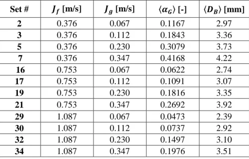
Of the 42 turbulent flow conditions explored in the original test matrix of Liu and Bankoff, we have selected 12 representative experimental sets to test and assess the closures, as specified in Table 1. As can be seen in table 1, these 12 cases almost span the full breadth of the experimental range.
Table 1. Selected sets from the Liu and Bankoff experimental database
Set # [m/s] [m/s] 〈 〉 [-] 〈 〉 [mm] 2 0.376 0.067 0.1167 2.97 3 0.376 0.112 0.1843 3.36 5 0.376 0.230 0.3079 3.73 7 0.376 0.347 0.4168 4.22 16 0.753 0.067 0.0622 2.74 17 0.753 0.112 0.1091 3.07 19 0.753 0.230 0.1816 3.35 21 0.753 0.347 0.2692 3.92 29 1.087 0.067 0.0473 2.39 30 1.087 0.112 0.0737 2.92 32 1.087 0.230 0.1497 3.10 34 1.087 0.347 0.1976 3.51
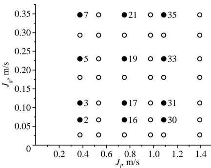
Figure 1. Liu and Bankoff experimental range. Shaded circles denote cases examined and simulated in this work.
2. Physical modeling
As briefly discussed in the introduction, in the two-fluid approach each phase is described by a balance of mass, momentum and energy, and interphase transfers are modeled through closure relations. Here, the flow being adiabatic, the energy equation is not taken into account, and there is no transfer term in the mass balance. The implementation in the two CFD codes is described in the following sections, where the reader is referred to the specific literature for well assessed formulations.
2.1. NEPTUNE_CFD
Interfacial momentum exchange
The standard model for the interfacial momentum exchange term implemented in NEPTUNE_CFD is decomposed into a sum of five contributions: drag, virtual mass, lift, wall forces, and a model for turbulent dispersion referred to as the Generalized Turbulent Dispersion Model of (Laviéville, 2015).
(Ishii and Zuber, 1979) express the drag coefficient for small spherical bubbles as
= 1 + 0.1 .
where is the bubble Reynolds number = !"# ‖% − %"‖/ )". In (Zuber, 1964), the virtual mass coefficient *+ is expressed as
*+ = 121 + 2-1 − -0.2 0.4 0.6 0.8 1.0 1.2 1.4 0.05 0.10 0.15 0.20 0.25 0.30 0.35 0 2 3 5 7 16 17 19 21 30 31 33 35 J g , m /s Jl, m/s
The lift force is expressed by the model in (Tomiyama et al., 2002), where the lift coefficient . depends on the bubble Eötvös number /0.
The wall force accounts for the experimental observation that the void fraction is zero at the walls. Three main models are available in the literature. Denoting by y the distance to the wall, these models express the wall force proportionally to 1 13 , with different values of exponent p: p = 1 for Antal 2
et al (1991), p= 2 for Tomiyama et al. (2002), p = 1.7 for Frank et al. (2008). Tomiyama’s model was selected in NEPTUNE_CFD.
The turbulent dispersion force is accounted for with the Generalized Turbulent Dispersion Force model developed in (Laviéville et al., 2015). This force represents the turbulent part of previous ones (mainly Drag and Virtual Mass effects) and is formally derived by comparison between Lagrangian and Eulerian description of bubbles motion. It is proportional to the void fraction gradient, and results in the migration of bubbles from high to low void fraction regions
4.→67 = − 7 !"8"∇-
where 8" is the turbulent kinetic energy of the liquid phase. The turbulent dispersion coefficient 7 is given by
7 = :〈; 〉<"= − 1>? + @1 + @A
A+ 〈 *+〉 ? + @ A
1 + @A
with 〈; 〉, <"= , ?, @A defined as follows:
<"= =3 2 D8E""F1 + G HA 8"I "/ , D = 0.09, G = 2.7 〈; 〉 =18 # ‖% − %6 "‖ @A =<" = <"N <"N = 〈; 〉O"P!! "+ *+Q ? = P!! + !"+ !" *+ " *+Q
Turbulence and Turbulent Reverse Coupling
Turbulence in the liquid phase is accounted for through a second-order, RS− E model (Mimouni et al, 2009). Two-phase extra contributions are included in the Reynolds Stress Tensor ",RS and Turbulent dissipation T" equations, corresponding to bubble-induced turbulence, writing as:
U:-"!" ",RS> UV + ⋯ = ⋯ + 23 - ;" G HA XRS+ 3:1 − G >HA,RHA,S U:-"!"E"> UV + ⋯ = ⋯ + ;" HA min :- , 0.5>< With ;" = 34 !# % G = 2 3" ⁄ % = ‖% − %"‖ < = _`a bF#E "I " c , 1 d 8" E"e d = 1.83 8" = 1 2 ",""+ ", + ",cc 2.2 STAR-CCM+
The closure set adopted in STAR-CCM+ for this assessment leverages the experimentally measured bubble diameters in order to eliminate this unknown, and focuses on the interfacial forces. Earlier sensitivity studies have demonstrated that the use of a constant bubble diameter size is equivalent, for the current Liu and Bankoff conditions, to adopting radially varying dimension; in the calculation the Sauter mean diameter is therefore computed by averaging the experimental measurements. The drag coefficient (CD) is modeled using the formulation by Tomiyama et al (1998b), assuming slight
contamination of surfactants. A constant lift coefficient (CL0) equal to 0.025 is prescribed for the
entire domain, and is damped to zero in the near-wall region using the Shaver and Podowski correction (2015): . = f g h g i 0,kj < " . P3 mkj− 1n − 2 mkjo− 1n c Q ,"≤kjo≤ 1 . , 1 < kjo
where CL0 is the nominal lift coefficient (0.025), db is the bubble diameter, and y is the wall-normal
distance. The applicability of the lift coefficient value for small spherical bubbles was demonstrated in Baglietto (2013) and builds on the extensive work of Podowski (as discussed in Shaver and Podowski, 2015). Turbulent dispersion is modeled using the formulation by Burns et al (2004) with
σ
TD = 1.0.The wall-lubrication force 4.→6q is modeled using an expression derived through an analytical regularization of turbulent dispersion in the near-wall region to account for the decreasing cross-sectional area of the bubbles. This formulation, recently advanced by Lubchenko et al. (2018), assumes a quadratic dependence of gas volume fraction on wall-normal distance:
4.→6q =c m1 +"Orr nvDwxstku -"j y
zOj k Oj
Here, CD is the drag coefficient, α is the gas volume fraction, UR is the relative velocity between
phases, and µt is the turbulent viscosity, which was calculated using the standard k-ε model
In contrast to previous methods, which interpreted the lubrication force as a physical force pushing bubbles away from the wall, this work brings forward a renewed understanding, where the gas fraction distribution is a direct consequence of a reduction in cross-sectional area of the bubbles, by virtue of their shape, which is assumed as spherical. The formulation is therefore very general and does not require the use of tunable coefficients.
2.3 Summary
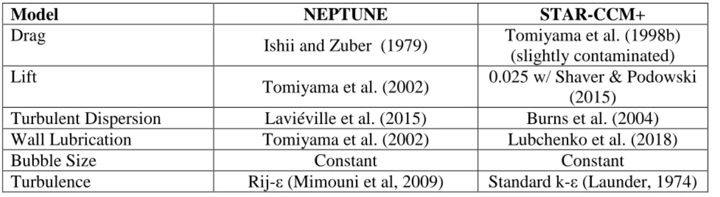
Table 2 summarizes the prescribed interfacial forces and turbulence models utilized in NEPTUNE_CFD and STAR-CCM+ simulations.
Table 2. Interfacial Closures Models in the CFD simulations
Model NEPTUNE STAR-CCM+
Drag
Ishii and Zuber (1979) Tomiyama et al. (1998b) (slightly contaminated) Lift
Tomiyama et al. (2002) 0.025 w/ Shaver & Podowski (2015)
Turbulent Dispersion Laviéville et al. (2015) Burns et al. (2004) Wall Lubrication Tomiyama et al. (2002) Lubchenko et al. (2018)
Bubble Size Constant Constant
Turbulence Rij-ε (Mimouni et al, 2009) Standard k-ε (Launder, 1974)
3. Numerical set-up
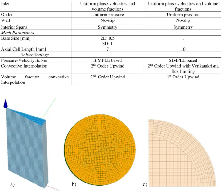
The flow being axisymmetric, calculations with the NEPTUNE_CFD code are performed both on 2D-axisymmetric and 3D domains. The 2D computational domain is a cylindrical sector with internal angle 11° and symmetry boundary conditions imposed on both lateral faces. The 3D domain is the whole cylindrical pipe with radius 19 mm and height 2.8m (Figure 2, a and b). Hexaedral meshes are used in 3D. The meshes are built with the SALOME platform, developed by CEA and EDF. The boundary conditions are imposed as summarized in table 3.
For calculations with STAR-CCM+, a quarter-pipe geometry has been simulated for the twelve cases selected from the Liu and Bankoff experimental database. The mesh is an hexa-dominant mesh with boundary fitted meshes in the near wall region, where prismatic cells connect the boundary fitted region to the core hexahedral mesh (Figure 1, c). The mesh is constructed in STAR-CCM+ using the automated Trimm and Prism layer meshers, and is representative of industrial meshes adopted for fuel assembly simulations (Brewster, 2015).
Table 3 – Summary of boundary conditions and numerical options used by each team
NEPTUNE STAR-CCM+
Computational Geometry
Length [m] 2.800 1.600
Radius [m] 0.019 0.019
Inlet Uniform phase-velocities and volume fractions
Uniform phase-velocities and volume fractions
Outlet Uniform pressure Uniform pressure
Wall No-slip No-slip
Interior Spans Symmetry Symmetry
Mesh Parameters
Base Size [mm] 2D: 0.5
3D: 1
1
Axial Cell Length [mm] 7 10
Solver Settings
Pressure-Velocity Solver SIMPLE based SIMPLE based
Convective Interpolation 2nd Order Upwind 2nd Order Upwind with Venkatakrisna
flux limiting Volume fraction convective
Interpolation
2nd Order Upwind 1st Order Upwind
Figure 2. Computational Meshes: a): NEPTUNE CFD 2D axisymmetric mesh – b) top view of the NEPTUNE_CFD 3D mesh – c) STAR-CCM+ quarter symmetry 3D mesh
4. Results
The predicted mean profiles of liquid and gas velocities and void fraction are presented in comparison to the experimental measurements for the 12 selected cases from the Liu and Bankoff experimental databases. The comparison for both NEPTUNE_CFD and STAR-CCM+ simulations provides a qualitative understanding of results.
4.1. Liquid velocity profiles
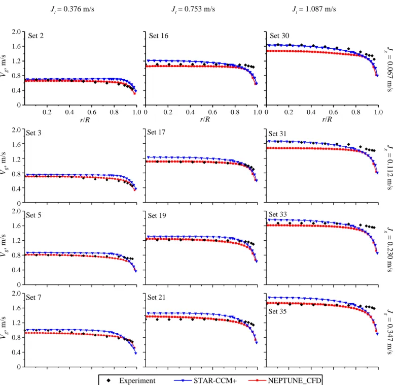
Figure 3. Numerical and experimental liquid velocity profiles for the twelve selected test cases
Jl = 0.376 m/s Jl = 0.753 m/s Jl = 1.087 m/s 0.2 0.4 0.6 0.8 1.0 0.4 0.8 1.2 1.6 0 r/R Vl , m /s Set 2 0.2 0.4 0.6 0.8 1.0 0 Set 16 r/R 0.2 0.4 0.6 0.8 1.0 0 r/R Set 30 J g = 0 .0 6 7 m /s 0.4 0.8 1.2 1.6 0 Vl , m /s
Set 3 Set 17 Set 31
J g = 0 .1 1 2 m /s 0.4 0.8 1.2 1.6 0 Vl , m /s Set 5 Set 19 Set 33 gJ = 0 .2 3 0 m /s 0.4 0.8 1.2 1.6 2.0 0 Vl , m /s
Set 7 Set 21 Set 35
J g = 0 .3 4 7 m /s
4.2. Gas velocity profiles
Figure 4. Numerical and experimental gas velocity profiles for the twelve selected test cases
4.3.Void fraction profiles
Jl = 0.376 m/s Jl = 0.753 m/s Jl = 1.087 m/s 0.2 0.4 0.6 0.8 1.0 0.4 0.8 1.2 1.6 2.0 0 r/R Set 2 Vg , m /s 0.2 0.4 0.6 0.8 1.0 0 r/R Set 16 0.2 0.4 0.6 0.8 1.0 0 r/R Set 30 J g = 0 .0 6 7 m /s 0.4 0.8 1.2 1.6 2.0 0 Set 3 Vg , m /s Set 17 Set 31 J g = 0 .1 1 2 m /s 0.4 0.8 1.2 1.6 2.0 0 Set 5 Vg , m /s Set 19 Set 33 J g = 0 .2 3 0 m /s 0.4 0.8 1.2 1.6 2.0 0 Set 7 Vg , m /s Set 21 Set 35 gJ = 0 .3 4 7 m /s
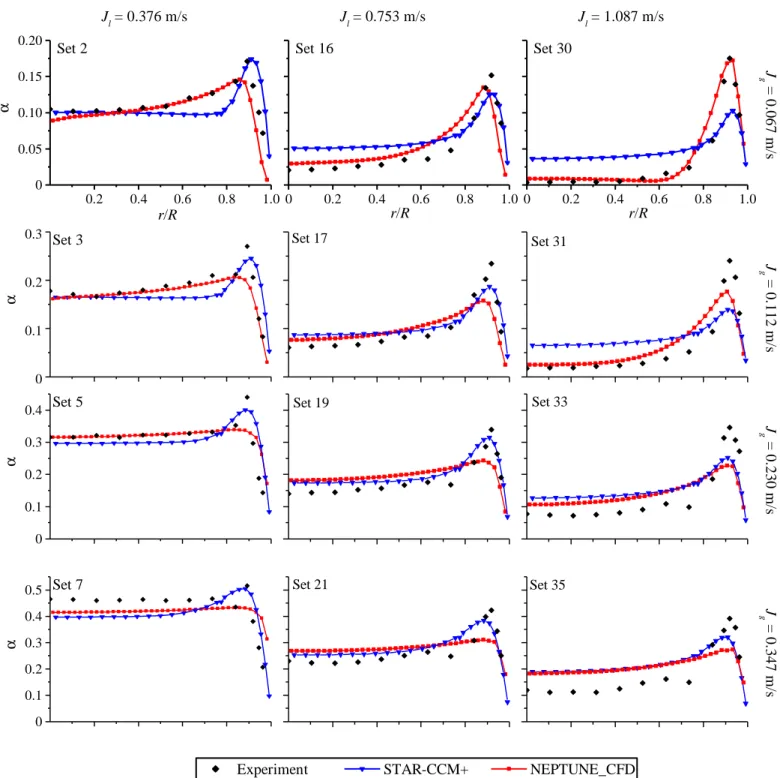
Figure 5. Numerical and experimental void fraction profiles for the twelve selected test cases
5. Discussion
Radial distributions for the liquid velocity profiles are summarized in Figure 3. Both codes provide high quality predictions across the entire test matrix. The numerical predictions are very close to
Jl = 0.376 m/s Jl = 0.753 m/s Jl = 1.087 m/s 0.2 0.4 0.6 0.8 1.0 0.05 0.10 0.15 0.20 0 r/R α Set 2 0.2 0.4 0.6 0.8 1.0 0 r/R Set 16 0.2 0.4 0.6 0.8 1.0 0 r/R Set 30 J g = 0 .0 6 7 m /s 0.1 0.2 0.3 0 Set 3 α Set 17 Set 31 J g = 0 .1 1 2 m /s 0.1 0.2 0.3 0.4 0 Set 5 α Set 19 Set 33 J g = 0 .2 3 0 m /s 0.1 0.2 0.3 0.4 0.5 0 Set 7 α Set 21 Set 35 J g = 0 .3 4 7 m /s
each other for low and moderate liquid superficial velocities (Jf=0.376 and 0.753 m/s), whereas a
somewhat larger discrepancy between the predictions of the two codes can be observed for the highest value of Jf. Both codes predict a flat profile for set 7 (low Jf high Jg), which derives from the
void fraction underprediction for this case, and the consequent underestimation of the buoyancy accelerating the bulk region of the flow.
Similar observations can be made for the gas velocity prediction, shown in Figure 4. Again, the numerical predictions are close to each other for low and moderate liquid superficial velocities (Jf=0.376 and 0.753 m/s), whereas a somewhat larger discrepancy between the predictions of the two
codes can be observed for the highest value of Jf. The higher velocities predicted by STAR-CCM+
would indicate that the drag force is underpredicted by the slightly contaminated Tomiyama correlation and will be discussed in more detail in the following sections. Particularly challenging conditions appears to be the high liquid and low gas velocity (sets 30, 31) where NEPTUNE_CFD provides particularly fitting void fraction and liquid velocity distributions, while STAR-CCM+ better predicts the gas velocities.
Looking at the void fraction distributions in Figure 5, both sets of closures deliver acceptable predictions for the whole experimental database. For the low liquid flow cases (Sets 2, 3, 5,16) the NEPTUNE_CFD results appear to produce a qualitatively better agreement with the bulk void distribution, thanks to the advanced turbulent dispersion formulation. On the contrary, the STAR-CCM+ results cannot closely match the bulk void distributions where the lack of a bubble induced turbulence mechanism leads to a clear underprediction of the dispersion.
5.1. Lateral redistribution forces:
One of the major challenges in predicting bubbly flows in CFD is related to the still incomplete understanding of the lateral redistribution forces.
For bubbly flow regimes, the lateral distribution of the gas phase is controlled by lift, turbulent dispersion, and wall forces. This is illustrated by recent work by Marfaing et al (2016, 2017), who investigate low Reynolds number bubbly flows in pipes, and exhibit an analytical expression (Bubble Force Balance Formula - BFBF) for the radial void fraction profile. This BFBF profile is compared to experimental data and Direct Numerical Simulations from the literature, as discussed in the next section.
For the upward flow configuration of interest, the small quasi-spherical bubbles are pushed towards the wall by the lift force, resulting in a characteristic wall-peaked void fraction distribution. Turbulent dispersion acts to flatten the void fraction distribution, while a wall force is commonly adopted to control the steep near wall void fraction gradient and is discussed later.
In the absence of appropriate general closures for bubbly flow, the only available formulation has been derived by Tomiyama (2002) for a single rising bubble in a uniform shear rate laminar flow. In general bubbly flow conditions the interaction of bubbles and wakes strongly reduces the effective lift force; testing (Baglietto and Christon, 2013, Shaver and Podowski 2015) has indicated that the actual lift force differs approximately by an order of magnitude from the single bubble values proposed by Tomiyama. A numerical evaluation of the effective lift force from the DNS data for bubbly flow from Bolotnov (2013) shows an effective lift coefficient CL = 0.015, in contrast with the
The NEPTUNE_CFD and CASL approaches take different directions in approaching this challenge: on the one side the NEPTUNE_CFD closures start from the single bubble Tomiyama lift closure and account for the bubble interaction through a novel turbulent dispersion closure proposed by Laviéville (2015); on the other the STAR-CCM+ closure leverages a constant lift coefficient based on previous optimizations and couples it with the classic turbulent dispersion by Burns (2004), which is directly derived to account for the unsteady drag component in the lateral direction. Neither of the two approaches is superior, and a more general lift closure formulation is required, which should be able to include the effects of void fraction and liquid flow turbulence in addition to the classic Eötvös number proposed by Tomiyama. If we look in detail at the void fraction distributions in Figure 3, for the low liquid flow cases (Sets 2, 3, 5,16) the NEPTUNE_CFD results appear to produce a qualitatively better agreement with the bulk void distribution, thanks to the advanced turbulent dispersion formulation. On the contrary, the STAR-CCM+ results cannot closely match the bulk void distributions where the lack of a bubble induced turbulence mechanism leads to a clear underprediction of the dispersion.
To understand the importance of the lateral redistribution forces it is useful to underline how the void fraction distribution in vertical upflow also plays a dominant contribution in the liquid velocity distribution. Large void peaks near the wall with lower void fraction in the bulk cause a large buoyancy effect near the wall that leads to practically flat velocity profiles. Larger void fraction in the bulk region instead mean larger contribution of buoyancy away from the wall and lead to more parabolic profiles. A particularly useful example is given by Set 7, where the CFD underpredicts the void fraction in the center, therefore overpredicting the buoyancy near the wall, producing flatter velocity profiles than measured.
5.2. Near-wall hydrodynamic effects
The near wall void fraction distribution, as just discussed, plays an important role in the liquid velocity distribution, and its accurate prediction is especially important in the framework of future application to DNB. Three main models have been developed to describe the near wall void fraction distribution through the prescription of a force to push the gas away from the wall. Denoting by y the distance to the wall, these models express the wall force proportionally to 1 13 , with different values 2
of exponent p: p = 1 for Antal et al (1991), p= 2 for Tomiyama et al. (2002), p = 1.7 for Frank et al. (2008).
In recent work, Marfaing et al (2017) compare and assess these three wall force models. Basing on the analytical work developed in (Marfaing et al, 2016), they observe that the choice of the model impacts the rate with which the analytical void fraction profile goes to zero at the wall. Using experimental measurements (Nakoryakov et al, 1996; Hosokawa and Tomiyama, 2013) and DNS simulations (Lu et al, 2006) of low Reynolds bubbly flows from the literature, it is found that an Antal-like model, in 13 , yields the best agreement. 1
All of these models result in wall forces that propagate a few bubble diameters away from the wall.
Lubchenko (2017), has recently re-evaluated the fundamental assumption of the Antal lubrication, noting how both experimental measurements (Hassan, 2014) and DNS data (Lu and Tryggvasson, 2013) indicate that bubbles directly contact the wall, leading to the conclusion that no macroscopic
force exists to push the bubbles away from the wall. Rather, the two-fluid averaging of near wall bubbles leads to a parabolic void fraction profile, as schematically represented in Figure 6.
(a) (b) (c)
Figure 6. (a) Side view of bubbles sliding along a wall. (b) Front view of cross-sections of bubbles. (c) Cross-section of gas phase as function of distance from the wall [From Lubchenko, 2017].
Starting from this fundamental postulation the void fraction distribution can be computed analytically. Finally an artificial lubrication force can be derived as a near wall regularization of the turbulence dispersion that allows to recover the correct analytical void profile. The new wall lubrication was presented in Section 2.2, and does not require the use of limiters and tunable coefficients, greatly improving the general applicability and ease of use of the model. The obtained expression is in 13 , in agreement with the conclusions of (Marfaing et al, 2017). 1
5.3. Influence of turbulence modeling:
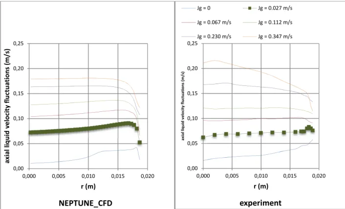
In their experiments, Liu and Bankoff systematically record the liquid velocity fluctuations, defined as the standard deviation of the liquid velocity. Since a Reynolds-stress model is used in the NEPTUNE_CFD code, we can make a direct comparison of the (square root of the) turbulent stresses with the measurements. The results are displayed in Figures 7 to 10 below. Figure 7 shows the axial velocity fluctuations for Jf = 0.376 m/s, with increasing values of the gas superficial velocity Jg. In order to enrich the physical discussion, we add the results for Jg = 0 and 0.027 m/s.
On a quantitative basis, the calculations are seen to be in reasonable agreement with the measurements. On a qualitative basis, we can see that, for low liquid flow (Jf = 0.376 m/s), the fluctuations increase with increasing gas flow: bubbles generate liquid agitation. This qualitative trend is correctly reproduced by the simulations, which makes use of a bubble-induced fluctuation model. For comparison, we also run computations with NEPTUNE_CFD without the bubble-induced agitation model. The results are displayed in Figure 8. They reveal that a bubble-induced agitation model is necessary to reproduce the increase in fluctuations with increasing gas flow.
1 2 3 1 2 3 0.0 0.5 1.0 A , m m 2 y/D, [−]
Fig 7. Axial liquid velocity fluctuations for Jf = 0.376 m/s with increasing values of Jg. Left: NEPTUNE_CFD calculations. Right: experimental measurements.
Fig 8. Axial liquid velocity fluctuations for Jf = 0.376 m/s, calculated with NEPTUNE_CFD. Left: computations with the bubble-induced agitation model. Right: without the bubble-induced agitation model.
0,00 0,05 0,10 0,15 0,20 0,25 0,000 0,005 0,010 0,015 0,020 ax ial l iq u id v e lo ci ty f lu ct u at io n s (m /s ) r (m) NEPTUNE_CFD 0,00 0,05 0,10 0,15 0,20 0,25 0,000 0,005 0,010 0,015 0,020 a x ia l li q u id v e lo ci ty f lu ct u a ti o n s (m /s ) r (m) experiment Jg = 0.067 m/s Jg = 0.112 m/s Jg = 0.230 m/s Jg = 0.347 m/s 0,00 0,05 0,10 0,15 0,20 0,25 0,000 0,005 0,010 0,015 0,020 ax ial l iq u id v e lo ci ty f lu ct u at io n s (m /s ) r (m)
NEPTUNE_CFD with bubble-induced agitation 0,00 0,05 0,10 0,15 0,20 0,25 0,000 0,005 0,010 0,015 0,020 ax ial l iq u id v e lo ci ty f lu ct u at io n s (m /s ) r (m)
NEPTUNE_CFD calculations without bubble agitation model
Jg = 0 Jg = 0.027 m/s Jg = 0.067 m/s Jg = 0.112 m/s Jg = 0.230 m/s Jg = 0.347 m/s
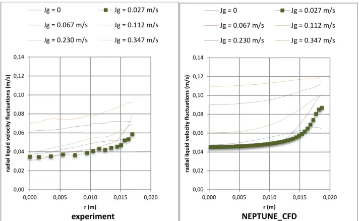
A different behavior is observed for higher liquid flows. This is illustrated in Figure 9 for Jf = 1.087 m/s, which displays the liquid radial velocity fluctuations. On a quantitative basis, the calculations are seen to be in reasonable agreement with the measurements. On a qualitative basis, Liu and Bankoff notice that, in the center of the pipe, the liquid fluctuations for Jg = 0.027 and 0.067 m/s are lower than for the single-phase flow, a phenomenon which they refer to as turbulence suppression. The fluctuations then increase when the gas flow is further increased. This effect means that for high liquid flow conditions, the introduction of bubbles not only increases the production of turbulence, but also its dissipation. For high Jf and low Jg, the increase in dissipation is higher than the increase in production. This qualitative trend is reproduced by the simulations.
Again, we also run computations with NEPTUNE_CFD without the bubble-induced agitation model. The results are displayed in Figure 10. As in the low flow case, the bubble-induced agitation model is necessary to reproduce the variations in fluctuations for increasing gas flow.
Fig 9. Radial liquid velocity fluctuations for Jf = 1.087 m/s with increasing values of Jg. Left: NEPTUNE_CFD calculations. Right: experimental measurements.
0,00 0,02 0,04 0,06 0,08 0,10 0,12 0,14 0,000 0,005 0,010 0,015 0,020 ra d ia l li q u id v e lo ci ty f lu ct u a ti o n s (m /s ) r (m) experiment Jg = 0 Jg = 0.027 m/s Jg = 0.067 m/s Jg = 0.112 m/s Jg = 0.230 m/s Jg = 0.347 m/s 0,00 0,02 0,04 0,06 0,08 0,10 0,12 0,14 0,000 0,005 0,010 0,015 0,020 ra d ia l li q u id v e lo ci ty f lu ct u a ti o n s (m /s ) r (m) NEPTUNE_CFD Jg = 0 Jg = 0.027 m/s Jg = 0.067 m/s Jg = 0.112 m/s Jg = 0.230 m/s Jg = 0.347 m/s
Fig 10. Radial liquid velocity fluctuations for Jf = 1.087 m/s, calculated with NEPTUNE_CFD. Left: computations with the bubble-induced agitation model. Right: without the bubble-induced agitation model.
5.4. Other hydrodynamic effects
Figure 5 presented the comparison of the gas velocity distributions, and evidenced that for the low liquid flux cases (sets 2, 3, 5), the STAR-CCM+ results predicted consistently higher gas velocities in comparison to the experiment and to the NEPTUNE predictions. In order to better understand this difference, terminal velocities for single bubbles predicted by Ishii-Zuber and Tomiyama drag models are shown in Fig 11.
0,00 0,02 0,04 0,06 0,08 0,10 0,12 0,14 0,000 0,005 0,010 0,015 0,020 ra d ia l li q u id v e lo ci ty f lu ct u a ti o n s (m /s ) r (m)
NEPTUNE_CFD with bubble agitation model Jg = 0 Jg = 0.027 m/s Jg = 0.067 m/s Jg = 0.112 m/s Jg = 0.230 m/s Jg = 0.347 m/s 0,00 0,02 0,04 0,06 0,08 0,10 0,12 0,14 0,000 0,005 0,010 0,015 0,020 ra d ia l li q u id v e lo ci ty f lu ct u a ti o n s (m /s ) r (m)
NEPTUNE_CFD calculations without bubble agitation model
Jg = 0 Jg = 0.027 m/s
Jg = 0.067 m/s Jg = 0.112 m/s
Figure 11. Impact of bubble diameter and drag model on bubble terminal rise velocity
Ishii-Zuber and Tomiyama models predict very similar terminal velocities, where the difference for small diameters is due to contamination. High contamination reduced the mobility of the surface, therefore increasing the drag and reducing the relative velocity. This comparison indicated that the assumption of slight contamination, which is expected to be applicable to reactor coolant, is not necessarily appropriate for the Liu and Bankoff experiments, where the contaminated Tomiyama formulation would improve the results consistently with the Ishii-Zuber formulation.
6. Uncertainty quantification
Quantifying parametric uncertainties and propagating them through relevant models is becoming an important aspect of nuclear safety studies, and we consider the quantification and propagation of such uncertainties in the particular context of interphase momentum closures in this section. First, we perform a series of non-intrusive analyses of bubbly flow in STARCCM+ using Dakota and then conduct a comprehensive Bayesian analysis of the closures. The intent of these studies is to illustrate the kinds of methods that are likely to help in the process of better characterizing the closures and their mutual interactions. Given that there are closures of numerous processes in the CFD modeling of turbulent multiphase flows, and that the development of such closures does not always take into account all of the other closures, these methods serve to comprehensively analyze interactions between the closures in an a posteriori fashion and can provide insight into unforeseen interactions. As such, we expect that these methods will have an increasingly important role to play in making the modeling of turbulent multiphase flows robust.
6.1 Non-instrusive analysis of bubbly flow in STARCCM+ using Dakota
The Dakota software toolkit (Adams et al., 2016) provides a range of capabilities for exploration and design of computational simulations. It contains algorithms for optimization, uncertainty quantification, sensitivity analysis, and model calibration. A comprehensive Bayesian analysis of an example multiphase flow as simulated by STAR-CCM+ is thought to be not computationally feasible presently. For this reason, in this work, Dakota's sampling, polynomial chaos, deterministic
0
1
2
3
4
5
6
0.0
0.1
0.2
0.3
0.4
V
r,
m
/s
D
b, mm
Ishii-Zuber
Tomiyama (clean)
Tomiyama (slightly cont.)
Tomiyama (contaminated)
and void fraction profiles predicted by STAR-CCM+ to three model parameters, then to identify model parameter values to match the Liu-Bankoff test case observations, and finally to assess the optimality of this calibration. Here we choose the Liu-Bankoff test case that corresponds to a liquid superficial velocity Jf of 1.087 m/s and a gas superficial velocity Jg of 0.067 m/s.
6.1.1 Sampling Study
We choose lift, drag, and wall lubrication closures for this study. In order to determine the sensitivity of the velocity and void fraction profiles to the three model parameters, we first use Dakota's Monte Carlo sampling method to run the model at 300 randomized locations in parameter space. A Latin Hypercube (LHS) design, the Dakota default, is used to stratify the samples. LHS designs exhibit space-filling properties superior to purely random designs. The radial profiles of void fraction and fluid velocity at z/D of 36 as represented in the STAR-CCM+ solution of the Liu-Bankoff experiment considered are identified as the quantities of interest. Here, z is the axial location (flow direction) and D refers to the diameter of the pipe in the Liu-Bankoff setup. Information about the radial profiles is conveyed to Dakota by a shell script. Further, a “recover'' failure capture strategy was used, wherein if the STAR-CCM+ solution at a given sampling point was found to be too far from the experimental measurements (in the experimental measurement space), that region of the parameter space is flagged as uninteresting from the point of view of the sampling study and the associated correlation analysis. The tasks of detecting failures and running STAR-CCM+ are handled by the same shell script.
For this sampling study, the three parameters considered are the lift coefficient CL in the Tomiyama
form of the parameterization of lift force (see Sec. 2.1; -0.25 < CL < 0.25) and Cwl1 and Cwl2, the two
coefficients used in the Antal (1991) form of the parameterization of wall lubrication force (-0.03 < Ccwl1 < 0.00; 0.0 < Ccwl2 < 0.10; see 5.2, however). The coefficient of drag is modeled using the
formulation by Tomiyama (1998b), assuming slight contamination of surfactants, and was therefore not a parameter in the study.
Figure 12. Fluid velocity profiles (left) and void fraction profiles (right) from the sampling study along with the experimental measurements of Liu-Bankoff, 1993.
Results from the sampling study are summarized in terms of the fluid velocity profiles (left) and void fraction profiles (right) in Fig. 12. Also shown in symbols are the experimental measurements of Liu-Bankoff, 1993. From this figure, it is clear that the void fraction profile has a much stronger dependence on the lift and wall-lubrication coefficients than the fluid velocity profile. This greater
sensitivity of void fraction may be understood as arising from the strong nonlinearity of the two-fluid model, and as we will see next. Furthermore, changes to wall-lubrication are seen to cause changes more globally than just the wall region where the parameterization was intended to be active. Again, this feature will become clearer in the correlation and sensitivity analyses presented next.
Of the 300 sample parameter vectors considered, a handful did not produce converged results, and a few others produced converged results (fluid velocity and void fraction profiles) very far from the measurements (see Fig. 12) and were eliminated from Fig. 13. In this figure, it is also seen that the highly nonlinear nature of the two-fluid model leads to a much greater sensitivity of the void fraction behavior as compared to the fluid-velocity profile.
Finally, we note that a regular grid based sampling study was also conducted and produced similar results. Dakota's sampling method computes a number of quantities that can be helpful in assessing sensitivity. In particular, partial Pearson's and partial Spearman's correlation coefficients, also referred to as partial correlations and partial rank correlations, indicate linear correlation between variables and responses. They are termed 'partial' (rather than simple) because the effects of other variables have been removed. Pearson's correlations are computed using the values of the variables and responses directly, while Spearman's correlations use the ranks of the values instead, making them a test of monotonicity. Both kinds of coefficient can take on values between 1 and +1, with -1 indicating a perfect inverse linear relationship, +-1 indicating a perfect direct linear relationship, and values in between indicating weaker relationships.
Figure 13: Correlation of fluid velocity profile (left) and void fraction profile with respect to lift and wall lubrication parameters. Partial (simple) correlations are shown in solid lines and partial rank correlations are shown in dashed lines.
The larger difference between the simple and rank correlations for the void fraction profile indicates a higher degree of nonlinearity in the relationship between the void fraction profile and the input parameters.
6.1.2 Polynomial Chaos Expansion Based Sensitivity
Variance-based decomposition (VBD) is another form of sensitivity analysis in which the variance of a response is apportioned to contributions made by each variable. Dakota reports the contributions of variables as main, interaction, and total effects, also known as Sobol indices. The main effect of a variable indicates the strength of its individual contribution to response variance, while interaction
effect is the sum of its main effect and all interaction effects in which it participates. The main and interaction effects of all variables sum to unity (not so for total effects), and each one may be interpreted as a fractional contribution to response variance. The main effect of variable aR on response { is defined as |R = }`~•R€/•~R:{|aR>ƒ / }`~:{>, where / and }`~ denote the expectation value and variance respectively, and a~R indicates the set of all parameters except aR. Similarly, the total effect of variable aR on response { is defined as |7R = /•~R:}`~•R:{|a~R>> / }`~:{>, the interaction effect of variables aR and aS on { as |RS = }`~•RS„/•~RS {…aR, aS † / }`~:{> − |R− |S, and so on.
6.1.3 Global Sensitivity
The total effects of each model parameter across the velocity and void fraction profiles are plotted in Fig. 14. The lift coefficient, fairly consistently, has the greatest effect on both responses, while the two wall lubrication coefficients also have sizable influence at certain radii. It can be concluded from the results (see Fig. 15), that sensitivity of both fluid velocity and void fraction profiles is dominantly on the lift coefficient. From Fig. 16, further it is evidencedthat the sensitivity to wall lubrication coefficients occurs primarily through their interactions with the lift coefficient in both the fluid velocity and void fraction profiles. While a greater sensitivity of the void fraction profile on the mutual interaction between the wall lubrication coefficients is expected and seen in Fig. 15, it is interesting to observe that this sensitivity is not confined to the region near the wall (normalized radial position of 1) and is indeed bigger in the interior region than in the region near the wall.
The total, main, and interaction effects and the correlation coefficients presented, indicate that all three parameters are significant in their effect on the radial profiles of fluid velocity and void fraction and should therefore be considered in calibration studies.
Figure 14. The fluid velocity and void fraction profiles are both seen to be dominantly sensitive to the value of the lift coefficient. Their sensitivity to the wall lubrication coefficients is however seen to be significant with this sensitivity being greater for the void fraction profile.
6.1.4 Calibration Study
Following the sampling-based correlations and the PCE-based sensitivities in the previous sections, we further leveraged Dakota's trust-region method for nonlinear least squares, ‘nl2sol’, to identify optimal values for the lift and wall lubrication coefficients. This method is a gradient-based local
optimizer that tunes model parameters to minimize the sum-squared error between model predictions, which are provided to Dakota by the user's simulation, and experimental observations.
Figure 15. In terms of their main effect on fluid velocity and void fraction profiles, the influence of lift coefficient is out-sized, except for the effect on the void fraction profile in the region near the wall.
Figure 17 shows the fluid velocity profile in the left panel and the void fraction profile in the right panel at the optimal combination of parameter values (indicated on top) resulting from the calibration study along with the experimental measurements of Liu-Bankoff (1993). In the two plots in Fig. 17, the sum of squared-error and the sum of absolute-error are shown in the legend as well. A first observation is that the calibration process does not capture the peak in the void fraction profile in the region near the wall. This behavior could derive from the optimization method ‘nl2sol’ used in Dakota, which being based on local gradients can depend on the starting assumption. Unfortunately, attempts at using a global calibration method (such as those based on an evolutionary algorithm) ran into excessive run times. Further, in the work we attempted to optimize a set of parameters based on the model representation of the fluid velocity profile and the void fraction profile. Given the different nature of these two profiles, this optimization problem should be properly handled as multi-objective optimization problem; the present study is, however, based on least-squares.
Figure 16. Although the main effect of the lift coefficient is large compared to that of the wall lubrication coefficients, the interaction of these latter coefficients with the lift coefficient and between themselves is seen to have a large effect on both profiles.
was further evaluated. It is known that adopting an L2 (or L∞) norm leads to recovering more generic
representations whereas using an L1 norm leads to recovering less-generic and sparse representations,
and it is possible that the restricted parameterizations (lack of full physics) that we are currently using leads to a better representation of the experimental data in a less-generic sense. For this reason, we attempt an L1 regularization, and the results are shown in Fig. 18. With the L1 error norm, a better fit
of the void fraction profile (right) is indeed realized in the sense of capturing the peak near the wall. Simultaneously, however, while a better fit of the fluid velocity profile is realized away from the wall, larger deviations are seen in the region near the wall.
Figure 17. Fluid velocity profile (left) and void fraction profile (right) resulting from the calibration study along with the experimental measurements of Liu-Bankoff, 1993. The peak in the void fraction adjacent to the wall is not captured by the calibration.
Figure 18. On using an L1 norm for the calibration study, a better fit of the void fraction profile (right) is
realized in terms of capturing the peak near the wall. Simultaneously, while a better fit of the fluid velocity profile is realized away from the wall, larger deviations are seen in the region near the wall.
6.2 Bayesian Analysis
Attempts at leveraging global techniques, such as those based on evolutionary algorithms in Dakota coupled to STAR-CCM+ ran into long execution time issues, suggesting its impracticability. Therefore, in order to evaluate the use of global techniques in analyzing multiphase closures, we consider fully-developed flow in a vertical cylindrical pipe and develop a numerical model for it. For details see Nadiga et al. (2016), and Nadiga and Baglietto (2017).
Figure 19. Posterior envelopes of fluid-velocity, void-fraction and turbulent velocity fluctuation profiles in Liu Bankoff test case with Jf=1.087 m/s and Jg=0.067 m/s.
An extensive Bayesian calibration study was performed, adopting the same lift, drag, wall-lubrication, and turbulence (standard k-ε) closures previously discussed. Figure 19 shows the posterior predictive envelope for the quantities of interest (radial profiles of fluid-velocity, void-fraction and turbulent fluid-velocity fluctuations) for the flow conditions that had been characterized in the STARCCM+-Dakota study. That is, a Markov Chain Monte Carlo (MCMC) sampler was constructed and used in conjunction with the multiphase flow solver and the measurements of Liu and Bankoff, to obtain the posterior distribution of all the closure-parameters considered. Then the joint distribution of parameters was propagated through the flow solver to obtain the envelope of the quantities of interest. In the calibration process, only the fluid-velocity and void-fraction measurements of Liu and Bankoff were used. From Figure 19, it is seen that the considered set of closure relations is capable of representing the quantities of interest well. Nevertheless, on conducting similar calibrations for the many cases of Jf , Jg, and void-fraction in the experimental
suite of Liu and Bankoff, we find that the closure parameters vary over a wide range of values. In order to not distract from the primary aim of studying multiphase momentum closures in a multi-CFD code setting, we refer the reader to previous reports (Nadiga and Baglietto, 2016 and 2017) for further details, while noting that in conducting these UQ studies, we find (a) that the artificial lubrication force leads to the bulk of the flow being sensitive to the lubrication force, suggesting shortcomings in the use of artificial lubrication force methods, and (b) that the extent of the parameter variation, e.g., as found in the Bayesian analysis, is a measure of uncertainty induced by the chosen set of closures in the multiphase CFD approach to modeling turbulent multiphase flows.
7. Conclusion
A joint effort between the European NEPTUNE project and the US Department of Energy sponsored CASL project aims to advance the understanding and applicability of Multiphase CFD to PWR applications. This work has presented the findings that the two groups have produced through a
the assessment by inclusion of a systematic study of the propagation of the model uncertainties.
Experiments conducted by Liu and Bankoff investigated the structure of air-water turbulent bubbly flows in a vertical pipe at atmospheric pressure and a temperature of 10°C. The 42 test cases in the database cover the low Eötvös number regime (0.5 < Eo < 2), typically characterized by small roughly-spherical bubbles (average bubble size in the range of 2-4 mm) and wall-peaked void fraction distributions, with Reynolds number ranging from 15,000 to 55,000. A subset of 12 representative cases spread across the experimental conditions has been used to evaluate the predictions of the multiphase CFD methods assembled in the NEPTUNE_CFD and STAR-CCM+ codes.
The hydrodynamic closures tested in the two CFD codes are based on different strategies to cope with the complex interaction of the interfacial forces. In NEPTUNE_CFD, starting from a classical single-bubble closure for the lift force (Tomiyama et al., 2002), coupled to a calibrated wall force to reproduce the wall peak (Tomiyama, 2002), the lateral redistribution of void fraction is controlled through the recently derived generalized turbulent dispersion force of Laviéville et al (2015) coupled to the Reynolds stress based bubble turbulence treatment of Mimouni et al (2009). In STAR-CCM+, starting from the classic turbulence dispersion treatment of Burns (2004), the wall effects are introduced from analytical derivation of the near-wall void distribution incorporated in the turbulent dispersion regularization of Lubchenko (2017), in order to separate out the lift force in turbulent bubbly flow as the remaining sensitivity parameter.
Results of the two approaches, evaluated against the experimental measurements, indicate that both strategies are able to produce a similar and satisfactory level of accuracy. The reproduction of the correct void fraction distributions in the channel is the key to accurate prediction of the velocity profiles, where the balance of buoyancy forces between the bulk and near wall region drives the characteristic flat and peaked velocity profiles. Under-prediction of the void fraction in the bulk region for some high gas flux cases leads to flatter velocity profiles in comparison to the measured values.
The joint collaboration has allowed evidencing some key findings that will support the advancement of the interfacial force treatments.
- In recent work, Marfaing et al (2017) compare and assess the three wall effect models from the literature: Antal et al (1991), Tomiyama et al (2002), and Frank et al (2008). Basing on the analytical work developed in (Marfaing et al, 2016), they observe that the choice of the model impacts the rate with which the analytical void fraction profile goes to zero at the wall. On comparison with experimental measurements (Nakoryakov et al, 1996; Hosokawa and Tomiyama, 2013) and DNS simulations (Lu et al, 2006) of low Reynolds bubbly flows from the literature, it is found that an Antal-like model, in 13 , yields the best agreement. 1
- The analytically derived regularization of near wall forces from Lubchenko has demonstrated an important advancement in the treatment of the near wall region, eliminating the need for an artificial lubrication force. The wall effect obtained by Lubchenko et al (2017) is proportional to 13 , in agreement with the conclusions of (Marfaing et al, 2017). 1
- The bubble induced turbulence at the two extremes of the bubbly flow range plays opposite roles. Where in the low liquid flow bubbles considerably increase the turbulence levels, at the high flow conditions the presence of bubbles has an opposite effect to suppress some of the turbulence. The assessment presented with the NEPTUNE_CFD simulations demonstrate
the importance of including a bubble-induced agitation model to reproduce the variations in fluctuations for increasing gas flows.
- While drag force predictions in the bubbly flow region for different closures are relatively well assessed, attention should be paid to the level of contamination for the low Eotwos conditions, which can lead to appreciable differences in the interfacial slip.
In order to further evaluate the complex interaction of the closure mechanisms, a systematic study of the propagation of the model uncertainties was also performed. As expected the void fraction profile evidences the highest sensitivity to the closure parameters, and the lift force plays the dominant role in driving the void distribution. Further the artificial lubrication force methods introduce a spurious sensitivity into the bulk of the flow, further confirming the value of the new analytical wall regularization treatment. Furthermore, it was shown that uncertainty induced by a chosen set of closures in the multiphase CFD approach to modeling turbulent multiphase flows can be quantified in terms of the variation in the parameters that was necessary to fit experimental measurements over a range of flow conditions. Finally, considering that the different strategies and resulting closures that were used in the NEPTUNE and CASL projects were able to produce, when evaluated against experimental data, a similar and satisfactory level of accuracy, we note that a hierarchical analysis of the two sets of closures would improve upon the uncertainty estimates.
Acknowledgements
This work was performed in the frame of the NEPTUNE and CASL projects. NEPTUNE is financially supported by CEA (Commissariat à l’Energie Atomique et aux Energies Alternatives), EDF, IRSN (Institut de Radioprotection et de Sûreté Nucléaire) and AREVA NP. The CASL project is financially supported by the US Department of Energy.
Notations
CD drag coefficient
CL lift coefficient
CVM virtual mass coefficient
CW wall force coefficient
db bubble diameter (m)
D pipe diameter (m)
g gravity (m2/s)
Jk superficial velocity of phase k (m/s)
k turbulent kinetic energy (m2/s2)
4.→67 turbulent dispersion force (Pa/m)
4.→6q wall force (Pa/m)
r radial coordinate (m) R radius of the pipe (m)
RS i-j component of the Reynolds stress tensor (m2/s2)
UR relative velocity (m/s)
Uk velocity of phase k (m/s)
y distance to the wall (m) z axial coordinate (m) Greek letters
μk dynamic viscosity of phase k ρk density of phase k Subscripts k k-th phase 2 or g gas phase 1 or l liquid phase Mathematical operators
sgn(x) sign of x : equals 1 for x > 0 and -1 for x < 0.
References
Antal S., Lahey R. Jr and Flaherty J., (1991) - Analysis of phase distribution in fully developed laminar bubly two-phase flow, International Journal of Multiphase Flow, vol. 17, no. 5, pp. 635-652, 1991.
Baglietto E., Christon. M., (2013) - Demonstration & assessment of advanced modeling capabilities to multiphase flow with sub-cooled boiling. Technical Report, CASL Technical Report: CASL-U-2013-0181-001.
Baglietto E., Demarly E., Kommajosyula R., (2017a) - Predicting Critical Heat Flux with Multiphase CFD: 4 years in the making. Fluids Engineering Division Summer Conference (FEDSM2017), July, 2017, Waikoloa, Hawaii.
Baglietto E., (2017b) - Assembling the Second Generation Multiphase-CFD Closures, One Bubble at a Time, Keynote Paper at the 17th International Topical Meeting on Nuclear Reactor Thermal
Hydraulics (NURETH17), Xi'an, Shaanxi, China, Sept. 3-8, 2017.
Bestion D. (1990), The physical closure laws in the CATHARE code, Nuclear Engineering and Design Volume 124, Issue 3, December 1990, Pages 229-245
Bolotnov, I.A., (2013) - Influence of bubbles on the turbulence anisotropy, Journal of Fluids Engineering, 135(5), 051301-051301-9, 2013.
Brewster R., Carpenter C., Volpenhein E., Baglietto E. and Smith J., (2015) - Application of CD-adapco Best Practices to Nestor Omega MVG Benchmark Exercises Using STAR-CCM+, the 16th International Topical Meeting on Nuclear Reactor Thermal Hydraulics (NURETH-16), Aug. 30-Sept. 4, 2015 Chicago, USA.
Burns, A.D., T. Frank, I. Hamill, and J.-M. Shi. (2004) - The Favre averaged drag model for turbulence dispersion in Eulerian multi-phase flows. Proceedings of the 5th International Conference on Multiphase Flow. Yokohama, Japan.
Drew D. A., Passman S. L. (1999), Theory of Multicomponent Fluids, Springer, ISBN 0-387-98380-5.
Guelfi A., Bestion D., Boucker M., Boudier P., Fillion P., Grandotto M., Hérard J. M., Hervieu E., Péturaud P., NEPTUNE: A New Software Platform for Advanced Nuclear Thermal Hydraulics, Nuclear Science and Engineering, 156, 281-324 (2007).
Hassan, Y. A. (2014) - Full-Field Measurements of Turbulent Bubbly Flow Using Innovative Experimental Techniques. Technical Report CASL-U-2014-0209-000.
Hosokawa, S., and A. Tomiyama. 2013. Bubble-Induced Pseudo Turbulence in Laminar Pipe Flows, International Journal of Heat and Fluid Flow 40: 97–105.
Ishii M., Hibiki T. (2010), Thermo-Fluid Dynamics of Two-Phase Flows, Springer, DOI: 10.1007/978-1-4419-7985-8.
Ishii M., Zuber N., (1979), Drag coefficient and relative velocity in bubbly, droplet or particulate flows, AIChE Journal, 1979, Volume 25, Issue 5, pp 843–855.
Lal S., Sato Y., Niceno B (2015)., Direct numerical simulation of the bubble dynamics in subcooled and near-saturated convective nucleate boiling, International Journal of Heat and Fluid Flow, 51 (2015) 16-28.
Launder B. and Spalding D., (1974) - The Numerical Computation of Turbulent Flows, Computer Methods in Applied Mechanics and Engineering, vol. 3, pp. 269-289, 1974.
Laviéville J., Mérigoux N., Guingo M., Baudry C., Mimouni S., (2015), - A Generalized Turbulent Dispersion Model for bubbly flow numerical simulation in NEPTUNE_CFD, Proceedings of the NURETH-2015 conference, Chicago, September 2015.
Liu T. J., (1989) - Experimental investigation of turbulence structure in two-phase bubbly flow, PhD thesis, Northwestern University, 1989.
Liu, T.J., Bankoff, S.G., (1993a) - Structure of air–water bubbly flow in a vertical pipe. Part 1, liquid mean velocity and turbulence measurements. International Journal of Heat and Mass Transfer 36, 1049–1060, 1993.
Liu, T.J., Bankoff, S.G., (1993b) Structure of air–water bubbly flow in a vertical pipe. Part 2, void fraction, bubble velocity and bubble size distribution. International Journal of Heat and Mass Transfer 36, 1061–1072, 1993.
Lu, J., S. Biswas, and G. Tryggvason. 2006. A DNS Study of Laminar Bubbly Flows in A Vertical Channel. International Journal of Multiphase Flow 32: 643–660.
Lu, J., and G. Tryggvason, (2013) - Dynamics of nearly spherical bubbles in a turbulent channel upflow. Journal of Fluid Mechanics 732: 166-189.
Lubchenko N., Magolan B., Sugrue R., Baglietto E., (2018) - A More Fundamental Wall Lubrication Force from Turbulent Dispersion Regularization for Multiphase CFD Applications. The International Journal of Multiphase Flow, Volume 98, 2018, Pages 36-44.