Effects of One-Sided Fiscal Decentralization on Environmental Efficiency of Chinese Provinces

(1)

HAL Id: halshs-00672450

https://halshs.archives-ouvertes.fr/halshs-00672450

Preprint submitted on 21 Feb 2012

HAL is a multi-disciplinary open access

archive for the deposit and dissemination of sci-entific research documents, whether they are pub-lished or not. The documents may come from teaching and research institutions in France or abroad, or from public or private research centers.

L’archive ouverte pluridisciplinaire HAL, est destinée au dépôt et à la diffusion de documents scientifiques de niveau recherche, publiés ou non, émanant des établissements d’enseignement et de recherche français ou étrangers, des laboratoires publics ou privés.

Environmental Eﬀiciency of Chinese Provinces

Hang Xiong

To cite this version:

Hang Xiong. Effects of One-Sided Fiscal Decentralization on Environmental Eﬀiciency of Chinese Provinces. 2012. �halshs-00672450�

(2)

C E N T R E D'É T U D E S E T D E R E C H E R C H E S S U R L E D É V E L O P P E M E N T I N T E R N A T I O N A L

Document de travail de la série

Etudes

EtudesEtudesEtudes etetetet DocumentsDocumentsDocumentsDocuments

E 2012.08

Effects of One-Sided Fiscal Decentralization on Environmental

Efficiency of Chinese Provinces

Hang XIONG

February 20th_{, 2012}

CE R D I

65BD. F.MITTERRAND

63000CLERMONT FERRAND-FRANCE TÉL. 04 73 17 74 00

FAX 04 73 17 74 28

(3)

Les

LesLesLes auteursauteursauteursauteurs

Hang

HangHangHang XIONGXIONGXIONGXIONG

Ph.D. Student

Clermont Université, Université d’Auvergne, CNRS, UMR 6587, Centre d’Etudes et de Recherches sur le Développement International (CERDI), F-63009 Clermont-Ferrand, France

Email : hang.xiong@u-clermont1.fr

Corresponding author: HangHangHangHang XIONGXIONGXIONGXIONG

La série desEtudes et Documents du CERDI est consultable sur le site : http://www.cerdi.org/ed

Directeur de la publication : Patrick Plane

Directeur de la rédaction : Catherine Araujo Bonjean Responsable d’édition : Annie Cohade

ISSN : 2114-7957

Avertissement AvertissementAvertissementAvertissement ::::

(4)

Abstract AbstractAbstractAbstract

China’s actual fiscal decentralization is one-sided: while public expenditures are largely decentralized, fiscal revenues are recentralized after 1994. One critical consequence of the actual system is the creation of significant fiscal imbalances at sub-national level. This paper investigates empirically effects of fiscal imbalances on environmental performance of Chinese provinces. First, environmental efficiency scores of Chinese provinces are calculated with SFA for the period from 2005 to 2010. Then, these scores are regressed against two fiscal imbalance indicators in a second stage model. Finally, conditional EE scores are calculated. This paper finds that effects of fiscal imbalances on EE are nonlinear and conditional on economic development level. Fiscal imbalances are more detrimental to environment in less developed provinces. These results suggest that the one-sided fiscal decentralization in China may have regressive environmental effects and contribute to regional disparity in terms of sustainable development.

JEL Classification: Q56; H76; R51

Key Words: Chinese provinces, Decentralization; Environmental efficiency; SFA

Acknowledgements AcknowledgementsAcknowledgementsAcknowledgements

I would like to thank Aurore Pelissier and the participants in the 8th_{International Conference} on Chinese Economy for their helpful comments.

(5)

1.

1.1.1. IntroductionIntroductionIntroductionIntroduction

The Tax Sharing System (TSS) reform of 1994 in China has recognized the dominant role of the central government in intergovernmental fiscal system and recentralized fiscal revenues. However, expenditure responsibilities have been unrevised and remained largely decentralized. In 2009, 80% of national expenditures were spent by sub-national government.1 Decentralization is even more remarkable in environmental expenditures. In 2007, more than 95% of national expenditures on environmental protection were spent by sub-national governments, of which more than a half was realized at sub-provincial level.2_{In fact, the} one-sided expenditure decentralization without revenue-side counterpart has created huge fiscal imbalances in China. Sub-national, in particular sub-provincial governments have excessively heavy expenditure responsibilities which are mismatched with their revenue assignments (World Bank, 2002). These governments depend largely on intergovernmental transfers, which are not always transparent or adequate.

Several factors can explain why environmental protection services would be underprovided under such a system.

First, local governments may be obliged to maintain weak environmental enforcement due to fiscal incapacity. It is argued that, in many poor regions, fiscal resources are so insufficient that public finance is reduced to some kind of “dining finance” (chi fan cai zheng), which means the payment of civil servants’ wage (Jing and Liu, 2009). Given the severe budgetary pressures, certain local governments, especially those of poor localities, can fail to provide sufficient environmental services or inspection due to lack of funding, quality personnel and (or) equipment.

Secondly, weak environmental enforcement is also likely to arise due to unwillingness. Qian and Roland (1998) argue that in the inter-jurisdiction competition for foreign capital and grants from the central government, local governments will have incentives for too much infrastructure investment and too few local public goods for a given budget. As a result, when taking budget priority decision, local governments may have reluctance to spend money in “unproductive” areas such as environmental protection. Moreover, it seems that this unwillingness for more stringent environmental enforcement can be reinforced by the severe

(6)

local budgetary pressures. On one hand, mismatched revenues and expenditure responsibilities force local governments to trade off between different functions (e.g., infrastructure and environmental protection.) On the other hand, in order to fulfill their responsibilities, local governments struggle to enlarge revenue resources. In particular, they are likely to set lax environmental stringency to attract polluting capital or to engage in other short-sighted activities that may compromise environmental protection.3

Finally, mismatched expenditures and revenues can also affect environmental through corruption. On one hand, as argued by Fisman and Gatti (2002), vertical fiscal transfers may allow local officials to ignore the financial consequences of mismanagement. Moreover, transfers may attenuate the direct accountability of a politician in his locality. The authors find that larger federal transfers are associated with higher rates of conviction for abuse of public office in the U.S.; On the other hand, corruption is found in many studies to be an important factor of bad environmental governance and environmental deterioration (Lopez and Mitra, 2000; Welsch, 2004). As a result, one may expect that the Chinese one-sided fiscal decentralization may contribute to ineffective enforcement of environmental regulations due to enlarged corruption.

In summary, it seems that the current one-sided fiscal decentralization imposes important constraint on sub-national governments’ enforcement capacity. More importantly, under the strong fiscal pressure, sub-national governments are incentivized to neglect environmental protection or to save enforcement efforts.

The actual effect of fiscal decentralization on environment is an empirical question with important political implications. However, very few studies have investigated this question in the Chinese context with only two exceptions: Jiang (2006) explores with a case study why post-reform decentralization in China has failed to bring about environmental sustainability; Cai and Liu (2010) show that the increase of the disposable financial resources of local governments helps to control pollution sources with small externalities. This paper tries to contribute to this part of literature in another approach, in estimating the effect of the one-sided fiscal decentralization on environmental efficiency at provincial level. It is straight forward to consider that, if the one-sided decentralization in China affects local environmental

3_{A concrete case of the short-sighted activities is the sale of farmland to real estate developers by Chinese local}

governments. It is estimated that about 40 million farmers have been stripped of their land by local governments. http://www.china.org.cn/learning_english/2011-11/08/content_23852110.htm.

(7)

services provision and local environmental stringency, it is high likely to affect localities’ environmental efficiency by modifying their pollution abatement efforts or polluting behaviors.4

Precisely, I estimate the environmental efficiency (EE) scores of the gross regional product (GRP) of Chinese provinces and examine whether provinces with larger fiscal imbalance have higher (or lower)EE scores. As defined later in the paper, EE is the efficiency of environmental detrimental variables in a production process. EE is chosen as the environment indicator because it allows measuring environmental performance conditional on levels of the output and other inputs. Two types of fiscal imbalances are considered: The first one is the share of central transfers (TR) in provincial expenditures. It measures to which degree a province is dependent on transfers from the central government; the second one is fiscal gap (FG) at sub-provincial level. It measures to which degree sub-provincial fiscal revenues and expenditures are mismatched in a province.

The rest of paper is organized as follows. After a brief literature review on EE models in section 2, a two-stage EE model is presented in Section 3. Section 4 is devoted to empirical analysis of the two-stage EE model. Conditional EE are calculated in section 5. At last, conclusions and political implications are formulated in Section 6.

2.

2.2.2. LiteratureLiteratureLiteratureLiterature ReviewReviewReviewReview

2.1. Environmental efficiency models

To investigate the effect of fiscal decentralization on environment, a comprehensive environmental performance index must be developed and computed appropriately. In incorporating environmental variables into a traditional production function, environmental efficiency calculates have been proposed by a variety of studies. Based on adjustments of conventional measures of technical efficiency (TE), these estimation methods can be classified according to two criteria. The first criterion distinguishes deterministic models from stochastic models, and the second criterion differentiates non-parametric models from parametric models. In the literature, two families of methods are widely employed, namely

4 _{Several studies show that environmental stringency in China has an important effect on polluting firms’}

(8)

Stochastic Frontier Analysis (SFA) (Aigner et al., 1977; Meeusen and Broeck, 1977) and Data Envelopment Analysis (DEA) (Charnes et al., 1978). SFA is a parametric stochastic model based on economic theories, while DEA is a nonparametric deterministic model dispensable of specification forms. Each approach has its advantages and shortcomings (Hjalmarsson et al., 1996). The present study will choose the SFA approach because industrial production is a specifiable process and more importantly, SFA is able to distinguish statistical noise from inefficiency and allows for a formal statistical testing of hypotheses. Moreover, to my knowledge, most existing studies on Chinese EE have adopted the DEA approach (Zhang et al., 2008; Yuan and Cheng, 2011; Zhang, 2009; Yang and Pollitt, 2009) except one (Wu, 2010). The present study will thus allow a comparison with their results.

Jointly produced with conventional desirable outputs, environmentally detrimental variables are particular because of their undesirable nature. In other words, in order to be efficient, a producer must maximize his conventional desirable outputs and minimize his environmental detrimental factors as well as his conventional inputs. Given this particularity, two groups of technologies have been proposed to introduce environmentally detrimental variables into the production function. The first group treats them as undesirable outputs, while the second group considers them as inputs. Since DEA allows treating multiple output models, it is widely used in the first group technologies. 5 _{Interesting attempts with SFA} within the first group are realized by Cuesta et al. (2009) and Wu (2010), both of which rely on distance function models. The second group technologies can be found in both DEA6_and SFA studies. In the SFA approach, Reinhard et al. (1999; 2000) treat the environmentally detrimental variables as inputs to estimate the EE of Dutch dairy farms and estimate a stochastic production function. This measure has been later adopted in numerous agricultural EE studies (Mkhabela, 2011; Reinhard et al., 2002; Zhang and Xue, 2005).

2.2. Models of environmental efficiency determinants

Determinants ofTE can be consistently estimated by the one-stage model proposed by Battese and Coelli (1995). However, this model isn’t applicable to estimate the determinants of EE

5_{A comprehensive survey of such studies is made by Zhou}_{et al.}_(2008).

6 _{For exemple, Hailu and Veeman (2001) consider pollution as production input to study the efficiency of}

Canadian pulp and paper industry. Yang and Pollitt (2009) consider SO2 emission as input to estimate the

(9)

because EE is an adjusted measure of TE. To overcome this problem, a two-stage model is proposed by Reinhard et al. (2002) to analyze the sources of environmental efficiency variation: In the first stage, they use SFA to estimate EE scores of producers; in the second stage, they use again SFA to regress environmental efficiency scores obtained in the first stage against a set of underground variables. According to the authors, a frontier approach in the second stage offers both economic and statistical advantages over an OLS or a TOBIT approach. The reason is as follows. First, conditional estimates of environmental efficiency scores can be derived from the one-sided error of the second stage SFA; secondly, while neither OLS nor TOBIT allows estimating conditional EE scores, they are also biased and inconsistent if the conditional inefficiency exists.7

3.

3.3.3. Two-stageTwo-stageTwo-stageTwo-stage SFASFASFASFA ModelModelModelModel

The two-stage model of Reinhard et al. (2002) is chosen as the benchmark model for empirical analysis of this paper. In this section, first I illustrate the definition ofEE. Secondly, EE estimation is developed in the framework of SFA. Finally, I present the second-stage model to estimateEE determinants and conditional EE.

3.1. Definition ofEE

As defined by Reinhard et al. (2000), EE is the ratio of minimum feasible to observed use of environmentally detrimental inputs, conditional on observed levels of output and the conventional inputs. This definition is formulated in (1)

{

}

min : ( _kR, _lR) R

EE= θ F X θ Z ≥Y (1)

where R k

X and _YR _{are observed vectors of conventional inputs and output.}_{k is the number of}

conventional inputs. Z_lR is the vector of observed environmentally detrimental inputs. l is the

number of environmentally detrimental inputs. F i( ) is the best practice production frontier. The EE measure θ is calculated as a radial contraction of the R

l

Z , conditional onF i( ), R k

X and_{Y .}R

(10)

3.2. Estimation ofEE with SFA

EE defined in (1) can be estimated with a stochastic production frontier (2):

( , , , , ) exp( ),

it kit lit it it

Y = f X Z β γ ζ V −U t =1,..., ,T i=1,...,I (2)

where for all producers indexed with a subscript i and for all years indexed with a subscript t，

it

Y denotes the output level;

kit

X is a vector of conventional inputs;

lit

Z is a vector of environmentally detrimental inputs;

β, γ and ζ are parameters to be estimated;

it

V is a symmetric random error term, independently and identically distributed as N(0,σ_v2),

intended to capture the influence of exogenous events beyond the control of the industrial sector;

it

U is a non-negative random error term, independently and identically distributed as

2

(0, _u)

N σ , intended to capture time-variant technical inefficiency in production.8

A functional form has to be defined for the production function estimation. In order to avoid excessive misspecification, the commonly employed flexible translog function9 developed by Christensen et al. (1971) is used. Writing (2) in translog form gives (for convenience subscriptsi and t are suppressed in (3), (4) and (5)):

8_{In this paper, TE is measured with an output orientation.}

9_{Compared to a Cobb-Douglas function whose output elasticities and RTS of inputs are constant, the translog}

function allows variable elasticities and RTS of inputs, which depend on input levels. Another reason to prefer a translog function to a Gobb-Douglas one is explained by Reinhard etal. (1999). In fact, if output elasticities of inputs are constant (as in a Cobb-Douglas function), a ranking by environmental efficiency scores would add no information to the technical efficiency measure because the two rankings would be identical. The two rankings can differ, and the environmental efficiency measure can add independent information of its own, only if output elasticities are variable (e.g. in a translog function).

(11)

0 1 ln ln ln ln ln 2 1 ln ln ln ln 2 j j k k jl j l j k j l km k m jk j k k m j k Y β β X γ Z β X X γ Z Z ζ X Z V U = + + + + + + −

∑

∑ ∑

(3)

where β_jl =β_lj ; γ_jl =γ_lj. The logarithm of the output of a technically efficient producer is

obtained by setting Uit = 0 in (3). Since the environmental efficiency implies technical efficiency (Reinhard et al., 1999), the logarithm of the output of an environmentally efficient producer is obtained by replacingZ with EE ·Z and setting U = 0 in (3), which gives (4):

0 1 ln ln ln( ) ln ln 2 1 ln( ) ln( ) ln ln( ) 2 j j k k jl j l j k j l km k m jk j k k m j k Y β β X γ EE Z β X X γ EE Z EE Z ζ X EE Z V = + + + + + +

∑

∑ ∑

i i i i (4)

Setting (3) and (4) equal permits the isolation oflnEE in (5):

2 1/2

lnEE= − ±_⎣⎡ b (b −2U

∑ ∑

_k _mγkm) _⎦⎤/

∑ ∑

_k _mγkm (5) where b is equal to the sum of the output elasticities with respect to the environmentally detrimental inputs. The b term is positive if the monotonicity conditions are fulfilled. In this function, the “+√” is applied because if U = 0, only when the “+√” is used, the lnEE is equal to “0”.U can be calculated from (6), the stochastic version of the output-oriented TE:

0 exp( ) 1, ( , , , , ) exp( ) it it it it it it Y TE U f X Z β γ ζ V ≤ = = − ≤ 1,..., , t = T i=1,...,I (6)

TE can be calculated using the Battese and Coelli (1988) estimator (7):

{

}

* * * 2 * * * * 1 Φ( / 1 exp / ( ) exp 1 Φ( / 2 it it it it it it it σ μ σ TE E U V U μ σ μ σ ⎡ − − ⎤ ⎧ ⎫ ⎡ ⎤ = _⎣ − − _⎦=_⎢ _⎥ _⎨− + _⎬ − − _⎩ _⎭ ⎣ ⎦ i ）） 1,..., , t= T i=1,...,I (7)

(12)

where Φ i（） is the standard normal distribution function, σ_*=σ σ_u _v/ (σ_u2+σ_v2 1/ 2) , and

2 2 2 2

*it -( it it) u+ v / ( u v)

μ =_⎣⎡ V −U σ μσ _⎦⎤ σ +σ . Parameters( ,β σ σ μ are estimated using maximum_u2, _v2, )

likelihood techniques.

3.3. EstimateEE determinants and conditional EE

In order to examine effects of fiscal decentralization on EE, the second-stage SFA model proposed by Reinhard et al. (2002) has to be estimated. SFA is preferred here because it allows calculating environmental inefficiency with the one-sided error term, even after accounting for the underground variables (Greene, 1999). Conditional EE scores can thus be calculated. The second-stage frontier regression model can be expressed in the following general form:10

{

* *

}

( ) exp ,

it it it it

EE =G W δi i V −U t=1,..., ,T i=1,...,I (8)

whereWit is a vector of observed explanatory variables expected to influenceEEit, δ is a

vector of parameters to be estimated, *

* 2 (0, ) it it V V ∼ N σ and * * * 2 ( , ) it it U U _∼N+ μ σ . In (8), the EEit

is assumed to be determined by three sources: (i) inefficiency explained by the observed underground variables captured byG W δ( _iti ); (ii) statistical noise reflected inV ; and (iii) an_it* unexplained environmental inefficiency reflected in U_it* . Thus, as defined in (9), the

conditional (adjusted) environmental efficiency CEEit can be defined as TEit*, the technical efficiency of (8), once effects of underground variables are taken into account.11

(

)

_{{ }}

_{

_}

* * * / ; exp exp 1, it it it it it it CEE =TE =EE ⎡_⎣G W δ ⋅ V ⎤_⎦= −U ≤ 1,..., , t= T i=1,...,I (9)

10_{A Cobb-Douglas function is used in this stage.}

11 _{Consider two producers with the same unadjusted} _EE _{scores. Assume that one produces under a more}

favorable external background than the other and that the background has an effect on both producers’ performance. Then it is reasonable to think that the realEEscore of the former would be inferior to that of the latter if external background variables are controlled. The same reasoning can be found in background variable models in the DEA framework (Friedet al., 2002; Cooperet al., 2006)

(13)

4.

4.4.4. EmpiricalEmpiricalEmpiricalEmpirical analysisanalysisanalysisanalysis

In this section, empirical data are used to estimate EE of Chinese provinces’ GRP and the effect of the one-sided fiscal decentralization onEE.

4.1. Data and variables

Using data published in various issues of China Statistical Yearbook, China Statistical Yearbook for Regional Economy, Finance yearbook of China and China Population Statistical Yearbook, the present study is based on a panel dataset of 30 Chinese provinces (and centrally administrated municipalities, Hongkong, Macao and Tibet excluded). China conducted a comprehensive national economic survey in 2004 and subsequently revised the country’s GDP and GRP figures. As a result, the year 2004 marks a break in the time series of Chinese data. In order to avoid the bias caused by this break in EE estimation, I decide to base the first-stage estimation (ofEE scores) on the period 2005-2010. The second-stage estimation (of decentralization effect) is base on the period 2005-2009, due to the data unavailability of several explicative variables in 2010.12

The output (Y) of the first-stage SFA model is the GRP of each province at constant price. The choice of this added value indicator as output indicator is conventional in macroeconomic efficiency such as total factor productivity (TFP) studies. Provincial capital stock (K) in constant prices,13 _{total employment in each province (}_{L) and the time trend (T) are three} conventional inputs. T aims to capture technological progress. The environmentally detrimental input introduced in the model is the total energy consumption of each province. The reason for the choice of energy consumption rather than other pollutants e.g. carbon dioxide (CO2), sulfur dioxide (SO2) or chemical oxygen demand (COD) is the following. First of all, emission data of CO2 (the major greenhouse gas, which contributes to global warming) are not published in China. Although SO2 and COD are relevant pollution in wastewater and waste gas, their statistics published in China Statistical Yearbook suffer from inaccuracies. In fact, China publishes a combination of survey data for all key industrial enterprises and estimation data for non-key enterprises,14_{both of which can be easily biased.}

12 _{When the first draft of this paper was completed, 2010 statistics of several indicators (e.g. sub-provincial}

budgetary expenditures) in the 2nd-stage estimation were not yet published.

(14)

That’s why I consider an alternative input- the total energy consumption: Energy is an indispensable input of production. Moreover, it is also a proxy for CO2 emissions. It is often believed that energy intensity of businesses is a major determinant for CO2 pollution, which is especially true in China where power generation still depends primarily on coal.15 _Finally, energy consumption data published in China Statistical Yearbook come from the energy balance sheets. Total energy consumption covers the energy consumption of the whole society, including that of village industries. These sheets are elaborated based on the law of conservation of energy, thus more reliable than pollution data.

In the second-stage model, EE scores obtained in the first stage are regressed against transfer’s rate (TR) and fiscal gap (FG) respectively, as well as a set of control variables. The indicator ofTR is calculated as follows in equation (10):

/

it it it

TR =Transfers Expenditures t=1,..., ,T i=1,...,I ₍₁₀₎

where i denotes the province, t denotes the year, Transfersit denotes the total fiscal transfers that province i receives from the central government in year t, and Expendituresit denotes the consolidated budgetary expenditures spent by province i in year t. The construction of TR is inspired by cross-country decentralization indicators proposed by IMF’s Government Finance Statistics (GFS), where vertical imbalance of a country is measured as transfers to sub-national governments as a share of sub-national government expenditures. In this paper, TR indicates the degree to which a province relies on transfers to support its expenditures.16_{The indicator of}_{FG is measured as follows in equation (11):}

1 1 1

( Re ) /

j j j

it

ijt ijt ijt

FG =

_∑

Expenditures −

_∑

venues

_∑

Expenditures

1,..., ,

t= T j=1,..., ,J i=1,...,I (11) where i denotes the province, t denotes the year, j denotes prefectures in province i, Expendituresijt denotes consolidated budgetary expenditures spent by prefecture j of province i in year t. Revenuesijt denotes consolidated budgetary revenues raised by prefecture j of province i in year t. Default of transfers data at sub-provincial level, FG can also be

15_{In 2010, more than 70% of energy consumed in China was from coal (NBSC, 2011).}

16_{Following the GFS indicator, VI doesn’t distinguish conditional transfers versus general purpose transfers, due}

(15)

considered as a proxy of vertical imbalance within a province, because prefectures need transfers to meet the gap between their expenditures and revenues.

Besides decentralization, a set of control variables which are likely to affect EE is also introduced. These variables include income per capita (Dev), population density (Density), trade openness (Open), foreign direct investment (FDI), education (Edu), urbanization (Urban), unemployment rate (Unemployment), state-owned sector importance (State), coast dummy (Coast) and year dummies (D2006, D2007, D2008 and D2009). These variables are selected because, first, they are commonly used in micro, sectoral or macro studies as TFP determinants (Isaksson, 2007; Li and Hu, 2002; Beeson and Husted, 1989; Söderbom and Teal, 2004); Moreover, some of these variables, e.g. income per capita, population density, trade openness, foreign direct investment and education, are also frequently used as control variables in Environmental Kuznets Curve (EKC) studies (Gangadharan and Valenzuela, 2001). It seems that if these variables have effects on either productivity or environment, they are very likely to affectEE. Definitions and descriptive statistics of all variables are presented in Appendices I and II.

4.2. Technical efficiency and non-adjusted environmental efficiency scores

Technical efficiency scores are maximum likelihood estimates computed with the software package Frontier 4.1 developed by (Coelli, 1996). First, the time-variant translog stochastic production frontier with a normal-truncated normal error distribution was estimated. Tests of hypothesis for parameters are presented in Table 1. According to likelihood ration (LR) tests,

the null hypothesis of absence of technical inefficiency γ=σu2/ (σu2+σv2)=0 is strongly

rejected. Nevertheless, the null hypothesis of half-normal distribution μ =0 and the null hypothesis of time-invariance cannot be rejected. Thus, the specification of time-invariant half-normal stochastic frontier is adopted to estimate the 1st_{-stage model.}

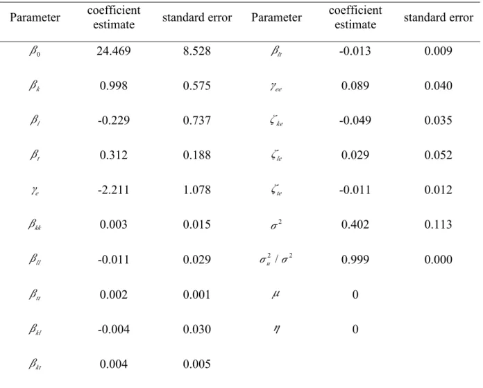
All estimated parameters are summarized in Table 2, which are used in the following to generate theTE and non-adjusted EE scores.

(16)

Table 1: Tests of hypothesis for parameters Specification Null hypothesis Tested against Log likelihood Likelihood ratio 2 Prob> χ Decision 1. Truncated-normal stochastic 313.671 2. Absence of Uit 0 γ= 1 _-2.215 _631.771 _0.000 _rejected 3. Half-normal μ =0 1 323.305 0.732 0.694 accepted 4. Time-invariant 0, 0 μ= η= 3 _312.035 _2.540 _0.111 _accepted

Table 2: Parameter estimates

Parameter coefficient

estimate standard error Parameter

coefficient

estimate standard error

0 β 24.469 8.528 βlt -0.013 0.009 k β 0.998 0.575 γee 0.089 0.040 l β -0.229 0.737 ζke -0.049 0.035 t β _0.312 _0.188 ζ_le _0.029 _0.052 e γ _-2.211 _1.078 ζ_te _-0.011 _0.012 kk β _0.003 _0.015 2 σ 0.402 0.113 ll β _-0.011 _0.029 2 _/ 2 u σ σ 0.999 0.000 tt β 0.002 0.001 μ 0 kl β -0.004 0.030 η 0 kt β 0.004 0.005

Note: The subscripts k, l, t and e refer to capital, labor, time trend, and energy consumption, respectively.

(17)

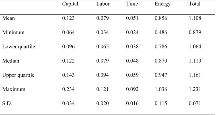
Table 3 reports elasticities of output with respect to each input. The sum of the mean output elasticities of four inputs indicates the presence of increasing returns to scale. The monotonicity assumption is violated for none of the inputs.

Table 3: Output elasticities

Capital Labor Time Energy Total

Mean 0.123 0.079 0.051 0.856 1.108 Minimum 0.064 0.034 0.024 0.486 0.879 Lower quartile 0.096 0.065 0.038 0.786 1.064 Median 0.122 0.079 0.048 0.870 1.119 Upper quartile 0.143 0.094 0.059 0.947 1.161 Maximum 0.234 0.121 0.092 1.036 1.231 S.D. 0.034 0.020 0.016 0.115 0.071

Estimated TE and EE are summarized in Tables 4 and 5. TE scores vary from 27.4% to 98.8%, with a mean of 63.4%, in line with the findings of Zhang (2009). Ningxia (27.4%), Guizhou (31.8%) and Qinghai (31.8%) have the lowest TE scores, all in west China. Meanwhile, Guangdong (98.8%), Beijing (98.1%) and Shanghai (97.6%), the most economically developed regions in China, have the highest TE scores. EE scores vary from 3.6% to 98.8%, with an overall mean of 57.3%. Over the period 2005-2010, Ningxia (7.3%), Qinghai (7.4%) and Gansu (21.1%) have the lowest mean EE scores, while Guangdong (98.8%), Beijing (97.4%) and Shanghai (97.0%) have the highest mean EE scores. Nevertheless, theseEE scores will be further adjusted.

(18)

Table 4: Estimates ofTE and non-adjusted EE

Technical efficiency Environmental efficiency

Overall mean 63.4% 57.3%

Overall minimum 27.4% 3.6%

Overall lower quartile 45.1% 41.0%

Overall median 61.2% 56.3%

Overall upper quartile 81.2% 76.4%

Overall maximum 98.8% 98.8%

Overall Standard Deviation (S.D.). 0.213 0.254

Overall observation number 180 177

Note: ThreeEEs cannot be solved.

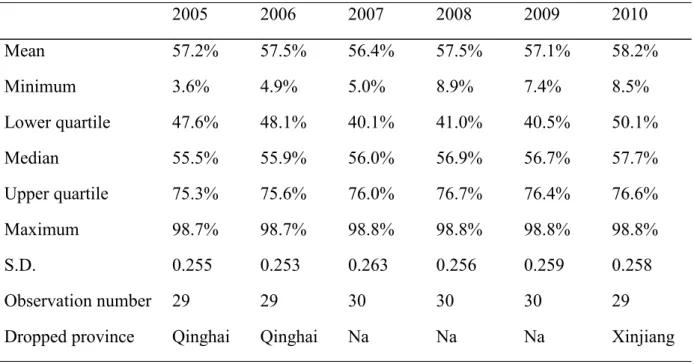
Table 5: Estimates of non-adjustedEE by year

2005 2006 2007 2008 2009 2010 Mean 57.2% 57.5% 56.4% 57.5% 57.1% 58.2% Minimum 3.6% 4.9% 5.0% 8.9% 7.4% 8.5% Lower quartile 47.6% 48.1% 40.1% 41.0% 40.5% 50.1% Median 55.5% 55.9% 56.0% 56.9% 56.7% 57.7% Upper quartile 75.3% 75.6% 76.0% 76.7% 76.4% 76.6% Maximum 98.7% 98.7% 98.8% 98.8% 98.8% 98.8% S.D. 0.255 0.253 0.263 0.256 0.259 0.258 Observation number 29 29 30 30 30 29

Dropped province Qinghai Qinghai Na Na Na Xinjiang

4.3. Effects of fiscal imbalance

Based on the second-stageEE model, EE scores are regressed against TR and FG. Among the set of control variables, income per capita (Dev) and population density (Density) are put in logarithm. In order to be in line with EKC studies, cubed and squared income per capita (Dev3 andDev2_{) are included.}

(19)

4.3.1. Linear effects ofTR and FG

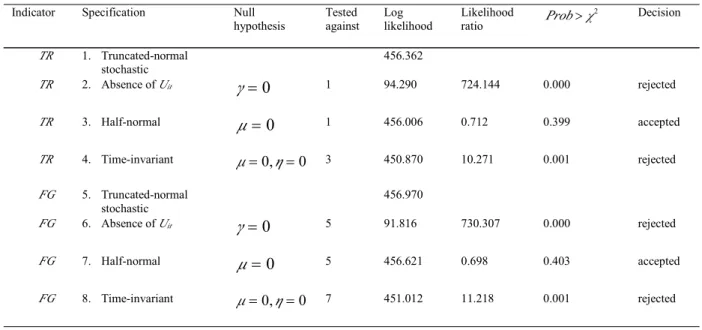
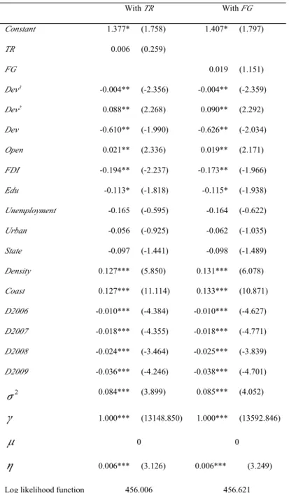
First, linear effects of TR and FG are tested for. I start with a time-variant model where the distribution of the one-sided error is normal-truncated. Specification tests statistics are summarized in Table 6. According to the LR tests, for both TR and FG, the null hypothesis of

0

γ= is strongly rejected, indicating the presence of stochastic errors and the necessary of the SFA model. The null hypothesis μ =0 can’t be rejected at 5% level of significance. The null hypothesis of η=0 is strongly rejected. As a result, the time-variant model with half-normal distribution is adopted for the second-stage SFA.

Table 6: Specification tests for the 2nd_{-stage linear effect model}

Indicator Specification Null hypothesis Tested against Log likelihood Likelihood ratio 2 Prob>χ Decision TR 1. Truncated-normal stochastic 456.362 TR 2. Absence ofUit γ₌₀ 1 94.290 724.144 0.000 rejected TR 3. Half-normal _μ ₌₀ 1 456.006 0.712 0.399 accepted TR 4. Time-invariant _μ₌_0,_η₌₀ 3 450.870 10.271 0.001 rejected FG 5. Truncated-normal stochastic 456.970 FG 6. Absence ofUit γ=0 5 91.816 730.307 0.000 rejected FG 7. Half-normal _μ ₌₀ 5 456.621 0.698 0.403 accepted FG 8. Time-invariant _μ₌_0,_η₌₀ 7 451.012 11.218 0.001 rejected

Estimation results are presented in Tables 7. Both TR and FG have positive and non-significant coefficients. These results suggest that fiscal imbalance don’t have any non-significant effects on EE, which seems to go against the prediction. However, insignificant linear effects of TR and FG are not surprising because it is reasonable to think that fiscal imbalance may have different effects on EE under different circumstances. For example, poor localities may be more vulnerable facing fiscal pressures and sacrifice more easily environment. As a result, in the following, nonlinear effects of TR and FG on EE will be considered. Concerning control variables, most of they have expected signs, among which squared income per capita, trade openness, population density and Coast dummy have positive and significant coefficients, while income per capita, cubed income per capita, FDI, illiterate rate and year dummies have negative and significant coefficients.

(20)

Table 7: Estimation with linearTR and FG effects WithTR WithFG Constant 1.377* (1.758) 1.407* (1.797) TR 0.006 (0.259) FG 0.019 (1.151) Dev3 _-0.004** _(-2.356) _-0.004** _(-2.359) Dev2 _0.088** _(2.268) _0.090** _(2.292) Dev -0.610** (-1.990) -0.626** (-2.034) Open 0.021** (2.336) 0.019** (2.171) FDI -0.194** (-2.237) -0.173** (-1.966) Edu -0.113* (-1.818) -0.115* (-1.938) Unemployment -0.165 (-0.595) -0.164 (-0.622) Urban -0.056 (-0.925) -0.062 (-1.035) State -0.097 (-1.441) -0.098 (-1.489) Density 0.127*** (5.850) 0.131*** (6.078) Coast 0.127*** (11.114) 0.133*** (10.871) D2006 -0.010*** (-4.384) -0.010*** (-4.627) D2007 -0.018*** (-4.355) -0.018*** (-4.771) D2008 -0.024*** (-3.464) -0.025*** (-3.839) D2009 -0.036*** (-4.246) -0.038*** (-4.701) 2 σ 0.084*** (3.899) 0.085*** (4.052) γ 1.000*** (13148.850) 1.000*** (13592.846) μ 0 0 η 0.006*** (3.126) 0.006*** (3.249) Log likelihood function 456.006 456.621

Note:t-student statistics between parentheses, *** significance at 1% level, ** significance at 5% level, * significance at 10% level.

4.3.2. Nonlinear effects ofTR and FG

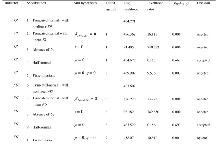
In order to examine potential nonlinear effects of TR and FG, interactions between fiscal imbalances and income per capita are created, namely TR∗Dev and FG∗Dev . These interactions allow testing whether effects of fiscal imbalances onEE in a province depend on

(21)

its economic development level.17_{The LR test statistics strongly reject the null hypothesizes} that the coefficients β_{TR DEV}_∗ and β_{FG DEV}_∗ (associated respectively to

TR∗DEV and FG∗DEV ) are equal to zero. This means that the specifications with interactions are more fit than those without interactions. Once again, the time-variant model with half-normal distribution is adopted. Specification tests statistics are summarized in Table 8. Regression results are presented in Table 9.

Table 8: Specification tests for the 2nd_{-stage nonlinear effect model}

Indicator Specification Null hypothesis Tested against Log likelihood Likelihood ratio 2 Prob>χ Decision TR 1. Truncated-normal with nonlinearTR 464.771 TR 2. Truncated-normal with linearTR 0 T R D EV β _∗ = 1 456.362 16.818 0.000 rejected TR 3. Absence ofUit γ =0 1 94.405 740.732 0.000 rejected TR 4. Half-normal μ =0 1 464.675 0.193 0.661 accepted TR 5. Time-invariant μ=0,η=0 3 459.907 9.536 0.002 rejected FG 6. Truncated-normal with nonlinearFG 463.607 FG 7. Truncated-normal with linearFG 0 F G D E V β _∗ = 6 456.970 13.274 0.000 rejected FG 8. Absence ofUit γ =0 6 92.182 742.850 0.000 rejected FG 9. Half-normal μ =0 6 463.529 0.156 0.693 accepted FG 10. Time-invariant μ=0,η=0 9 458.074 10.910 0.001 rejected

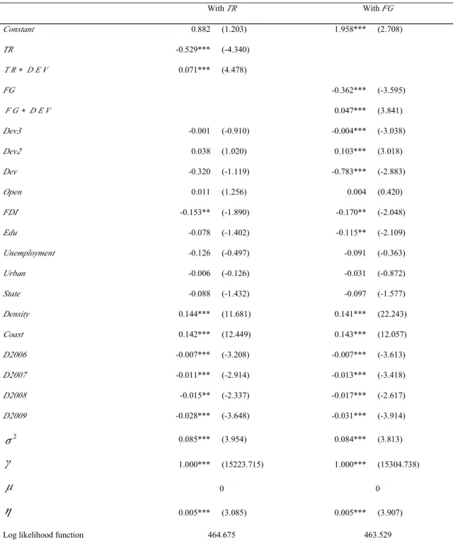
It is notable that when interactions are included, both TR and FG as well as their interactions with income per capita have significant coefficients, suggesting the significant nonlinear effects of fiscal imbalances onEE. Precisely, the marginal effects of TR and FG are conditional on income per capita. Their marginal effects are offset by economic development level, i.e., the more a province is affluent, the less fiscal imbalances are detrimental to EE,

17_{An important issue worth considering is the potential endogeneity of income per capita in the 2nd-stage model}

(Stern, 2004). Several alternative models i.e., IV estimator, lagged endogenous variables and control function method have been estimated in order to control the potential bias. All of these models give consistent results with

(22)

vice versa. These results seem to confirm the hypothesis that fiscal imbalances have more serious environmental consequences in poorer localities than in richer ones. In these two nonlinear-effect models, control variables have the same signs as in previous linear effect models, although different orders of income per capita become non-significant in TR regression.

Table 9: Estimates with nonlinearTR and FG effects

WithTR WithFG Constant 0.882 (1.203) 1.958*** (2.708) TR -0.529*** (-4.340) T R∗D E V 0.071*** (4.478) FG -0.362*** (-3.595) F G ∗D E V 0.047*** (3.841) Dev3 -0.001 (-0.910) -0.004*** (-3.038) Dev2 0.038 (1.020) 0.103*** (3.018) Dev -0.320 (-1.119) -0.783*** (-2.883) Open 0.011 (1.256) 0.004 (0.420) FDI -0.153** (-1.890) -0.170** (-2.048) Edu -0.078 (-1.402) -0.115** (-2.109) Unemployment -0.126 (-0.497) -0.091 (-0.363) Urban -0.006 (-0.126) -0.031 (-0.872) State -0.088 (-1.432) -0.097 (-1.577) Density 0.144*** (11.681) 0.141*** (22.243) Coast 0.142*** (12.449) 0.143*** (12.057) D2006 -0.007*** (-3.208) -0.007*** (-3.613) D2007 -0.011*** (-2.914) -0.013*** (-3.418) D2008 -0.015** (-2.337) -0.017*** (-2.617) D2009 -0.028*** (-3.648) -0.031*** (-3.914) 2 σ 0.085*** (3.954) 0.084*** (3.813) γ 1.000*** (15223.715) 1.000*** (15304.738) μ 0 0 η 0.005*** (3.085) 0.005*** (3.907) Log likelihood function 464.675 463.529

Note:t-student statistics between parentheses, *** significance at 1% level, ** significance at 5% level, * significance at 10% level.

(23)

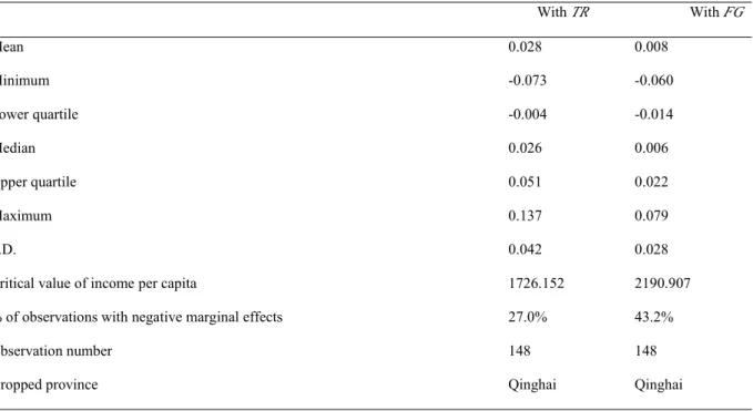
4.3.3. Marginal effects ofTR and FG

Overall marginal effects ofTR and FG are reported in Table 10. Critical values of income per capita below which the marginal effects are negative are also reported. It is notable that while both indictors have positive mean marginal effect on EE, an increase in fiscal imbalance is still detrimental to environment in a considerable number of the least affluent provinces (27% forTR and 43% for FG).

Table 10: Overall marginal effects of fiscal imbalances

WithTR WithFG Mean 0.028 0.008 Minimum -0.073 -0.060 Lower quartile -0.004 -0.014 Median 0.026 0.006 Upper quartile 0.051 0.022 Maximum 0.137 0.079 S.D. 0.042 0.028

Critical value of income per capita 1726.152 2190.907 % of observations with negative marginal effects 27.0% 43.2%

Observation number 148 148

Dropped province Qinghai Qinghai

Note: Critical value of income per capita is in 2005 USD.

5.

5.5.5. ConditionalConditionalConditionalConditional environmentalenvironmentalenvironmentalenvironmental efficiencyefficiencyefficiencyefficiency

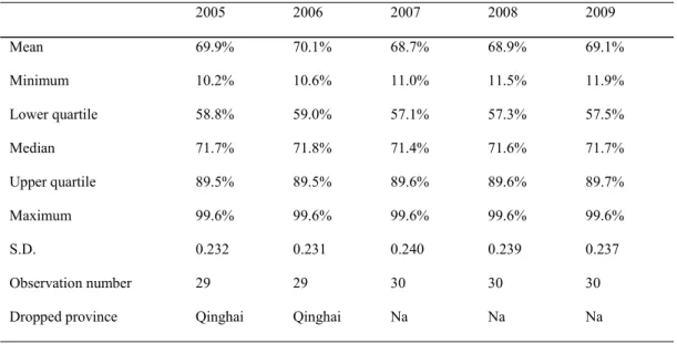
In this subsection,CEE scores are calculated using results of the second-stage SFA. Although consistent results have been found regarding nonlinear effects of TR and FG, the model with TR has higher log likelihood value. According to the Akaike information criterion (AIC), this model is preferred because it has a smaller AIC value. Thus, the adjusted environmental efficiency scores are calculated based on the two-stage SFA with TR. Summary of overall provincial CEE scores by region is presented in Table 11. It is remarkable that Chinese provinces have on average relatively higher EE scores once external variables are controlled. CEE scores vary from 10.2% to 99.6% with an overall mean of 69.3%. Among the seven regions, East China has the highest mean scores (84.2%), followed by South China (75.0%)

(24)

behind the others. Summary of CEE by year is presented in Table 12. It seems that CEE scores are relatively stable over this period. The three provinces with the highest mean CEE scores are Beijing (99.6%), Fujian (99.5%) and Jiangxi (99.5%). The three provinces with the lowest mean CEE scores are Ningxia (11.0%), Qinghai (27.0%) and Guizhou (30.6%). The concordance between EE ranking and CEE ranking is positive and significant. The Spearman rank correlation coefficient between the two measures is 0.715. The null hypothesis that the two rankings are independent can be strongly rejected. The entire rankings list of EE and CEE scores can be found in Appendix III.

Table 11: Summary of overall and regionalCEE scores

Overall North Northeast East Center South Southwest Northwest Mean 69.3% 63.2% 74.9% 84.2% 69.4% 75.0% 63.3% 51.2% Minimum 10.2% 32.0% 53.6% 56.7% 62.3% 58.8% 29.9% 10.2% Lower quartile 57.4% 40.8% 54.2% 75.4% 62.9% 59.4% 47.2% 26.7% Median 71.8% 68.2% 72.0% 88.9% 70.9% 70.9% 66.6% 40.0% Upper quartile 89.6% 74.5% 98.8% 99.5% 74.6% 94.8% 79.7% 73.4% Maximum 99.6% 99.6% 98.8% 99.5% 75.0% 94.9% 89.7% 95.5% S.D. 0.233 0.246 0.191 0.141 0.052 0.154 0.218 0.321 Nb. of ob. 148 25 15 35 15 15 20 23 Dropped province Na Na Na Na Na Na Na Qinghai

Table 12: Summary ofCEE by year

2005 2006 2007 2008 2009 Mean 69.9% 70.1% 68.7% 68.9% 69.1% Minimum 10.2% 10.6% 11.0% 11.5% 11.9% Lower quartile 58.8% 59.0% 57.1% 57.3% 57.5% Median 71.7% 71.8% 71.4% 71.6% 71.7% Upper quartile 89.5% 89.5% 89.6% 89.6% 89.7% Maximum 99.6% 99.6% 99.6% 99.6% 99.6% S.D. 0.232 0.231 0.240 0.239 0.237 Observation number 29 29 30 30 30 Dropped province Qinghai Qinghai Na Na Na

(25)

6.

6.6.6. ConcluConcluConcluConclusionsionsionsion

Decentralization has been promoted by major international institutions. Proponent arguments defending the merits of decentralization are abundant. However, many studies show that decentralization may be inefficient for environmental protection. China’s one-sided fiscal decentralization has shown an example. After 1994, public expenditures are largely decentralized while fiscal revenues are recentralized. Sub-national, in particular sub-provincial governments have excessively heavy expenditure responsibilities which are mismatched with their revenue assignments. Sub-national governments have huge fiscal imbalances and depend basically on transfers to fulfill their expenditure responsibilities. It seems that this critical situation may have negative effects on environmental protection. Localities, especially poor ones, are likely to under-provide environmental protection service either due to incapacity or incentive to develop economy at the cost of environment.

In this paper, I study empirically the environmental effect of this one-sided fiscal decentralization. Precisely, I examine whether fiscal imbalances caused by this decentralization improve or reduce environmental efficiency of Chinese provinces. Following the two-stage EE model of Reinhard et al. (2000), I first calculate with EE scores of Chinese provinces’ gross regional product over the period 2005-2010. After that, EE scores are regressed against two fiscal imbalance indicators, TR and FG, in order to test the linear and nonlinear effects of the latter. Finally, adjusted EE scores are calculated conditional on fiscal imbalances and other underground variables.

The empirical results are interesting to interpret. During the period of study, fiscal imbalances have nonlinear effects on EE of Chinese provinces. Moreover, these effects seem to be conditional on economic development level, i.e., fiscal imbalances seem to be more detrimental in less affluent provinces, which confirm the vulnerability of poor localities in face of severe fiscal pressures. In at least 27% of the cases, larger fiscal imbalances reduceEE. Once external factors are controlled, Chinese provinces have on average an adjustedEE score of 69.3%, considerably higher than 57.3% before the adjustment. This increase suggests that the overall external context in China contributes to environmental inefficiency. If all provinces had the same external context as the most advantageous one, mean EE would increase from 57.3% to 69.3%.

(26)

Results obtained in this paper call for attention to the potential negative environmental effects of the one-sided fiscal decentralization in poor provinces. Too many responsibilities without adequate revenues can lead to inefficient resource allocation; severe fiscal pressures may encourage poor localities to engage in short-term behaviors, e.g. developing economy at the cost of environment. Moreover, since the effects are nonlinear, it seems that this fiscal decentralization has regressive environmental effects in contributing to disparity across regions in terms of sustainable development. Although the choice between more revenue autonomy and less expenditure responsibilities is still a political debate in China, it is certain that the balance between expenditure responsibilities and revenue assignments need to be redressed for a more sustainable regional development in this country.

References: References:References:References:

Aigner, D., Knox Lovell, C.A., Schmidt, P., 1977. Formulation and estimation of stochastic frontier production function models. Journal of Econometrics 6(1), 21-37.

Battese, G.E, Coelli, T.J., 1995. A model for technical inefficiency effects in a stochastic frontier production function for panel data. Empirical Economics 20(2), 325-32.

Battese, G.E, Coelli, T.J., 1988. Prediction of firm-level technical efficiencies with a generalized frontier production function and panel data. Journal of Econometrics 38(3), 387-399.

Beeson, P.E., Husted, S., 1989. Patterns and determinants of productive efficiency in state manufacturing. Journal of Regional Science 29(1), 15-28.

Cai, Y., Liu, X, 2010. Provincial tax competition and environmental pollution: based on panel data from 1998 to 2006 in China. Journal of Finance and Economics 36(4).

Charnes, A., Cooper, W.W., Rhodes, E., 1978. Measuring the efficiency of decision making units. European Journal of Operational Research 2(6), 429-444.

Christensen, L.R., Jorgenson, D.W., Lau, L.J., 1971. Conjugate duality and the transcendental logarithmic production function. Econometrica 39, 28-45.

Coelli, T.J., 1996. A Guide to FRONTIER Version 4.1: A computer program for stochastic frontier production and cost function estimation, Department of Econometrics, University of New England.

(27)

Cooper, W.W., Seiford, L.M., Tone, K., 2006. Data envelopment analysis: A Comprehensive Text with Models, Applications, References and DEA-Solver Software 2nd ed., Springer.

Cuesta, R.A., Knox Lovell, C.A., Zofío, J.L., 2009. Environmental efficiency measurement with translog distance functions: A parametric approach. Ecological Economics 68(8/9), 2232-2242.

Dasgupta, S., Laplante, B., Mamingi, N., Wang, H., 2001. Inspections, pollution prices, and environmental performance: evidence from China. Ecological Economics 36(3), 487-498.

Fried, H.O., Lovell, C.A.K., Schmidt, S.S., Yaisawarng, S., 2002. Accounting for environmental effects and statistical noise in data envelopment analysis. Journal of Productivity Analysis (17), 157–174.

Gangadharan, L., Valenzuela, M.R., 2001. Interrelationships between income, health and the environment: extending the Environmental Kuznets Curve hypothesis. Ecological Economics36(3), 513-531.

Greene, W.H., 1999. Frontier Production Functions. In: M. Hashem Pesaran and P. Schmidt (eds) Handbook of Applied Econometrics Volume II: Microeconomics, Balckwell Publishers, Massachusetts.

Hailu, A., Veeman, T.S., 2001. Non-parametric productivity analysis with undesirable outputs: an application to the Canadian pulp and paper industry. American Journal of Agricultural Economics 83(3), 605-616.

Hjalmarsson, L., Kumbhakar, S.C., Heshmati, A., 1996. DEA, DFA and SFA: A comparison. Journal of Productivity Analysis 7, 303-327.

Isaksson, A., 2007. Determinants of total factor productivity: a literature review, United Nations Industrial Development Organization (UNIDO).

Jiang, H., 2006. Decentralization, ecological construction, and the environment in post-reform China: Case study from Uxin Banner, Inner Mongolia. World Development 34(11), 1907-1921.

Jing, Y., Liu, X., 2009. Intergovernmental fiscal relations in China: An assessment. In Local Governance under Stress: Fiscal Retrenchment and Expanding Public Demands on

(28)

Li, Y., Hu, J.L., 2002. Technical efficiency and location choice of small and medium-sized enterprises. Small Business Economics 19(1), 1-12.

Meeusen, W., van den Broeck, J., 1977. Efficiency estimation from Cobb-Douglas production functions with composed error. International Economic Review 18(2), 435-444.

Mkhabela, T., 2011. An econometric analysis of the economic and environmental efficiency of dairy farms in the KwaZulu-Natal Midlands. PH.D. thesis, Stellenbosch University.

Qian, Y., Roland, G., 1998. Federalism and the Soft Budget Constraint. The American Economic Review 88(5), 1143-1162.

Reinhard, S., Knox Lovell, C.A., Thijssen, G.J., 2000. Environmental efficiency with multiple environmentally detrimental variables; estimated with SFA and DEA. European Journal of Operational Research 121(2), 287-303.

Reinhard, S., Knox Lovell, C.A., Thijssen, G.J., 2002. Analysis of environmental efficiency variation. American Journal of Agricultural Economics 84(4), 1054-65.

Reinhard, S., Knox Lovell, C.A., Thijssen, G.J., 1999. Econometric estimation of technical and environmental efficiency: An application to dutch dairy farms. American Journal of Agricultural Economics 81(1), 44-60.

Söderbom, M., Teal, F., 2004. Size and efficiency in African manufacturing firms: evidence from firm-level panel data. Journal of Development Economics 73(1), 369-394.

Stern, D.I., 2004. The rise and fall of the Environmental Kuznets Curve. World Development 32(8), 1419-1439.

Wang, H., Wheeler, D., 2003. Equilibrium pollution and economic development in China. Environment and Development Economics 8(03), 451-466.

Wang, H., Wheeler, D., 2005. Financial incentives and endogenous enforcement in China’s pollution levy system. Journal of Environmental Economics and Management 49(1), 174-196.

World Bank, 2002. China: National development and sub-national finance: a review of provincial expenditures, Poverty Reduction and Economic Management Unit, East Asia and Pacific Region. The World Bank.

(29)

Wu, Y., 2010. Regional environmental performance and its determinants in China. China & World Economy 18, 73-89.

Yang, H., Pollitt, M., 2009. Incorporating both undesirable outputs and uncontrollable variables into DEA: The performance of Chinese coal-fired power plants. European Journal of Operational Research 197(3), 1095-1105.

Yuan, P., Cheng, S., 2011. Examining Kuznets Curve in environmental efficiency of China’s industrial sector. China Industrial Economics 2011(02).

Zhang, B., Bi, J., Fan, Z., Yuan, Z., Ge, J., 2008. Eco-efficiency analysis of industrial system in China: A data envelopment analysis approach. Ecological Economics 68(1-2), 306-316.

Zhang, J., Wu, G.Y., Zhang, J.P., 2004. The Estimation of China’s provincial capital stock: 1952—2000. Economic Research Journal 2004(10).

Zhang, T., 2009. Frame work of data envelopment analysis—A model to evaluate the environmental efficiency of China’s industrial sectors. Biomedical and Environmental Sciences 22(1), 8-13.

Zhang, T., Xue, B.D., 2005. Environmental efficiency analysis of China’s vegetable production. Biomedical and Environmental Sciences 18(1), 21-30.

Zhou, P., Ang, B.W., Poh, K.L., 2008. A survey of data envelopment analysis in energy and environmental studies. European Journal of Operational Research 189(1), 1-18.

(30)

Appendices:

Appendix I: Name and description of variables

Variable Description

Y

Gross regional product (10000 USD at 2005 price)

K Provincial capital stock (10000 RMB at 1952 price)

L Total provincial employment at the end of year (10000 persons)

T Time trend

E

Total energy consumption ( ton of Standard Coal Equivalent)

TR

Share of central transfers in provincial expenditures

FG Fiscal gap

Dev Income per capita (2005 USD)

Open (Exportation + Importation)/ Gross regional product

FDI Foreign direct investments/ Gross regional product

Edu Illiterate rate

Unemployment Unemployment rate

Urban Non-agricultural population/total population

State Employment of state-owned sector/total employment

Density Population /km2

Coast 1 if coast province, 0 otherwise

D2006 1 if the year of 2006, 0 otherwise

(31)

Appendix II: Summary statistics of variables

Variable Obs. Mean S.D. Min Max

Y 180 14300000 12900000 663023 69500000 K 180 54300000 49100000 3714443 263000000 L 180 2423.416 1602.439 267.619 6041.557 T 180 3.500 1.713 1 6 E 179 138000000 94900000 8221845 497000000 TR 148 0.509 0.183 0.141 0.857 FG 148 0.478 0.182 0.078 0.818 Dev 148 3102.874 2125.191 616.500 11862.610 Open 148 0.359 0.410 0.045 1.668 FDI 148 0.026 0.020 0.001 0.082 Edu 148 0.088 0.046 0.028 0.223 Unemployment 148 0.038 0.006 0.014 0.056 Urban 148 0.367 0.164 0.158 0.880 State 148 0.111 0.048 0.053 0.245 Density 148 411.474 534.697 7.667 3029.969 Coast 148 0.372 0.485 0 1 D2006 148 0.196 0.398 0 1 D2007 148 0.203 0.403 0 1 D2008 148 0.203 0.403 0 1 D2009 148 0.203 0.403 0 1

(32)