Multivariate modeling of glacimarine lithostratigraphy combining scanning XRF, multisensory core properties, and CT imagery: IODP Site U1419

Research Paper

1

GEOSPHERE| Volume 14 | Number 4

Multivariate modeling of glacimarine lithostratigraphy combining

scanning XRF, multisensory core properties, and CT imagery:

IODP Site U1419

Michelle L. Penkrot

_{, John M. Jaeger}

_{, Ellen A. Cowan}

_{, Guillaume St-Onge}

_{, and Leah LeVay}

1_{Department of Geological Sciences, University of Florida, Gainesville Florida 32611-2120, USA}

2_{Department of Geological and Environmental Sciences, Appalachian State University, Boone, North Carolina 28608, USA}

3_{Institut des sciences de la mer de Rimouski (ISMER), Canada Research Chair in Marine Geology, Université du Québec à Rimouski and GEOTOP, Rimouski, QC G5L 3A1, Canada} 4_{International Ocean Discovery Program, Texas A&M University, College Station, Texas 77845, USA}

ABSTRACT

Marine sediments preserve archives of glacier behavior from many proxies, with lithofacies analysis providing direct evidence of glacial extent and dynamics. Many of these lithofacies have corresponding physical and geochem-ical properties that may be identified through quantitative, nondestructive log-ging properties. This study applies supervised and unsupervised classification to downcore logging data to attempt to model temperate glacimarine facies, which are independently identified via visual lithofacies analysis based on core photographs, digital X-radiography, and computed tomography scans. We test the limits of these methods by modeling both broad glacial and interglacial and small-scale variations in Late Pleistocene (<60,000 yr) glacier extent leading into the Holocene deglaciation for a temperate ice stream at Integrated Ocean Drilling Program Site U1419 in the Gulf of Alaska. Multi-meter–scale mud and diamict lithofacies interpreted as non-glacial versus glacial conditions can be modeled with both methods using downcore physical property logging data (b* color reflectance, magnetic susceptibility, and natural gamma- ray activ-ity) augmented with scanning X-ray fluorescence (XRF) elemental abundance (Ca, Zr, Si, K, Rb, and Al). Physical properties are most useful for delineating decimeter-meter–scale variations in composition and clay content, whereas scanning XRF elements best capture differences in sand versus clay content and composition at decimeter-centimeter scales. Neither classification tech-nique can model the observed small-scale variations in diamict facies using elemental abundance from higher-resolution scanning XRF or from physical properties. Comparison of unsupervised cluster model results with observed lithofacies allows for identification of three different glacial conditions at Site U1419—ice-proximal, fluctuating, and retreating. For small-scale variations in glacial extent, cluster model results are best used as complementary data to image-based lithofacies identification rather than as a replacement.

INTRODUCTION

Variations in ice sheet and glacier extent are a dynamic component of Earth’s climate system. Study of glacial dynamics during major climate tran-sitions helps establish ice sheet “tipping points” (Lenton et al., 2008; Kriegler

et al., 2009) and for predicting how modern ice sheets and glaciers may re-spond to our warming climate. The marine sediment record provides a highly detailed archive of glacial dynamics through a combination of glacial extent proxies, such as lithofacies, biogenic carbonate chemistry, productivity, and mass accumulation rates (Andersen et al., 1996; Andrews and Principato, 2002; Naish et al., 2009; Ó Cofaigh et al., 2013). Of these proxies, lithofacies analysis provides one of the most direct records of glacial extent because spatial and temporal variations are recorded as spatial transitions in facies. The transition between glacial and interglacial states is interpreted from lithofacies across the globe (e.g., Henrich et al., 1989; Peterson et al., 2000), with the most obvi-ous examples from glaciated continental margins (Ó Cofaigh and Dowdeswell, 2001). Open-water, nonglacial conditions most often result in accumulation of homogeneous, bioturbated mud with a varying biogenic component, whereas glacial conditions are recognized by heterolithic facies with abundant lone-stones. In particular, temperate glacimarine strata contain evidence of abun-dant ice rafting, gravity flows, and meltwater-derived sediment that provide a wide potential range of distinctive lithofacies throughout a glacial-interglacial cycle (Powell and Cooper, 2002) (Fig. 1).

Glacimarine lithofacies are typically recognized in outcrop and core through visual lithostratigraphic logging, which can be augmented using more quantitative methods. Visual core descriptions (VCDs) are based on sediment texture, composition, color, and physical and biogenic sedimentary structures. Computed tomography (CT) scan images and X-radiographs contribute de-tails on subtle features within cores (Cnudde and Boone, 2013). Although CT imagery is ideal for identification and description of a myriad of glacimarine sedimentary features (Boespflug et al., 1995; Gagnoud et al., 2009; St-Onge and Long, 2009; Davies et al., 2011; Tarplee et al., 2011), this technology is ex-pensive and/or of restricted availability. Fortunately, many of the same visual features also have corresponding physical and geochemical properties that may be identified through quantitative nondestructive logging properties such as natural gamma radiation, color reflectance, bulk density, magnetic susceptibility, elemental concentration, etc. Logging data have been used to identify major end-member lithologies through supervised (e.g., support vector machine [SVM]; Hall, 2016) and unsupervised classification techniques (e.g., cluster analysis) for continental shelf environments (Inwood et al., 2013),

GEOSPHERE

https://doi.org/10.1130/GES01635.1 13 figures; 7 tables; 1 set of supplemental files CORRESPONDENCE: mpenkrot@ ufl .edu CITATION: Penkrot, M.L., Jaeger, J.M., Cowan, E.A., St-Onge, G., and LeVay, L., 2018, Multivariate modeling of glacimarine lithostratigraphy combining scanning XRF, multisensory core properties, and CT imagery: IODP Site U1419: Geosphere, v. 14, no. 4, p. 1–26, https://doi.org/10.1130/GES01635.1. Science Editor: Shanaka de Silva Associate Editor: Anthony E. Rathburn Received 13 November 2017 Revision received 21 March 2018 Accepted 11 June 2018

OPEN ACCESS

GOLD

This paper is published under the terms of the CC-BY-NC license.

Research Paper

2

GEOSPHERE| Volume 14 | Number 4

trench sediments (Tudge et al., 2009), and glacial sediments (Williams et al., 2012; Hunze et al., 2013). Classification techniques using multivariate data are powerful analytical tools in the geosciences because they provide a quantita-tive, objecquantita-tive, and reproducible approach to lithofacies analysis (Davis, 2002; Dubois et al., 2007).

In this study, we attempt to model temperate glacimarine lithofacies using supervised and unsupervised classification techniques applied to downcore logging data. Model results are validated through comparison to  lithofacies identified from a visual facies analysis of core photographs, CT scans, and X-radiographs. The goal is to test the limits of these classifica-tion techniques in identifying lithofacies representing both glacial and inter-glacial, and small-scale variations in glacier extent within hetero geneous diamict for a temperate glacial setting in the Gulf of Alaska, Integrated Ocean Drilling Program (IODP) Site U1419 (Fig. 2). Based on the shipboard age model, IODP Site U1419 extends back to the Late Pleistocene (<60,000 yr; Jaeger et al., 2014) and contains a last glacial maximum (LGM) to Holocene deglaciation sequence based on comparison with a neighboring well-dated core (Davies et  al., 2011). These modeling techniques may identify subtle lithofacies variations and provide an alternative to using costly CT scans and/or X-radiographs to highlight features not otherwise observable from split core surfaces during VCD. Integration of scanning XRF data also informs on downcore compositional changes that are geochemical rather than visual and are typically observed in smear slides. Classification analyses also

pre-sent a reproducible approach to categorizing core properties. A secondary objective is to test how different types of core logging data (i.e., physical properties versus elemental composition) and classification routine (e.g., supervised discriminant and SVM; unsupervised hierarchical versus model clustering) affect the classification analysis results. Previous studies using cluster analysis to identify glacial lithofacies used wireline downhole logging data (Williams et al., 2012; Hunze et al., 2013), which are not always collected in association with coring. This study tests the ability of logging data that are commonly collected on sediment cores (i.e., magnetic susceptibility, natural gamma radiation, color, scanning X-ray fluorescence) to predict lithofacies. When applying classification techniques to geologic data, there is still ambi-guity over which method provides the most valid results (Templ et al., 2008); thus this study applies common classification techniques to evaluate their utility in glacimarine studies.

METHODS

CT Imagery and Digital X-Radiography

Computed tomography (CT) scan images and X-radiographs of sediment cores allow for a detailed, nondestructive view of the entire core (e.g., St-Onge et al., 2007); this view is useful for identifying textural features such as sedi-mentary structures (Van Daele et  al., 2014), bioturbation (Gagnoud et  al., 2009), variations in sediment density (Ashi, 1997), and ice-rafted debris (IRD; Andrews and Principato, 2002; Jennings et al., 2018). Computed tomography

Grounded ice-margin Turbid overflow plume

Tidal currents Mass-flow

Distal Proximal Marginal Ice-contact Undeformed substrate Glacitectonite Laminated deformation till Coarse-grained subaqueous outwash Interlaminated sand & mud/laminated mud Mass-flow deposits including laminated muddy turbidites

Bioturbated massive mud

B A

Figure 1. Schematic diagram of glacimarine sedimentation typically found at temperate glacier- ocean interfaces. Lithology can be used as a proxy for the relative proximity of glacier terminus to core site. Stratified diamicts (A) are deposited proximally from increased sedimentation from meltwater discharge. Massive bioturbated muds (B) are created when the terminus is distal and sedimentation rates are low. Modified from Ó Cofaigh and Dowdeswell (2001). X-radiographs from Cowan et al. (1997) and Jaeger and Nittrouer (2006).

50 25 0 100 Km U1420 U1421

U1419

Bering

Gl.

Bagley Icefield

Figure 2. Regional bathymetric map of the Gulf of Alaska offshore of the Bering Glacier showing the location of Sites U1419, U1420, and U1421 drilled by Integrated Ocean Drilling Program (IODP) Expedition 341. Dashed line represents the estimated maximum ice extent during the last glacial maximum (LGM) from Kaufman and Manley (2004).

Research Paper

3

GEOSPHERE| Volume 14 | Number 4

scan images are cross-sectional slices of the core volume (Ketcham, 2005); while X-radiographs present an integrated view of the whole volume imaged.

U-channels from Site U1419 composite splice sections (Jaeger et al., 2014) were scanned at the Institut National de Recherche Scientifique–Eau Terre Envi ronnement (INRS-ETE, Quebec City, Canada) using a Siemens SOMATOM Definition AS+ 128 CAT-scanner with a current range of 300 mA and a voltage of 140 kV. X-radiograph images were collected on the archive halves of Site U1419 at the IODP Gulf Coast Repository at Texas A&M University using a digi-tal X-ray panel and veterinary X-ray unit (Walsh et al., 2014) on core sections that required additional imaging of a wider field of view to better discriminate features.

Downcore Logging

Downcore logging data are collected directly on whole and half-round core sections. This study uses downcore logging data commonly collected during and after IODP expeditions: physical properties and scanning X-ray fluores-cence (XRF) elemental data.

Physical Properties

Physical properties were rapidly measured shipboard to relate with core lith ology (Jaeger et al., 2014). Three of these properties—b* color reflectance, volume-normalized magnetic susceptibility (MS), and volume-normalized natural gamma radiation (NGR)—are used in this study as cluster model inputs. Magnetic susceptibility in a sediment core is a measure of how magnetized the sediment becomes when exposed to an external magnetic field (Hatfield et al., 2013). It is often used as a proxy for changes in sediment composition and lithology (Blum, 1997; Jessen et al., 2010). Regionally in the Gulf of Alaska, MS has been shown to covary with grain size; low MS values are found in clay-rich sediment and high MS values with sandy and silty sediments (Fig. 3; Cowan et al., 2006; Jaeger and Kramer, 2014; Walczak et al., 2017). NGR is naturally occurring gamma- ray radiation derived from K, U, and Th (Blum, 1997). It is a common tool used for interpreting lithology because K and Th are gener-ally concentrated in clay minerals; thus, high NGR values indicate a more clay-rich lithology (Blum, 1997). Both MS and NGR data sets used in this study are volume normalized to account for variable filling of core liners (Walczak et al.,

50 450 65 0 250 550 75 09 50 85 01 05 0 350 150 1.15 1.25 1.35 Green/Blue (RGB value) 2Biogenic silica (wt%)4 6 8 10 200 600 1000

Mag Sus (SI Units) 100000 250000Zr/K 0.00060 0.00075

Rb/Al

Depth (cm)

85JC

A B C D E F

Figure 3. Downcore properties from core EW0408-85JC co-located with Site U1419. (A) Computerized tomographic (CT) scans where warm colors (yellow and red) indi-cate higher densities, and cooler colors (blue and purple) indicate lower densi-ties. (B) Green-blue pixel intensity values from line-scan red-green-blue (RGB) color imagery; (C) biogenic silica concentra-tion; (D)  volume magnetic susceptibility; (E–F) elemental ratios from inductively coupled plasma–mass spectrometry data. Modified from Barron et al. (2009), Davies et al. (2011), and Addison et al. (2012).

Research Paper

4

GEOSPHERE| Volume 14 | Number 4

2015). The b* color reflectance represents sediment color on the Inter national Commission on Illumi nation (CIE) color space; blue (negative) to yellow (posi-tive) scale (Blum, 1997). Within Site U1419, sediment with higher b* values ap-pears greener in core photographs. Variations in color reflectance have been correlated with lithologic changes primarily due to changes in productivity (Vidal et al., 1998; Peterson et al., 2000; Nederbragt et al., 2006; Pan and Chen, 2013), with higher b* values (greener) associated with periods of increased diatom pro-ductivity (Nederbragt and Thurow, 2001; Debret et al., 2006; Debret et al., 2011). At Site U1419, quantitative color from RGB values of digital line scan images of core EW0408 85JC shows this relationship of greener sediments with higher biogenic silica concentrations (Fig. 3; Addison et al., 2012). Magnetic susceptibil-ity and NGR are measured on an 8-cm- and 10-cm-long whole-core volume and b* every 2 cm on the split core surface (Jaeger et al., 2014).

Scanning X-Ray Fluorescence

Scanning XRF elemental data were collected approximately every 2  cm, post-cruise on the Site U1419 composite spliced core (Penkrot et al., 2017a). To account for core surface inhomogeneity in grain size and porosity, which affects X-ray attenuation (Tjallingii et al., 2007), the scanning XRF data were calibrated with the normalized median-scaled method (NMS; Lyle et al., 2012). Ninety-five discrete bulk samples representing the full range of lithologies within Site U1419 were analyzed for major, minor, and trace elements via fused bead XRF analysis (Yamada, 2010; Watanabe, 2015) and an Element 2 inductively coupled plasma–mass spectrometer (ICP-MS) (Kamenov et al., 2009) at the University of Florida. Analytical uncertainty for all elements is better than ±5%. Normal-ized scanning XRF data for each element used are available in Supplemental File S11_{. Elements used for classification analysis are restricted to those most}

sensitive to grain-size variations (Al, Ca, K, Si, Rb, and Zr; Rothwell et al., 2006; Rothwell and Croudace, 2015). Elemental ratios of these elements successfully capture major lithologic changes in core EW0408 85JC (Fig. 3; Barron et al., 2009). Elements sensitive to changes in provenance (e.g., light rare-earth ele-ments [LREEs], Sc, Th, etc.; McLennan, 1989; Kaiser et al., 2007) and digenesis (e.g., Mo, V, Fe, etc.; Piper, 2001; Barron et al., 2009) are avoided.

Bulk Mineralogy

Bulk-sample X-ray diffraction patterns were collected shipboard for miner-alogy (Jaeger et al., 2014). Quantitative analyses of these scans were performed using the RockJock program in standardless analysis mode (Eberl, 2003).

Lithofacies Classification Analyses

Access to high-level computing and high-resolution sedimentary prop-erty data have driven many approaches that use machine learning to classify sedimentary facies from multivariate data sets. Most attempts have focused on classifying bulk sedimentary facies (e.g., mudstone, sandstone, marl, and

limestone) and have had varying success when models are validated against observed lithofacies (Dubois et  al., 2007; Hall, 2016; Sahoo and Jha, 2017). Successful attempts occur when there are numerous samples of classified data to use in training sets and lithofacies criteria are primarily compositional and/or mineralogical, which allows for effective classification by proxies such as natural gamma-ray logs (Benaouda et al., 1999; Dubois et al., 2007; Tang and White 2008).

The two modeling approaches used are supervised and unsupervised classi fication. In the former, algorithms are supplied with classified training data that let the model learn the relationships between the measurements and the classes (lithofacies), which are then assigned to unclassified mea-surements (Benaouda et al., 1999; Davis, 2002; Dubois et al., 2007; Tang and White, 2008). Unsupervised classification of lithofacies generally groups, or clusters, samples together based on common traits with a goal of maximiz-ing the difference between groups. A primary limitation of this approach is that the number of groups is not known in advance, and interpretation of the clusters in terms of controlling factors can be ambiguous (Templ et al., 2008; Ellefsen et al., 2014). A potential benefit of applying both approaches is that the supervised classification can objectively highlight the parameters or variables that best correlate with individual lithofacies, which can later help interpret the unsupervised clustering results.

Supervised Classification-Discriminant Analyses

Linear and quadratic discriminant analyses (LDA and QDA) result in classi-fication boundaries based on the calculation of discriminant scores that assign observations to a specific group (Davis, 2002). The LDA scores are calculated by finding linear combinations of the independent variables providing linear decision boundaries that assume equal covariance of variables in all groups. The QDA relaxes the requirement of equal covariance and is able to provide more accurate nonlinear, quadratic classification boundaries. Both techniques require Gaussian distributions of parameter values within groups; so outliers need to be eliminated and the distribution of each variable analyzed for each group (lithofacies) to test for normality. In general, QDA is less restrictive than LDA, but because it has a larger number of parameters to fit in its calculation, it requires larger data sets for the given number of groups and/or variables being analyzed. Both techniques use a Bayesian approach to provide a probability of group membership.

Supervised Classification-Support Vector Machines

Support vector machines (SVMs) have evolved to be the most flexible and used machine learning approach for supervised learning. This popularity arises because it requires fewer parameters to be fitted in the model and is less restrictive than LDA or QDA. Although as with all regression approaches, outliers in the data will reduce model accuracy. Within a SVM, data points are projected into higher-dimensional space using the kernel approach, where the 1_{Supplemental Materials. Figures S1–S5:}

Supple-mental figures present box-plots of logging data grouped by observed lithofacies, and mud-diamict and diamict- only clusters. In addition, they show Bayesian information criterion (BIC) plots for the most accurate unsupervised clustering results and crossplots of b* vs. MS. File S1: Supervised and un-supervised classification R code. File S2: Basic statis-tical parameters for the logging data. File S3: Ship-board collected mineralogy RockJock results. Please visit https:// doi .org /10 .1130 /GES01635 .S1 or access the full-text article on www .gsapubs .org to view the Supplemental Materials.

Research Paper

5

GEOSPHERE| Volume 14 | Number 4

points effectively become linearly separable into different classes. The optimal hyperplane between the groups (lithofacies) establishes the edges between the closest points of the classes, with points falling on the wrong side of the classification weighted down to minimize their importance of setting bound-aries. A subset of training points provides the probability of group member-ship through a computationally expensive cross-validation approach, which in the past has been a primary restriction on the use of SVMs.

Unsupervised Cluster Analysis

Clustering is a common multivariate statistical method that is useful for grouping observations into homogeneous clusters. Two different clustering routines are applied to the downcore logging data—hierarchical clustering and model clustering. Both routines have been applied to geochemical and logging data (Templ et al., 2008; Hunze et al., 2013; Ellefsen et al., 2014), with no con-sensus on the ideal clustering technique for these data types.

Hierarchical clustering is based on the multivariate distance between

ob-servations that can be either agglomerative or divisive. In this study, we apply an agglomerative approach using Euclidean distances and the Ward method (Ward, 1963) of clustering (Templ et al., 2008). This analysis was performed in the R programming language using the “hclust” function (R Core Team, 2017).

Model clustering is based on specific models that describe the multivariate

distribution of the data points forming clusters rather than on the distance between observations (Fraley and Raftery, 2002). In this study, we use a modi-fied mixture-model clustering method from Ellefsen et al. (2014) for geochem-ical data which is based on a finite mixture model that was first presented by Templ et  al. (2008). This analysis was performed in the R programming language using the “mclust” function (Fraley et al., 2012).

Supervised Classification Data Preparation

The accuracy of classification data analysis is highly dependent upon the inter group variance of the training data, which requires a robust evaluation of how the data fit the assumptions that are part of each analytical technique. Our data preparation procedures follow Gorman Sanisaca et  al. (2017), who use multi variate sediment data to assign membership to distinctive sources. All data preparation is performed using the statistical software R (R Core Team, 2017) and is presented in File S1 (footnote 1) for evaluation and implementation by others.

Data preparation involves screening data and then determining the opti-mal variables for use in classification algorithms. Because we use geochemical data in our model, we use preparation techniques appropriate for these closed data (i.e., expressed in units that sum to a constant; Davis, 2002; Templ et al., 2008). Data outliers are removed using the outCoDa function in the robCom-positions package in R, where outliers are detected based on (robust) Mahala-nobis distances after an isometric log-ratio transformation of the data (Filz-moser and Hron, 2008; Templ et al., 2011). This routine identified 28% of data as outliers (4661 used/6490 total). We test for any constant or almost constant

predictors across samples using the function nearZeroVar from the caret pack-age in R (Kuhn et al., 2017). Multivariate data sometimes contain predictors that take a unique value across samples (e.g., zero ppm concentrations), which add little discriminatory power to models and/or can complicate model result interpretations. A nonparametric Kruskal-Wallis test is used on each variable to see if the different lithofacies have unique values that allow for potential dis-crimination between lithofacies. Data are interrogated for collinearity (r >0.9) between variables, which can lead to serious stability problems in discrimi-nant function analyses (Davis, 2002). A Levene test is used to test for homo-geneity of variance (Gorman Sanisaca et al., 2017), which showed that several parameters (e.g., Ca and Zr) do not meet the LDA requirement of homogene-ity; therefore, only QDA techniques are used. Closed compositional data are opened for classified models using a center-log ratio transform (Templ et al., 2008). Physical property data were standardized (z-score) to account for differ-ences in measurement units when calculating distance coefficients (Milligan and Cooper, 1988; Kynčlová et al., 2016). Finally, for supervised classification models, we use a forward stepwise linear discriminant function approach to establish which parameters were most important in separating the lithofacies types using the function “greedy.wilks” in the R package klaR (Weihs et  al. 2005). These parameters are then grouped for analyses in QDA and SVM models. Supervised model accuracy is evaluated using a cross-validation ap-proach within the caret package in R (Kuhn et al., 2017). The number of training samples among the different lithofacies is balanced to prevent accuracy bias in the prediction model toward the most abundant lithofacies.

Unsupervised Clustering Procedure

Three physical properties (b*, MS, and NGR) and six elements (Al, Ca, Si, Rb, K, and Zr) were selected to be used as our multivariate cluster model in-puts. Both clustering routines were run with three different groups of input data: group 1 (G1)—physical properties and elemental data inputs (b*, MS, NGR, Al, Ca, Si, Rb, K, and Zr); group 2 (G2)—physical properties only (b*, MS, and NGR); group 3 (G3)—elemental data only (Al, Ca, Si, Rb, K, and Zr).

Prior to clustering, the input data were rescaled at a 2 cm resolution and treated to avoid artifacts. An isometric log-ratio (ilr) transformation was per-formed using the robCompositions R package (Templ et  al., 2011) on the NMS-normalized scanning XRF elements in order to open the data and remove the effects of a compositional closed data set (Templ et  al., 2008). Physical property data were normalized (z-score). Finally, the input data were trans-formed into robust (i.e., no outliers) principal components (Templ et al., 2011) before clustering to reduce dimensionality, which helps to reduce uncertainty encountered while clustering (Fraley and Raftery, 2002), remove correlation between input variables, and improve cluster stability (Ellefsen et al., 2014). These principal components were then used in hierarchical and modified mixture-model clustering routines written in R (File S1 [footnote 1]). For both clustering routines and each input variable group, the spatial relationship of the resultant clusters is plotted downcore, creating a cluster lithology column.

Research Paper

6

GEOSPHERE| Volume 14 | Number 4

RESULTS

Characterization of Observed Lithofacies

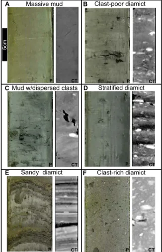
Twelve lithofacies are defined for Site U1419 based on shipboard visual core descriptions, smear slides, and core photographs supported by post-ex-pedition digital X-radiography and CT scans. Lithofacies are delineated based on sediment texture, color, degree of bioturbation, and sedimentary structures (Fig. 4 and Table 1). In general, these lithofacies match those identified ship-board (Jaeger et al., 2014). However, CT and X-radiograph imagery allows for better identification and subclassification of diamict lithofacies than visual analysis of split core surfaces.

Diamict lithofacies are the most commonly observed lithofacies in Site U1419 (Fig. 4). Site U1419 diamicts are defined as poorly sorted facies contain-ing >1% by area of clasts greater than 2 mm floatcontain-ing in a fine-grained matrix (Jaeger et al., 2014). Clast-poor diamicts contain 1%–5% clasts, and clast-rich diamicts contain >5% clasts. Mud with <1% clasts is classified as mud with dispersed clasts or lonestones. Stratified diamicts are defined by interlayered low-density (assumed to be mud-rich) stratification that ranges from a few mm to ~1  cm thick, has diffuse contacts, and is only visible in CT scans. Sandy diamict lithofacies are higher density than clast-poor diamicts and tend to have sharp lower contacts and gradational upper contacts. Due to their density dif-ference, they are most easily recognized in the CT scan images, and they tend to be relatively thin, ranging from a few cm to ~20 cm. Interstratified massive diamicts are defined by 3–20 cm intervals of clast-poor diamict interstratified with clast-rich diamict and silt stringers. Clast-rich diamicts containing folded and/or crosscut silt stringers are occasionally observed.

Non-diamict lithofacies comprise the remainder of the composite splice. Interbedded mud and sand with dispersed clasts are recognized by alternat-ing very thin to thin, mud and fine sand beds that have sharp bottom contacts and gradational upper contacts and <1% clasts. Massive sandy mud with dispersed clasts is bioturbated and contains <1% clasts. Laminated mud and ooze with dispersed clasts contain mud and/or silt laminae, appear greener in color than the surrounding gray diamicts, and contain abundant diatoms (Jaeger et al., 2014). Laminated mud lithofacies contain mud and silt laminae with gradational contacts. The massive mud facies are green in color, com-posed mainly of silt and clay, have abundant diatoms (Jaeger et al., 2014), and are structureless except for a few preserved burrows that are visible only in CT scans. Neither the laminated mud nor massive mud lithofacies contain clasts.

Site U1419 Lithostratigraphy

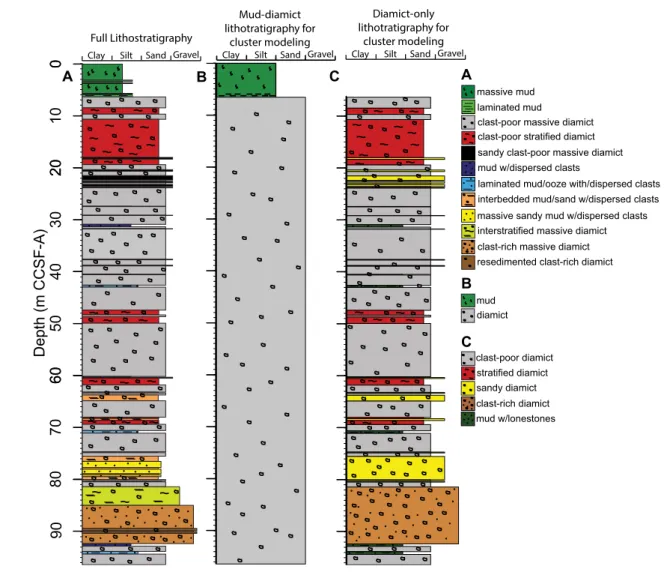
We use these 12 lithofacies to generate a lithostratigraphic section at cm-scale resolution for the composite Site U1419 record (Fig. 5A). For ease of comparison with our other data sets and cluster analysis testing,

we condense this high-resolution record into a bimodal mud and diamict lithostratigraphy (Fig. 5B) and a diamict-only lithofacies (Fig. 5C). For the bimodal mud-diamict lithofacies section, any lithofacies that contain clasts are grouped into a general diamict facies, and those lacking lonestones are grouped into a general mud facies (Table 2). The mud lithofacies represents 7% of the composite splice, while the diamict portion is 93% of the core (Table 3). P CT Clast-poor diamict B P CT Stratified diamict D A Massive mud CT P Clast-rich diamict CT P F Sandy diamict CT P E

Mud w/dispersed clasts

P CT

C

5c

m

Figure 4. Lithofacies identified within U1419 from core photographs and computed tomography (CT) images of U-channels collected from the core. A–F depicts a section of core photograph (P) and its corresponding com-puted tomography (CT) image. Comcom-puted tomography images are used to highlight changes in density (lighter = more dense; darker = less dense), and lonestones (clasts) that are not visible in core images. Note scale bar in (A).

Research Paper

7

Penkr

ot et al.

| IODP Site U1419

GEOSPHERE

| Volume 14 | Number 4

TABLE 1. OBSERVED LITHOFACIES IN U1419

Lithofacies Code Description Core Photograph CT Scan

Massive mud Fm Fine-grained, structureless, silt and clay._{Bioturbated w/some burrows preserved 5 cm}

Laminated mud Fl Mud/silt laminae

Clast-poor

massive diamict Dmm

1-5% clasts floating in mud matrix. Poorly sorted. Denser clasts appear lighter in computed

tomography (CT) imagery.

Clast-poor

stratified diamict Dms

1-5% clasts floating in mud matrix w/low density, fine-grained stratifications that

range from a few mm to ~1 cm thick. Stratification contacts appear diffuse.

Sandy clast-poor massive diamict sDmm

1-5% clasts floating in sandy mud matrix. Poorly sorted. Has higher density than surrounding diamict. Tends to have sharp lower contact

and gradational upper contact.

Mud/ooze with dispersed clasts Fdo

Fine-grained, structureless, silt and clay. Green colored, with abundant

diatoms and few (<1%) clasts

Research Paper

8

Penkr

ot et al.

| IODP Site U1419

GEOSPHERE

| Volume 14 | Number 4

TABLE 1. OBSERVED LITHOFACIES IN U1419 (continued)

Lithofacies Code Description Core Photograph CT Scan

Laminated mud/ooze with

dispersed clasts Flo Mud/silt laminae with few (<1%) clasts

Interbedded mud/sand with

dispersed clasts F/Sd

Interbedded mud and fine sand. Sand layers have sharp bottom contact and gradational upper contact with few (<1%) clasts

Massive sandy mud with

dispersed clasts mFSd

Bioturbated mud and fine sand with few (<1%) clasts

Interstratified

massive diamict DmmIS

Intervals of clast-poor diamict (1-5% clasts) interstratified with intervals of clast-rich diamict (>5% clasts) and silt stringers. Clast rich interval vary in thickness from 3 cm to ~20 cm.

Clast-rich

massive diamict DmmCr >5% clasts floating in mud matrix

Resedimented

clast-rich diamict rDmmCr

>5% clasts floating in mud matrix with evidence of displacement

Research Paper

9

GEOSPHERE| Volume 14 | Number 4

We further subdivide the diamict portion of the lithostratigraphy at a verti cal scale that allows for testing of whether the subtle, finer vertical-scale lithofacies can be identified using cluster analysis of downcore logging data. We focus on the diamict interval because diamict facies comprise a majority of the spliced section and contain ten out of the 12 visually observed litho-facies. In addition, the diamict facies likely contain much of the information on spatial variations in glacier extent (e.g., Cowan et al., 1997). We combine the ten clast-bearing lithofacies into five simplified lithofacies based on tex-ture and concentration of lonestones (clasts)—clast-poor massive diamict,

clast-poor stratified diamict, clast-poor sandy diamict, clast-rich diamict, and mud with lonestones, creating a diamict-only lithofacies (Table 4; Figs. 4B–4F and 5C).

Many of the ten clast-bearing lithofacies display fairly similar logging prop-erties (Fig. 6; Fig. S1 [footnote 1]), and combining the most texturally similar facies allows for greater differentiation of the facies that are modeled through classification analysis. The facies that are condensed into overarching groups vary subtly, often by features not easily identified by the logging data (e.g., bioturbation), and they are interpreted to be deposited under similar glacier

Clay Silt Sand Gravel

Full Lithostratigraphy

Clay Silt Sand Gravel

Mud-diamict lithotratigraphy for cluster modeling Diamict-only lithotratigraphy for cluster modeling

Clay Silt Sand Gravel

A

B

C

laminated mud/ooze with/dispersed clasts interbedded mud/sand w/dispersed clasts laminated mud

sandy clast-poor massive diamict clast-poor stratified diamict

interstratified massive diamict clast-poor massive diamict

clast-rich massive diamict massive mud

mud w/dispersed clasts

C

B

A

80

60

40

20

0

Depth (m CCSF-A)

70

60

50

30

20

10

0

90

resedimented clast-rich diamict massive sandy mud w/dispersed clasts

Figure 5. Lithostratigraphy of spliced composite from Site U1419. (A) Full litho-stratigraphic section containing all facies; (B) simplified mud-diamict lithostratig-raphy; (C) diamict-only lithostratigraphy. Simplified lithostratigraphy is created for ease of comparison with cluster analyses results. Core depth is plotted in meters of core composite depth below sea floor, method A (CCSF-A) (Jaeger et al., 2014).

Research Paper

10

GEOSPHERE| Volume 14 | Number 4

conditions. Additionally, some of these facies are only seen within very small intervals a few cm thick (i.e., sandy clast-poor diamict), which alone would be aliased by the resolution of the logging properties, which range from 2 to 10 cm.

Downcore Logging Data

The downcore logging data resolve core properties at a range of vertical scales that generally correspond with lithostratigraphy (Fig. 7). Sediment color reflectance (b*) and MS appear to generally be inversely correlated, with high-est b* and lowhigh-est MS values occurring from 0–6.32 m CCSF-A, and the low-est b* and highlow-est MS from 6.32–96.64 m CCSF-A. In the lower interval, sev-eral peaks in b* occur, with values similar to those found in the upper 6.32 m CCSF-A of core. Natural gamma radiation values mirror MS with the lowest values found in the upper 6.32 m CCSF-A, with higher and relatively consistent values observed below.

Aluminum and Si generally covary with average values increasing down-core. Both K and Rb show highest values in the upper 6.32 m CCSF-A of the core and appear to be correlated. A major low in K is observed between 83.2 and 91.4 m CCSF-A that is not seen in Rb. Calcium displays the most down-core variability of any of the elements and appears to roughly correlate with MS below 6.32 m CCSF-A. Average Ca concentrations decrease toward the bottom of the composite splice, with the most variability observed between 80.7 and 94.4  m CCSF-A. Zirconium is roughly inversely correlated with K and Rb, with values showing a stepwise increase at 6.32 m CCSF-A, and then steadily decreases until 73.6  m CCSF-A. Between 73.6 and 80.9  m CCSF-A, Zr displays high variability, and at 80.9 m CCSF-A, Zr displays a stepwise de-crease in values.

Logging Properties of Lithofacies

To relate changes in logging properties with visually observed lithofacies, we compare the standardized (z-score) value of each logging property to the lithofacies (Fig. 6). The median and interquartile ranges of z-scores are calcu-lated for each logging parameter within each lithofacies (File S2 [footnote 1]). Logging properties having positive median z-score values are relatively en-riched, and those with negative values are relatively depleted, with the abso-lute value a measure of the degree of deviation from the mean of that property for the entire analyzed section (i.e., a value of +1 indicates enrichment at 1σ).

For the bimodal mud-diamict lithostratigraphic grouping (Figs. 6A and 6B), the diamict facies has nearly average concentrations of all the logging proper-ties (i.e., value ~0). In contrast, the mud facies is average for Zr, very enriched (~+2σ) in b* (very green) and Rb, moderately enriched (~+1σ) in Ca and K, moderately (~–1σ) depleted in Al and Si, and very depleted (~–2σ) in NGR and MS (Table 4). Because diamict is 93% of the total described section (Table 3), TABLE 2. MUD-DIAMICT LITHOSTRATIGRPAHY FACIES

Lithofacies Codes Description

Mud Fm, Fl No lonestones or obvious glacial input present; green mud, massive and laminated. Diamict Dmm, Dms, sDmm, F/Sd, mFSd, DmmCr,

DmmIS, rDmmCR, Fdo, Flo Few to abundant lonestones present throughout. Ranging from massive to stratified tolaminated with some laminated and massive sandy intervals.

TABLE 3. DISTRIBUTION OF LITHOFACIES OBSERVED IN U1419 Lithology Thickness(m) Length(%) Mud-diamict lithostratigraphy Mud 7.56 7.8 Diamict 89.08 92.2 Diamict-only lithostratigraphy Massive diamict 56.13 62.2 Stratified diamict 13.25 14.7 Mud with lonestones 2.72 3.0

Sandy diamict 9.46 10.5

Clast-rich diamict 8.76 9.7

TABLE 4. DIAMICT-ONLY LITHOSTRATIGRAPHY FACIES

Lithofacies Codes Description

Clast-poor massive diamict Dmm 1%–5% clasts floating in mud matrix. Poorly sorted.

Clast-poor stratified diamict Dms 1%–5% clasts floating in mud matrix with low-density, fine-grained stratifications that range from a few mm to ~1 cm thick. Poorly sorted. Stratification contacts appear diffuse.

Clast-poor sandy diamict sDmm, F/Sd, mFSd Sandy, relatively high density. Clast-rich diamict DmmCr, DmmIS, rDmmCr >5% clasts floating in mud matrix.

Research Paper

11

GEOSPHERE| Volume 14 | Number 4

it is understandable its logging properties have standardized values close to zero; whereas the mud lithofacies displays greater variability.

For the diamict-only lithostratigraphic grouping, there is more variability in the range of standardized logging values within each sublithofacies. In this diamict-only interval, clast-rich diamict is the dominant lithofacies, represent-ing 62.2% of the core, while stratified diamict makes up 14.7%, sandy diamict 10.5%, clast-rich diamict 9.7%, and mud with lonestones 3.0% (Table 3). Clast-poor diamicts have a comparatively average composition with slight

enrich-ment in Al, K, and Si and slight depletion of Rb, Ca, and Zr (Fig. 6C). Stratified diamicts are defined by moderately enriched K, Rb, and Zr (~+0.5σ) and mod-erately depleted Si, MS, and NGR (~–0.5σ). Both sandy and clast-rich diamicts are compositionally similar, being moderately depleted in b*, Al, K, Rb, and Ca. However, sandy diamict is moderately enriched in Zr, while clast-rich diamict is moderately enriched in Si, moderately depleted in Al, and very depleted in K. Mud with lonestones is moderately enriched in b*, NGR, Si, and Ca, and moderately depleted in Al and Zr.

Principal Components

For the unsupervised cluster analysis, we reduce multivariate space by using only the first three principal components (PC). Regardless of samples or input parameters used in the factor model, PC1 represents 38%–54% of the variability, PC2 25%–34%, and PC3 15%–28%, with the three overall representing 90%–100% of the total variance (Fig. 8). Physical properties (b*, MS, and NGR) appear most useful for delineating variations in composition (b* and MS) and clay content (NGR). Elemental data appear to best capture differences in sand versus clay content (Ca, Zr, and Si versus K, Rb, and Al) and composition (Ca and Si).

Mud-Diamict Lithostratigraphy

For data groups G1 and G2, PCs 1 and 2 are dominated by parameters that tend to follow the relative parameter importance shown in Figure 6A. Mag-netic susceptibility, NGR, and b* values dominate the variance explained by PC1 and PC2 (Figs. 8A and 8B), suggesting that these PCs reflect the relative difference in grain size and composition between the mud and diamict litho-facies. For the element-only data group G3, there is a greater variability on the composition of each PC (Fig. 8C). PC1 of G3 is largely influenced by Al and Si, which are both moderately depleted in the massive mud facies (Fig. 6A). For PC2, Ca, Si, and Zr group together and may represent a sandier component; whereas Al, Rb, and K group together and may represent a muddier compo-nent. PC3 is mostly represented by Ca alone, and may represent a nontextural (i.e., biogenic) Ca component.

Diamict-Only Lithostratigraphy

For data groups G1 and G2, PC1 is dominated by NGR and b* (Figs. 8D and 8E), suggesting its variance is explained by differences in grain size and com-position. Magnetic susceptibility is the dominant variable for PC2 in G1 and PC3 in G2, and may represent a difference in sediment composition. PC3 in G1 and PC2 in G2 are mainly influenced by a b* and NGR grouping, representing a muddy, greener, diatom-bearing component. For G3, an Al and K versus Zr grouping dominates PC1, suggesting it represents a muddier versus coarser

Mud-Diamict Lithostratigraphy Diamict-Only Lithostratigraphy b* NGRMS Al K Rb Si Ca Zr −2 02 4 Mud b* NGRMS Al K Rb Si Ca Zr −2 −1 012 Diamict

Standardized Concentration (no units)

b* NGRMS Al K Rb Si Ca Zr −2 −1 0123 Stratified diamict b* NGRMS Al K Rb Si Ca Zr −3 −2 −1 0123

4 Sandy clast-poor diamict

b* NGRMS Al K Rb Si Ca Zr −2 −1 01 2 Clast−poor diamict b* NGRMS Al K Rb Si Ca Zr −2 −1 012

Mud with lonestones b* NGRMS Al K Rb Si Ca Zr −3 −2 −1 01 2 Clast−rich diamict

Standardized Concentration (no units)

A

B

C

D

F

E

G

that are standardized (z-score) for all obser-vations and grouped by lithofacies in which they occur. Lithofacies are simplified groups as shown in Figure 5. Positive z-score val-ues are relatively enriched while those with negative values are relatively depleted. Degree of enrichment and/or depletion re-flected in absolute value, representing one to four sigma deviation from the mean.

Research Paper

12

GEOSPHERE| Volume 14 | Number 4

variant (Fig. 8F). Silicon, possibly representing a sand component, largely con-trols PC2. PC3 is predominately influenced by Ca but not with Si, suggesting it is representing biogenic Ca rather than Ca-rich plagioclase.

Supervised Classification Model Results

Quadratic discriminant analysis and SVM model results differ greatly in ac-curacy between the simpler mud-diamict lithostratigraphy and the more com-plex diamict-only lithostratigraphy. For the mud-diamict case, both QDA and SVM models are 100% accurate with a Cohen’s Kappa value of 1. The Kappa statistic is a metric that compares an observed accuracy with an expected

ac-curacy given the relative abundance of that group or lithofacies (Fleiss et al., 2013). It is a more accurate measure of model performance when there is a strong imbalance in the number of observations in a particular class (e.g., diamict). In decreasing order of importance in the accuracy of the models are NGR, Rb, b*, Al, Si, MS, and Ca (File S1 [footnote 1]).

Neither supervised modeling approach is accurate with the diamict-only lithofacies. The Greedy Wilks analysis identified Si and Zr as the parameters that explained most of the variance in the diamict-only data set (File S1 [foot-note 1]). The QDA model is only 44% accurate (Kappa = 0.21), and the SVM model is 42% accurate (Kappa = 0.22). In general, both models struggle with the nonmassive diamict facies; they successfully classify massive diamict cor-b*

A

B

C

D

E

F

G

H

I

J

Clay Silt Sand Gravel

80 60 40 20 0 Depth (m CCSF-A) 70 60 50 30 20 10 0 90 stratified diamict sandy diamict clast-poor diamict clast-rich diamict mud w/lonestones massive mud _{−5.0 −2.5 0.0 2.5 5.0} Vol. norm. MS (cm3_/g) 25 50 75 100 125 .02 .025 .03 .035 Vol. norm. NGR (cps/g) 8 10 12 14 % Al (nms) .5 1.0 1.5 2.0 % K (nms) 2 4 6 % Ca (nms) 30 40 50 % Si (nms) 20 30 40 50 60 70 Rb ppm (nms) 20 40 60 80 Zr ppm (nms)

Figure 7. Logging data used in cluster models plotted on core composite depth below sea floor, method A (CCSF-A). (A) Simplified lithostratigraphy; (B) shipboard b* color reflectance; (C and D) volume-normalized magnetic susceptibility and natural gamma-ray activity, from Walczak et al. (2015); (E–J) scanning XRF elemental data calibrated using the normalized median-scaled method (NMS; Lyle et al., 2012).

Research Paper

13

GEOSPHERE| Volume 14 | Number 4

rectly but also tend to classify the other lithofacies as massive diamict (File S1 [footnote 1]). In these models, the relative importance of parameters varies for each lithofacies, with b*, Si, and Al being relatively the most important in successfully distinguishing between the lithofacies groups.

Unsupervised Clustering Model Results

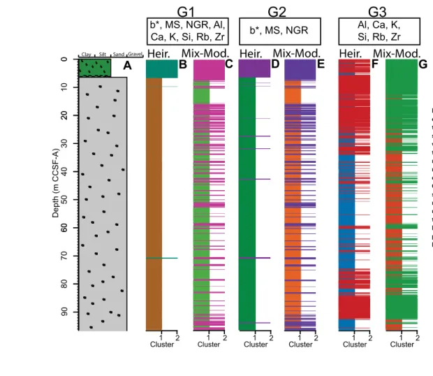
Clustering using the hierarchical and modified-mixture model techniques results in highly variable cluster lithologies that depend on the clustering rou-tine and input data used (Figs. 9 and 10). A total of 12 cluster-based litholo-gies are produced—one for each of the input data groups (G1, G2, and G3) and clustering routine (hierarchical and modified-mixture model), for both the mud-diamict and diamict-only lithostratigraphies. Note that the cluster

identi-fier (e.g., cluster 4), is arbitrarily set by the analysis code and is not consistently associated with a particular cluster-based lithology. For this study, we renamed the clusters in rank order so that cluster 1 indicates the most common cluster and Cluster 5 the least common.

Mud-Diamict Lithostratigraphy

Modeled cluster groupings have varying degrees of similarity with the ob-served mud-diamict lithostratigraphy. Although each clustering approach can create more than two cluster groups, for this first scenario, we limited models to two clusters to best compare with the bimodal mud-diamict lithostratigra-phy. We compare the clustering results with the observed lithofacies by com-paring the z-score of the variables within each cluster to those of the observed

−4−2 0 2 PC 1 −3 −1 0 1 3PC 2 −2 PC 30 2−0.5 0.5PC 1 −0.5PC 20.5 −0.5 0.5PC 3

Mud-Diamict Lithostratigraphy

B

Principal Component Score

0% 57% AlCaRbZrK Si b* NGR MS PC1 83% Al CaRbZrKSi b* NGR MS PC2 98% AlCaRb_ZrKSi b*NGR MS PC3 −1 −0.5 0 +0.5 +1 G1

A

Principal Component Loadin

g 0% 40% Al CaRb Zr K Si PC1 72% Al Ca Rb Zr K Si PC2 90% Al Ca RbZr K Si PC3 −1 −0.5 0 +0.5 +1 G3

C

Figure 8 (on this and following page). Ro-bust principle component analyses (Templ et  al., 2011) of logging data divided into three groups: G1—physical properties and elemental data inputs; G2—physical prop-erties only; G3—elemental data only. Prior to principal component analysis (PCA) analysis, magnetic susceptibility (MS), natural gamma radiation (NGR), and b* values are standardized; elemental data are isometric log ratio (ilr) transformed (Templ et  al., 2008); (A–C) data for en-tire spliced composite record; (D–F) data for diamict-only section. The first three components represent 90%–100% of the total variance and are used in subsequent cluster analyses. Depth scale is same as Figure 7.

Research Paper

14

GEOSPHERE| Volume 14 | Number 4

lithofacies. This helps identify which cluster is most similar to the lithofacies we are attempting to model (Fig. 11 and Fig. S2 [footnote 1]).

Data groups G1 and G2 have similar cluster modeling results (Fig. 9). Both the hierarchical and mixture-model clustering results contain a cluster that is related to the mud lithofacies. This cluster contains enriched b*, K, Rb, and Ca, and depleted NGR, MS, and Si values that are indicative of the greener, fine-grained mud lithofacies. The second cluster is composed of average physical property values and elemental concentrations that represent the volumetri-cally dominant diamict facies. Both clustering routines show similar logging property enrichment and depletion patterns within the clusters for G1 and G2. However, the hierarchical clustering routine reveals more highly enriched or more highly depleted logging properties, while the mixture-model clustering results show only moderately enriched or moderately depleted properties (Fig. S2 [footnote 1]).

G3 cluster results differ greatly from G1 and G2. There is no cluster for this model that definitively represents the distinctive mud facies (i.e., enriched b*, K, Rb, and Ca and depleted NGR, MS, and Si) (Fig. 9; Fig. S2 [footnote 1]). Both hierarchical and mixture-model cluster results contain similar variations in logging properties, with one cluster containing moderately enriched Al, moderately depleted Zr, and nearly average values for all other logging prop-erties. Logging properties of the second cluster are opposite, with moderately enriched Zr, moderately depleted Al, and nearly average for all other variables.

We observe that the vertical heterogeneity of the logging data produces varying amounts of vertical detail represented by each cluster group. Data groups G1 and G2, which contain physical property logging data, have less downcore variability between clusters than G3, which only utilizes the scan-ning XRF elemental data. This is illustrated by the fact that G1 and G2 cluster lithologies have one cluster that comprises the top 6.32 m CCSF-A core (mud

0% 42% AlCaRbZrKSi b* NGR MS PC1 73% Al CaRbZrKSi b* NGR MS PC2 98% AlCaRb_ZrKSi b* NGR MS PC3 −1 −0.5 0 +0.5 +1 G1 0% 52% b* NGR MS PC1 79% b* NGR MS PC2 100% b* NGR MS PC3 −1 −0.5 0 +0.5 +1 G2 0% 38% Al Ca Rb Zr K Si PC1 72% Al Ca Rb Zr K Si PC2 91% Al Ca Rb ZrK Si PC3 −1 −0.5 0 +0.5 +1 G3 −2 0 2 PC 2 −2−10 1 2 3 PC 1 -3 -1 0 2PC 3 −2 0PC 12−2 0PC 22 −2 0 2 PC 3 −0.4 0.4 0.8PC 1 −0.5 0.5PC 2 −0.3 0 0.2PC 3

D

E

F

Principal Component Score

Principal Component Loading

80 60 40 20 Depth (m CCSF-A) ₇₀60 50 30 20 10 90 -2 1 Figure 8 (continued).

Research Paper

15

GEOSPHERE| Volume 14 | Number 4

portion of the core), with the second cluster dominating the portion of the core below 6.32 m CCSF-A (diamict portion of the core). For G3, there is no single cluster that describes the entire top 6.32 m CCSF-A of core, and the section of core below 6.32 m CCSF-A frequently alternates between clusters. The difference in downcore cluster variance also is evident in the percent-age of core contained in the dominant cluster (Table 5). There is little dif-ference between G1 and G2 for the percentage of core section represented by the dominant and minor cluster. Within each data group (G1–G3), the model-based clustering approach has more downcore variability than hier-archical clustering (Fig. 9). This is also evident in the cluster percentages, where the difference between the two cluster lengths is greater for the G1 hierarchical clusters (92% versus 8%) than the G1 mixture-model clusters (76% versus 24%; Table 5).

Diamict-Only Lithostratigraphy

We suggest that cluster modeling can better resolve the heterolithic nature of this site if the number of clusters is increased to reflect the increased number of lithofacies and by limiting the input data to only the diamict portion of the core. As with the mud-diamict lithostratigraphy, we chose to limit the number of cluster groups to match the number of end-member lithologies we are trying to model (five). The same three data groups (G1–G3) are used for modeling the diamict-only lithostratigraphy. To identify which cluster is most similar to each observed lithofacies, the z-score of each logging property within each cluster again is compared to the observed diamict lithofacies (Fig. S3 [footnote 1]).

As expected, diamict-only lithostratigraphy modeling results are vertically more complex than those for the mud-diamict lithostratigraphy (Fig. 10). The

Clay Silt Sand Gravel

Heir. Mix-Mod. Heir.

Heir.

G1

G2

b*, MS, NGR

G3

Cluster1 2 Cluster1 2 Cluster1 2 Cluster1 2 Cluster1 2 Cluster1 2

Mix-Mod.

Mix-Mod.

A

B

C

D

E

F

G

Al, Ca, K,

Si, Rb, Zr

b*, MS, NGR, Al,

Ca, K, Si, Rb, Zr

Figure 9. Cluster modeling results for prin-cipal component analysis (PCA) scores for three data groups for the mud-diamict simplified lithostratigraphy. To compare with bimodal lithofacies, only two clus-ters are modeled using hierarchical and mixture-model clustering. Cluster 1 rep-resents the most common cluster and cluster 2, the least common (Table 5). Clusters do not necessarily relate to an ob-served lithofacies or to a cluster in another model. Statistical measures used to eval-uate the fit between cluster results and the observed lithology (Table 7) indicate hierarchical modeling of the G1 data set provides the closest match to observed lithofacies.

Research Paper

16

GEOSPHERE| Volume 14 | Number 4

most common cluster from each model result contains relatively average log-ging properties common to the observed clast-poor diamict that dominates this interval of core (Table 5; Fig. S3 [footnote 1]). However, the remaining clusters do not contain logging property associations that can be associated with the observed lithofacies (Fig. 6). Cluster groups for G1 and G2 hierarchical clustering and G3 hierarchical and mixture-model clustering are nearly iden-tical; while G1 and G2 mixture-model clustering results are distinct (Fig. 10).

DISCUSSION

Our results indicate that it is possible to use supervised and unsupervised machine learning models on physical and elemental core logging data to clas-sify glacimarine lithofacies with varying success. Bimodal mud-diamict

litho-facies interpreted as nonglacial versus glacial conditions can be successfully identified using physical properties data augmented with scanning XRF analy-ses. In both QDA and SVM supervised classification models, the combination of these parameters resulted in high accuracy. For unsupervised cluster analy-sis, the inclusion of scanning XRF elemental abundance with physical property data offers only a slight improvement in model success. For the heterolithic diamict-only glacimarine lithofacies that are interpreted to represent variations in glacier extent, all modeling approaches are less successful; although un-super vised cluster analyses provided slightly better accuracy.

Supervised classification analysis is most useful for discerning between lithofacies when the number and types of facies expected is known. When using classification analysis as an alternative to CT scans and/or X-radio-graphs to highlight subtle lithofacies variations, unsupervised cluster analysis

Clay Silt Sand Gravel

1 2 3 4 5 Cluster 1 2 3 4 5

Cluster 1 2 3 4 5Cluster 1 2 3 4 5Cluster 1 2 3 4 5Cluster

Heir.

Heir.

Mix-Mod.

Heir.

Mix-Mod.

G1

G2

G3

A

B

C

D

E

F

G

b*, MS, NGR, Al,

Ca, K, Si, Rb, Zr

b*, MS, NGR

Al, Ca, K,

Si, Rb, Zr

Mix-Mod.

Figure 10. Cluster modeling results for principal component analysis (PCA) scores for three data groups for the diamict-only lithostratigraphy. To compare with litho-facies, only five clusters are modeled using hierarchical and mixture-model clustering. Clusters are presented in rank order, with cluster 1 representing the most common cluster in each model and cluster 5 the least common (Table 5). For each model, cluster 1 is colored gray and is comparable to the clast-poor diamict lithofacies. The other clusters do not necessarily relate to a lithology or are comparable between models. Statistical measures used to eval-uate the fit between cluster results and the observed lithology (Table 7) indicate overall poor correspondence between the two. Mixture modeling of the G3 data set provides the closest match to observed lithofacies, but only weakly.

Research Paper

17

GEOSPHERE| Volume 14 | Number 4

is prefera ble because it does not constrain the model to already known facies. The following discussion will primarily focus on interpretation of the unsuper-vised cluster models, which offers the opportunity to provide new information from the natural clustering of the logging data. We contend that the unsuper-vised cluster modeling results serve as a valuable complementary data set alongside visual observations and imaging for lithofacies coding, rather than as a replacement for a visual core description and CT scan and/or X-radiograph imaging. When cluster-model results are compared to observed lithostratigra-phy and downcore plots of elemental ratios, a basic record of glacial dynamics can be discerned.

Evaluation of Classification Approaches

Both supervised and unsupervised classification approaches were most ac-curate with the bimodal lithofacies grouping but were less so when applied to the diamict-only interval. Quadratic discriminant analysis and SVM performed the most accurate classification without misclassification for the bimodal litho-facies, followed by hierarchical clustering. These three approaches offered the most accurate and interpretable results for the mud-diamict models presented in this study; whereas either classification approach used for the diamict-only

models had little influence on the results, with no model able to accurately pre-dict the diamict-only lithofacies. Unsupervised mixture-model clustering does not perform well when differentiating between clusters with uneven number of observations, such as those in the mud-diamict lithostratigraphy (Table 3; Ertöz et al., 2003). While the clusters within the diamict-only section are not completely even, they are more so than the mud-diamict clusters, and so the mixture-model clustering performed as well as hierarchical clustering. Overall, choice of input data had a greater impact on the clustering results than the clustering routine.

When using hierarchical clustering, choosing the appropriate number of clusters is critical to model performance, and with little to no a priori informa-tion on lithofacies, it is difficult to constrain the appropriate numbers of clusters (Milligan and Cooper, 1985). However, if the number of expected lithofacies within a model can be constrained, hierarchical clustering becomes more use-ful. When the number of clusters is unknown, mixture-model clustering may be a better choice, because the Bayesian information criterion (BIC) can be useful for informing on an appropriate number of clusters to select (Fraley and Raftery, 1998; Raftery and Dean, 2006). Plots of BIC values for models used in this study show that our choice of using two and five clusters for our mud-diamict and diamict-only lithostratigraphy modeling is appropriate (Fig. S4 [footnote 1]).

Clay Silt Sand Gravel

Cluster1 2 Heirarchical clustering b*, MS, NRG, Al, K, Rb

Si, Ca, Zr

Visually Observed Lithofacies Modeled Lithofacies Clusters

Establishing cluster lithology

Diamict Mud Cluster 2 Cluster 1 Observed Lithology Cluster Lithology Diamict −2 −1 01 2 Cluster 1 Mud −2 01 2 _{Cluster 2} b* NGRMS Al K Rb Si Ca Zr b*NGRMSAl K Rb Si Ca Zr 80 60 40 20 0 Depth (m CCSF-A) 70 60 50 30 20 10 0 90 80 60 40 20 0 Depth (m CCSF-A) 70 60 50 30 20 10 0 90

Figure 11. Workflow relating cluster results to lithofacies. Box-whisker plots for logging data within each cluster group is related to data from each lithofacies. The cluster having the closest visual correspondence between plots is then associated with that lithofacies (e.g., cluster 2 with mud), and a cluster lithology is created.

Research Paper

18

GEOSPHERE| Volume 14 | Number 4

Evaluation of Model Input Data

Physical property logging data are best at capturing end-member lith-ologies, such as mud and diamict. This is because the greatest variation in physical properties between lithofacies is observed at the end-member scale (Figs. 3 and 6). The measurement resolution of the physical prop-erty logging data is too low to resolve thin beds of alternating lithofacies and only captures thicker major facies. Magnetic susceptibility and NGR measurements represent an average of an 8  cm and 10  cm interval, re-spectively; while b* and the scanning XRF elemental data are point mea-surements collected every 2 cm (Jaeger et al., 2014; Penkrot et al., 2017a). Some lithofacies within Site U1419 contain beds that are relatively thin— approximately a few cm (i.e., sandy diamicts) to 10–20 cm (i.e., mud with dispersed clasts). These facies are poorly resolved over the 8–10  cm of core that are integrated by the MS and NGR measurements, which con-fines the usefulness of our MS and NGR data sets to simple, end-member lithostratigraphies where beds occur on the meter scale rather than the cm scale. Cross plots of MS versus b* plotted by observed lithology illustrate the ability of the physical properties to better distinguish between the bi-modal mud-diamict lithofacies than the heterogeneous diamict-only litho-facies (Fig. S5 [footnote 1]).

Scanning XRF elemental data are most useful in identifying subtle vari-ations in sediment composition and texture that occur between lithofacies. Proxies for both coarse (Zr and Si) and fine-grained (Al, K, and Rb) minerals are represented in the elemental data. Out of the three shipboard-measured properties utilized in this study, NGR is the only one able to capture changes in grain size as a proxy for the relative amount of clay minerals. Lithofacies variations within the diamict-only section are primarily defined by differences in the amount of coarse grains (i.e., clast-rich diamict versus clast-poor diamict versus mud with lonestones); thus the elemental proxies for coarse grains pro-vide more distinguishing power than NGR.

Inclusion of MS, NGR, and b* with elemental data for diamict-only classifi-cation did not improve overall accuracy for any method. In cluster analysis, it did not create a more accurate model of cluster lithology due to high loading scores of the physical properties that may overweight their importance com-pared to the elemental data (Figs. 8A and 8D). We recognize that this is caused by using standardized values for physical properties and log-ratio values for elemental data. However, when using mixed data treatment such as this, the resulting relationships between variables is not altered, and it is acceptable to combine both treatments into a single joint matrix prior to PCA analysis (Kynčlová et al., 2016). Both types of classification approaches for the diamict- only lithofacies that utilized b*, which has higher sampling resolution than MS and NGR, along with the elemental data, did not produce results that are able to accurately predict the observed lithofacies.

Evaluation of Cluster Model–Lithostratigraphy Relationships

Statistical measures are used to evaluate the fit between the unsupervised cluster model results and the observed lithology, while logging property distri-bution within each cluster allows for a textural and/or compositional interpre-tation to be made for the cluster. A Pearson’s chi-square test is used to test if the downcore position of cluster groups correspond with distinctive lithology categories, and Cramér’s V-value is used to test the strength of this relationship (Cramér, 1946; Liebetrau, 1983). Cramér’s V-value can vary from 0 to 1, with higher values indicating a higher association between cluster and observed lithofacies category.

Mud-Diamict Lithostratigraphy

Statistical evaluations for the six mud-diamict cluster models are found in Table 6. For all cluster models, a Pearson’s chi-square test results in a p value <<0.05, suggesting cluster modeling likely is able to capture the observed tran-TABLE 5. DISTRIBUTION (IN PERCENT) OF CLUSTERS WITHIN EACH CLUSTERING MODEL

Cluster

G1 G2 G3

Hierarchical Mixture-model Hierarchical Mixture-model Hierarchical Mixture-model Mud-diamict lithostratigraphy 1 92.0 23.9 8.6 76.4 65.7 60.1 2 7.9 76.1 91.4 23.6 34.3 39.9 Sum 100 100 100 100 100 100 Diamict-only lithostratigraphy 1 47.6 40.3 46.9 43.1 51.9 42.0 2 24.8 24.1 22.5 28.9 24.9 28.4 3 24.1 16.9 28.0 13.6 14.5 15.4 4 3.3 9.4 2.4 13.5 8.7 12.8 5 0.2 9.3 0.2 0.8 0.1 1.4 Sum 100 100 100 100 100 100