HAL Id: halshs-02482543
https://halshs.archives-ouvertes.fr/halshs-02482543v2
Preprint submitted on 6 Jul 2020
HAL is a multi-disciplinary open access
archive for the deposit and dissemination of
sci-entific research documents, whether they are
pub-lished or not. The documents may come from
teaching and research institutions in France or
L’archive ouverte pluridisciplinaire HAL, est
destinée au dépôt et à la diffusion de documents
scientifiques de niveau recherche, publiés ou non,
émanant des établissements d’enseignement et de
recherche français ou étrangers, des laboratoires
Human capital and welfare
Stefano Bosi, Carmen Camacho, David Desmarchelier
To cite this version:
Stefano Bosi, Carmen Camacho, David Desmarchelier. Human capital and welfare. 2020.
�halshs-02482543v2�
WORKING PAPER N° 2020 – 04
Human capital and welfare
Stefano Bosi
Carmen Camacho
David Desmarchelier
JEL Codes: I00, O11, C61
Human capital and welfare
∗
Stefano BOSI
†, Carmen CAMACHO
‡, David DESMARCHELIER
§June 10, 2020
Abstract
We introduce the Human Development Index (HDI) in a growth model à la Lucas (1988), where human capital has an additional positive effect on social welfare through the quality of individual health and education. In a simple economy with a Cobb-Douglas technology and logarithmic preferences, we provide the explicit trajectories for human capital, con-sumption and the HDI, which correspond to the Balanced Growth Path (BGP). Using a two-step maximization strategy, we compute the optimal initial value of the control variable, in this case, the initial optimal labor supply. In other words, we prove the optimality of the BGP. We high-light a HDI crossing property: the propensity to consume has a positive effect on the HDI in the short run, but negative in the long run. Finally, both the growth rate and overall welfare are proven to decrease in the propensity to consume.
JEL codes: I00, O11, C61.
Keywords: human capital, unbalanced growth, transversality condi-tion.
1
Introduction
When Mahbub ul Haq introduced human development as a compound process which included education and life expectancy, he paved the way for a new av-enue of research in development economics. The introduction of the Human Development Index (HDI) in ul Haq (1995) led to a new paradigm and to a modern theory of human development. However, although his works have influ-enced prominent economists like Amartia Sen, most growth theorists still focus on the utility of consumption. Stemming from the common belief that educated and healthy people enjoy life differently, the present paper considers that human capital is made of both education and health. Then we incorporate the HDI into the utility function defining a new composite good, which generalizes the
∗The authors acknowledge Cuong Le Van for his helpful comments and suggestions. †EPEE, University Paris-Saclay. E-mail: [email protected]. ‡PJSE UMR8545, PSE. E-mail: [email protected].
§BETA, University of Lorraine, AgroParisTech, CNRS, INRA. E-mail:
*Manuscript
consumption good. The new good embodies the notion that human capital is crucial to appreciate consumption, and it allows us to study the cross effect of human capital on the marginal utility of consumption.
While the seminal notion of human capital was introduced by Adam Smith in 1776 and later by Arthur Cecil Pigou in 1928, the modern theory of human capital can be traced back to Schultz (1961) and Becker (1964). Uzawa (1965) was first to incorporate human capital as an engine of growth in a theoretical model. The emergence of a new endogenous growth literature stimulated the interest of economists in the role of human capital. Building on Rosen (1976), Lucas (1988) underlined that the accumulation of human capital can trigger a mechanism of perpetual growth. In particular, he shows that the growth rate of income per capita depends on the growth rate of human capital, which in turn depends on the time individuals use to acquire skills and to protect their health. After Lucas (1988), the literature developed fast, scrutinizing all factors underlining the formation of human capital: education, transmission, health, culture,...1 Nevertheless, the literature becomes thinner regarding the other
various roles of human capital in an economy. Although sociologists report that as a matter of fact, education does affect life enjoyment, research in economics has for the most part neglected the role of human capital in welfare. Among the studies in sociology let us mention Ross and Wu (1995), who find that well educated individuals have a more fulfilling job and a better control over their lives. Moreover, they are in a healthier condition since they smoke and drink less. Similarly, Finkelstein et al. (2013) point out a complementarity between health and consumption demand: an increase of 1% in the number of chronic diseases reduces the marginal utility of consumption from 10% to 25%. From an economist’s viewpoint, this empirical evidence suggests that human capital does increase the marginal utility of consumption.
In order to consider the effect of education and health on wellbeing, it is necessary to enlarge the standard view of household’s preferences. Neverthe-less, introducing human capital in the utility function requires careful atten-tion. Indeed, from a theoretical perspective, the effects of human capital on the marginal utility of consumption are potentially ambiguous. On the one hand, human capital increases the marginal utility of consumption when, for instance, a well educated individual watches a movie and fully grasps all cul-tural references; on the other, human capital decreases the marginal utility of consumption when she becomes aware about the environmental damages of con-sumption. Empirical studies are not definite about the cross effect of human capital on consumption demand.
To our knowledge, Chakraborty and Gupta (2006) is the only model à la Lucas (1988) where human capital has the two essential roles we have underlined. There, human capital is, at the same time, a production factor and a source of wellbeing, and it enters both in the production and in the utility functions.
1Let us mention some of the most notorious works. Regarding education and human capital
formation, see De la Croix and Doepke (2003), Tamura (2001) or Cervellati and Sunde (2005). Concerning health and human capital formation, the interested reader can refer to De la Croix and Licandro (1999) or Kalemli-Ozcan et al. (2000).
When human capital affects more the agent’s preferences than consumption, then they find that the growth rate is higher along the Balanced Growth Path (BGP). When it affects less the production function, then multiple steady states coexist. Note however that the authors do not study the optimality of their BGP solution. Our objective is to address the important question of the role of human capital in wellbeing by considering a growth model where, as in Lucas (1988), the household chooses the working time and the time devoted to acquire skills. Following Ben-Porath (1967), there is no physical capital, but human capital affects both the production and the utility function as in Chakraborty and Gupta (2006).
Despite the absence of an optimality analysis in Chakraborty and Gupta (2006), intuition suggests that the optimality of the BGP is a relevant question when human capital enters preferences. Indeed, along the BGP, human capital grows at a constant rate by definition. Now, suppose human capital enters the utility function with standard properties, that is, a decreasing marginal utility. Then, depending on preferences, there may exist a critical level of human capital beyond which a further increase does not confer any extra utility. Beyond the threshold, the household stops acquiring skills and devotes all her time to work, in contradiction with the perpetual growth of human capital along a BGP. This paper aims precisely at questioning the optimality of the BGP when human capital is an argument of the utility function. Unlike Chakraborty and Gupta (2006), we reinterpret here the composite good as the mixture of consump-tion and human capital, in the form of a Human Development Index. Under a Cobb-Douglas technology and logarithmic preferences, we are able to provide the explicit trajectories for capital, consumption and HDI not only because we obtain the analytical solution to the system of differential equations, but also because we compute the initial control (labor supply) in a two-step maximiza-tion, which is new in growth literature. We actually prove that the optimal initial value of labor supply belongs to the BGP, demonstrating that the BGP is actually optimal from the start. Interestingly we highlight a HDI crossing property: the propensity to consume has a positive effect on consumption and, thus, on the HDI in the short run, but a negative effect in the long run. Finally, both the growth rate and welfare are proven to be decreasing in the propensity to consume, while, interestingly, the impact of time preference on welfare is positive when the initial human capital is below a threshold because of a scale effect.
The rest of the paper is organized as follows. The model is presented in Section 2. Section 3 considers the optimal solution when both utility and tech-nology are isoelastic functions. Assuming a unit elasticity of substitution both in preferences and in the HDI, Section 4 provides the explicit optimal solutions for human capital and consumption. Finally, Section 5 concludes. All the proofs are gathered in the Appendix.
2
The model
In the spirit of Chakraborty and Gupta (2006), we assume that human capital (health and education) increases workers’ productivity and households’ utility. There exists a representative household, who lives forever and maximizes the infinite-horizon utility:
max
! ∞
0
e−θtu (˜x (t)) dt (1)
choosing the optimal trajectories of consumption, c, and labor, l, and where the HDI2, ˜
x (t) ≡ x (c (t) , h (t)), is an increasing function of consumption and human capital. Optimal decisions are subject to the human capital accumulation law:
˙h (t)
h (t) ≤ B [1 − l (t)] (2)
the resource constraint:
c (t) ≤ y (t) ≡ h (t) l (t) (3)
and the initial condition h(0) ≡ h0. Output y (t) is a linear function of labor,
whose productivity is precisely human capital.
At each date in time, the representative household is endowed by one unit of time that she arbitrates between the working time in the firm, l (t) ∈ [0, 1], and the time spent to acquire skills, 1 − l (t). As in Lucas (1988), the growth rate of human capital is a linear function of 1 − l (t), and it attains its maximum value B when l(t) = 0, that is, when the household’s labor is zero.
For simplicity, we will omit the time argument in the following. Assumption 1 Function x : R2
+→ R+ is C2, strictly increasing and
homoge-neous of degree 1. u is C2, strictly increasing and strictly concave.
From (3) and the principle of non-satiation, c is uniquely determined by l for a given h. That is, the representative household chooses a unique control l to maximize her discounted intertemporal utility. In this context, an admissible control l is a locally integrable function l : [0, +∞) → [0, 1] satisfying (2) with h(0) ≡ h0> 0.
In order to solve the household’s program, let us introduce the Hamiltonian function:
H (h, l, λ, t) ≡ e−θtu (x (hl, h)) + λB (1 − l) h (4) The following proposition characterizes the optimal behavior of human cap-ital, h, and of µ ≡ λeθt, its shadow price.
Proposition 1 (necessary conditions) Consider program (1) under Assump-tion 1, and assume that there exists an interior continuous soluAssump-tion (l, h) ∈ [0, 1] × [0, +∞). Then, there exists a continuously differentiable function µ > 0
2
If y (t) ≡ h (t) l (t) denotes the per capita income (production) and c (t) = y (t), we recover ul Haq’s definition of HDI.
such that the optimal control l and the corresponding state variable h satisfy the following necessary conditions:
µ = u′(x) B ∂x ∂c (5) ˙µ µ = θ − B (1 − l) − u′(x) µ "∂x ∂cl + ∂x ∂h # (6) ˙h h = B (1 − l) (7) lim t→∞e −θtµh ∈ R (8)
Proof. See the Appendix.
Applying the implicit function theorem to the optimal condition (5), l can be written a function of h, that is l ≡ l∗(h, µ, t) ≡ ˜l∗(h). This observation
allows us to prove that the set of necessary conditions in Proposition 1 are not only necessary but also sufficient.3
Proposition 2 (sufficient conditions) Under Assumption 1, conditions (5) to (7) are necessary and sufficient optimal conditions for (1) if the Arrow-Kurz sufficient condition holds:
∂2x ∂c2 $ ˜ l∗(h) + h˜l∗′(h)% 2 + 2∂ 2x ∂c∂h $ ˜ l∗(h) + h˜l∗′(h)%+∂ 2x ∂h2 < 0 (9)
together with a stronger transversality condition: lim
t→∞e
−θtµ∗h∗= 0
Proof. See the Appendix.
Remark 3 The transversality condition limt→∞e−θtµ∗h∗∈ R is necessary for
optimality (see the proof of Proposition 1). Notice that limt→∞e−θtµ∗h∗ =
0 is a sufficient condition in Pontryagin et al. (2018, page 49) because the arrival space is not full-dimensional, which is not the case in our unconstrained problem. Many economic papers introduce limt→∞e−θtµ∗h∗= 0 as a sufficient
condition without giving proof, while few show the sufficiency (see Bosi et al., 2017, among others). Halkin was first to provide a mathematical example of a nonzero transversality condition, but meaningless in economic terms (see the footnote at page 46 in Arrow and Kurz, 1970, and the counterexample on page 271 in Halkin, 1974). Theorem 7.13 in Acemoglu (2009) demonstrates that the transversality condition is of the form limt→∞e−θtµ∗h∗= 0 when the economy
converges towards a steady state or towards a balanced growth path. We recover this property in the next section.
3The Arrow-Kurz sufficient conditions for optimality are not necessary and, in this sense,
they are possibly too restrictive: an optimal path can exist even if these conditions are not verified. See for instance Dechert and Nishimura, (1983), or Bambi and Gozzi (2019), where the first-order conditions lead to a unique optimal solution and the Arrow-Kurz conditions fail. However, we show in the following section that the Arrow-Kurz sufficient conditions are always verified in our problem when both u and x take isoelastic functional forms.
The following proposition provides the optimal trajectories for human capi-tal, labor supply and consumption demand.
Proposition 4 (dynamic system) The optimal solution (h, l)∗ satisfies the following dynamical system:
˙h h = B (1 − l) (10) ˙l l = θ − B − B∂x/∂h∂x/∂c− B (1 − l) $xu′′(x) u′(x) &c x ∂x ∂c+ h x ∂x ∂h ' +∂x/∂cc ∂∂c2x2 + h ∂x/∂c ∂2x ∂c∂h % c x ∂x ∂c xu′′(x) u′(x) + c ∂x/∂c ∂2x ∂c2 (11) where c = hl.
Proof. See the Appendix.
The computation of the optimal solution in the general case presented in Proposition 4 turns out to be impossible. However, in the case of isoelastic functional forms, the two-dimensional system (10)-(11) boils down to a single differential equation, easier to study.
3
The case of isoelastic functional forms
Consider the isoelastic functions:
u (x) ≡ ε ε − 1x ε−1 ε (12) x (c, h) ≡ (acσ−1σ + bhσ−1σ ) σ σ−1 (13) where ε is the (dynamic) elasticity of substitution between the HDI x today and tomorrow, and σ is the (static) elasticity of substitution in the HDI between the consumption c and the human capital h today.
Notice that there is no loss in generality if we assume
a + b = 1 (14) Indeed, if a + b )= 0, then ! ∞ 0 e−θt ε ε − 1 *( acσ−1σ + bhσ−1σ ) σ σ−1+ ε−1 ε dt = $(a + b)σ−1σ %ε−1 ε ! ∞ 0 e−θt ε ε − 1 *( ˜ acσ−1σ + ˜bhσ−1σ ) σ σ−1+ ε−1 ε dt where ˜ a ≡a + ba , ˜b ≡ b a + b, and ˜a + ˜b = 1
and, thus, arg max ! ∞ 0 e−θt ε ε − 1 *( acσ−1σ + bhσ−1σ ) σ σ−1+ ε−1 ε dt = arg max ! ∞ 0 e−θt ε ε − 1 *( ˜ acσ−1σ + ˜bhσ−1σ ) σ σ−1+ ε−1 ε dt
Proposition 5 (constant elasticities of substitution) If the utility func-tion and the HDI are defined by (12) and (13), then the Arrow-Kurz criterion (9) is satisfied. As a result, the first-order conditions (5) to (7) jointly with the transversality condition are necessary and sufficient for utility maximization. Optimal labor supply is driven by a single differential equation:
˙l = Bl " l + εb al 1 σ− 1 − εθ − B B # alσ−1σ + b alσ−1σ + bε σ ≡ ϕ (l) (15)
Proof. See the Appendix.
Proposition 6 (Balanced Growth Path) There exists a non-zero station-ary solution ¯l to (15), which is a solution to the following equation:
l + εb al
1
σ = 1 + εθ − B
B (16)
The steady state ¯l for labor supply determines the human capital growth rate g = B&1 − ¯l'. Furthermore, human capital and consumption grow at the same rate, that is, the economy follows a BGP:
¯
h (t) = eB(1−¯l)th0 (17)
¯
c (t) = eB(1−¯l)th0¯l (18)
The BGP in (17)-(18) is globally unstable. Proof. See the Appendix.
One of the main issues of this paper is the analysis of the impact of human capital on consumption demand. More precisely, we are interested in the impact of human capital on the marginal utility of consumption. As it follows from (13), this effect is negative (positive) if consumption and human capital are substitutes (complements). Hence, the elasticity of consumption-human capital substitution affects the optimal solution to the initial program, which generically differs from the BGP.
According to (15), labor supply l (t) decreases when the initial condition l0 < ¯l, and it increases otherwise. Note that the dynamics of labor are not
necessarily monotonic nor symmetric on either side of ¯l. l (t) can decrease to zero if l0< ¯l, while, if l0> ¯l, it reaches 1 in a finite lapse of time T . After date
The elasticity of consumption-human capital substitution, σ, affects the crit-ical value ¯l and, as such, it plays a key role in the dynamics of labor supply and human capital accumulation. Indeed, totally differentiating (16), we get
σ ¯ l ∂¯l ∂σ = B&1 − ¯l'+ ε (θ − B) σaB¯l + B&1 − ¯l'+ ε (θ − B)ln ¯l = εb¯l1σ σa¯l + εb¯l1σ ln ¯l < 0 Hence, σ has a clear negative impact on ¯l:
(1) the more substitutable are consumption and human capital, the lower is ¯l and, hence, the more likely is that l0 > ¯l. That is, the more plausible is
the situation in which labor supply increases over time until the critical date T beyond which the household stops investing in human capital;
(2) the less substitutable are consumption and human capital, the larger is ¯l. Thus, the more likely is that l0< ¯l, that is, the more plausible a decrease of labor supply to zero ensuring, asymptotically, the largest human capital (and consumption) growth rate g = B.
In other words, when human capital lowers the marginal utility of consump-tion (substitutability case), the individual no longer invests in human capital in the long run, or more precisely, beyond the critical date T . Conversely, when hu-man capital raises the marginal utility of consumption (complementarity case), the individual wants to invest in human capital at the maximal rate (B) in the long run.
For the sake of precision, let us observe that the optimal starting point l∗ 0
is endogenous. Consequently, even a very narrow (large) interval &0, ¯l' does not ensure that l∗0 > ¯l (neither that l∗0 < ¯l). In order to avoid any heuristic
interpretation and to determine unambiguously whether the optimal initial labor supply l∗
0is lower or higher than ¯l, in the following example, we fix σ = 1.
4
Optimal BGP in a simple economy
In order to obtain a complete description of the optimal solution, let us consider logarithmic preferences: u (x) ≡ ln x, with a Cobb-Douglas HDI: x (c, h) ≡ cαh1−α. These functions have unit elasticities of substitution: ε = σ = 1. Indeed, taking the limit of the logarithm of (13) and applying the de l’Hôpital’s rule, we get lim σ→1ln x (c, h) = σlim→1 ln(aeσ−1σ ln c+ beσ−1σ ln h ) σ−1 σ = a ln c + b ln h a + b = ln & cahb'
because a + b = 1 according to (13). Thus, x (c, h) = cahbin the limit. Setting α = a = 1 − b, we recover the Cobb-Douglas HDI function x (c, h) = cαh1−α.
In the Cobb-Douglas case, we are able to compute explicitly the optimal initial value for labor supply and to prove that the optimal initial value for labor supply (l∗0) is precisely αθ/B. This value corresponds to the BGP. In
other words, in the Cobb-Douglas case, the optimal trajectory is unique and coincides with the BGP.
To prove the optimality of the BGP, we adopt a constructive strategy based on the explicit solutions of the dynamic system. More precisely, following Borissov et al. (2018), we remaximize (1) with respect to l0 under the
sys-tem of constraints (10)-(11).
The following proposition provides the optimal paths for human capital and consumption demand depending on the value of α, B and θ.
Proposition 7 (optimal path) If ε = σ = 1, the optimal labor supply is given by l∗(t) = αθ/B and the optimal growth path is the BGP:
h∗(t) = h0e(B−αθ)t (19) c∗(t) = αθ Bh0e (B−αθ)t (20) ˜ x∗(t) = " αθ B #α h0e(B−αθ)t (21)
for any t ≥ 0. Along the BGP, the transversality condition is zero: lim
t→∞e
−θtµ (t) h (t) = e−θtµ∗ 0h0= 0
Proof. See the Appendix.
In light of Proposition 7, we can easily compute the impact of the three main parameters α, θ and B on the BGP in terms of the elasticities of h∗(t),
c∗(t), ˜x∗(t). Furthermore, their impact on the balanced growth rate and on the
welfare functional also obtain straightforwardly. Let us introduce the following critical dates:
Tx,α≡ 1 + ln l∗ θ , Tx,θ≡ 1 θ, Tc,α≡ 1 αθ, Tx,B≡ α B, Tc,B≡ 1 B
where l∗ = αθ/B is the optimal labor supply. We observe that Tx,α < Tx,θ <
Tc,α. Moreover, Tx,B< Tc,B and Tx,B< Tx,θ.
The following four corollaries directly stem from Proposition 7. Let us start by considering the effects of propensity to consume on the BGP.
Corollary 8 (propensity to consume) The impact of α on human capital is negative at any date. Its impact on consumption demand is positive in the short run, when t < Tc,α, and it becomes negative thereafter. Similarly, the impact of
α on the HDI is positive in the short run, while t < Tx,α(< Tc,α), and negative
in the long run, when t > Tx,α. Note that if Tx,α< t < Tc,α, the impact of α
is positive on consumption but negative on the HDI. In addition, the impact on the HDI is always negative if Tx,α< 0, that is if α < B/ (θe).
Proof. See the Appendix.
As Corollary underlines, α is a new important incoming parameter. When the HDI is given by (13) and σ = 1, the HDI is defined as a geometric average of income, which equals consumption, and human capital with weights α and 1 − α, respectively. Hence, α captures the propensity to consume by construc-tion, while 1 − α represents the propensity to invest in education and health. Consequently, the larger the propensity to consume, the higher the labor supply and the lower the capital accumulation at any time.
There exists a critical moment in time, Tc,α, such that the reaction of c∗
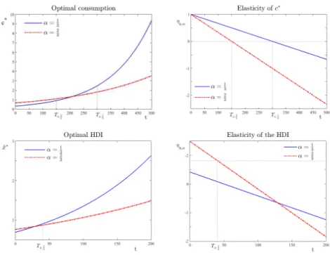
to α overturns. Indeed, in the short run, the higher labor supply increases consumption, while the lower human capital accumulation reduces both labor productivity and consumption in the long run. The following figures depict the crossing property plotting consumption demand and HDI for two different values of α, namely 1/3 and 2/3. For this exercise, h0 = 1, B = θ = 0.01
(quarterly discounting). The solid lines correspond to the lower propensity to consume, i.e. to α = 1/3. ηc,α and ηx,α respectively stand for the elasticity of c and x with respect to α.
Recall that the impact of α on the HDI is positive in the short run and negative in the long run if α > B/ (θe). Under our calibration this is the case when α = 1/3. However, α always affects negatively the HDI when α = 2/3. Here again, the higher labor supply increases consumption in the short run. In the long run, the lower human capital accumulation reduces both labor productivity and consumption.
Next, let us consider the effects of time preference on the BGP.
Corollary 9 (time preference) The impact θ on the human capital is nega-tive at any date. The impact on consumption is posinega-tive in the short run, when t < Tc,α, and negative thereafter. θ makes the HDI increase in the short run,
when t < Tx,θ, and decrease in the long run, when t > Tx,θ. Since Tx,θ< Tc,α,
if Tx,θ < t < Tc,α, then the impact of time preference is positive on consumption
but negative on the HDI. Proof. See the Appendix.
The effect of θ on both h∗(t) and c∗(t) mimics exactly the effect of α in
strength and sign. Note in particular that the elasticity of c∗ with respect to θ
also changes at Tc,α.
Since returns to human capital investment are not instantaneous, a more impatient household’s reduces the time to accumulate human capital and in-creases her labour supply. Production and consumption increase in the short run. However, the lack of human capital accumulation reduces production in the long run, lowering consumption in turn.
In the short run, the impact of θ on the HDI is positive because the positive effect on consumption is sufficiently large to compensate for the negative effect on capital. However, the impact becomes negative because either the negative effect on capital dominates the positive effect on consumption, or because both effects become negative.
Finally, let us consider the impact of the productivity of human capital formation on the BGP.
Corollary 10 (productivity of human capital formation) The impact of
B on human capital is always positive. B affects negatively consumption demand in the short run, when t < Tc,B, and positively in the long run, when t > Tc,B.
Similarly, the impact of B on the HDI is negative in the short run, when t < Tx,B(< Tc,B), and positive in the long run, when t > Tx,B. If Tx,B < t <
Tc,B, then the impact of time preference is negative on consumption demand but
positive on the HDI. Proof. See the Appendix.
B has opposite effects on h∗(t) and c∗(t) with respect to θ. The higher
the productivity of human capital formation, the more households will invest in human capital. Then the higher B, the lower the labor supply in the short run, and as a consequence, the lower the consumption. In the long run, when t > Tc,B, the induced larger stock of human capital allows for higher production
and consumption.
In the short run, when t < Tx,B, the impact of B on the HDI is negative
because the negative effect on consumption is sufficiently large to compensate for the positive effect on capital. However, the impact of B becomes positive in the long run, when t > Tx,θ, because either the positive effect on capital
dominates the negative effect on consumption, or because both effects become positive.
It is important to compare the effects on the optimal growth rate with those on the optimal welfare functional. In this regard, let us introduce a threshold for the initial human capital:
¯ h0≡
e−2(1−l∗)B θ
l∗α
Corollary 11 (growth and welfare) (1) The effects of α and θ on the bal-anced growth rate are always negative, while the impact of B is always positive. (2) The impact of α on the optimal welfare level W∗≡,0∞e−θtln ˜x∗(t) dt is non-positive at any date, while the effect of B is always positive. The impact of θ on W∗ is positive if the initial human capital is low (h0< ¯h0) and negative
if the initial capital is large (h0> ¯h0).
Proof. See the Appendix.
The negative impact of the propensity to consume on growth is not surpris-ing. Indeed, economic growth is driven by the growth rate of human capital, which decreases as α decreases.
The time preference θ and the productivity of human capital formation B have opposite effects. As already underlined, a less patient household reduces the time devoted to human capital accumulation. Conversely, a higher human capital productivity always fosters human capital accumulation, which increases economic growth along the BGP.
Interestingly, the changing-in-time effects that α has on consumption are not present for welfare. α always has a non-positive effect on welfare, even in the short run when consumption increases. In order to understand the role of each and all of the model’s elements, note that a higher α reduces the length of the period during which α has a positive effect on consumption ∂Tc,α/∂α =
−1/&θα2'< 0. The permanent negative effect of α on human capital formation
and on consumption from Tc,αonwards always dominates the short-run positive
effect on consumption.
Regarding B, a higher human capital productivity always increases human capital while it increases consumption only in the long run. Here, the positive effect always dominates the negative short-run effect leading to a higher overall welfare.
As discussed before, returns on human capital investment are not instan-taneous and, as a result, a less patient household increases her labour supply, which increases consumption in the short run and lowers it in the long run. Moreover, an increase in impatience always lowers human capital. According to (19), the drop in human capital induced by θ is amplified by the initial value h0. Therefore, overall welfare decreases with θ if h0 is sufficiently high.
5
Conclusion
In this paper, we have extended the model of human capital accumulation pub-lished by Lucas in 1988 by considering instead of consumption a more general
Human Development Index. Considering a Cobb-Douglas technology and loga-rithmic preferences, we have provided the explicit trajectories for human capital, consumption and the HDI, proving the optimality of the balanced growth path. Finally, we have highlighted a HDI crossing property: the propensity to con-sume has a positive effect on the HDI in the short run, but a negative impact in the long run. Finally, both growth rate and welfare decrease with the propensity to consume.
6
Appendix
Proof of Proposition 1
We define a feasible solution to be a trajectory (h, l) which satisfies the initial condition for h, h(0) = h0 and the law of motion (2).
To apply Ekeland’s variational principle, we build a value function V (h, l, λ) as follows: V (h, l, λ) ≡ ! ∞ 0 e−θtu (x (h (t) l (t) , h (t))) dt + ! ∞ 0 λ∗(t)(h (t) B [1 − l (t)] − ˙h (t))dt (22) where λ∗ is the multiplier function associated to the optimal solution (h, l)∗.
We can rearrange the last term in the second integral using integration by parts: ! ∞ 0 λ∗(t) ˙h (t) dt = [λ∗(t) h (t)]∞0 − ! ∞ 0 ˙λ∗(t) h (t) dt = lim T→∞λ ∗(T ) h (T ) − λ∗(0) h (0) −! ∞ 0 ˙λ∗(t) h (t) dt Replacing this into (22), we obtain
V (h, l, λ) = ! ∞ 0 e−θtu (x (h (t) l (t) , h (t))) dt + ! ∞ 0 ( ˙λ∗(t) h (t) + λ∗(t) h (t) B [1 − l (t)])dt +λ∗(0) h (0) − lim T→∞λ ∗(T ) h (T ) (23)
According to Ekeland’s variational principle, if there exists an optimal solu-tion (h, l)∗, then any other trajectory (h, l) can be written as a deviation from the optimal.
Hence, for every feasible pair (h, l) )= (h, l)∗and a constant ε ∈ R/ {0}, there exist functions H, L : R+→ R such that
H (t) ≡ [h (t) − h∗(t)] /ε L (t) ≡ [l (t) − l∗(t)] /ε
that is
(h (t) , l (t)) = (h∗(t) , l∗(t)) + ε (H (t) , L (t))
(H, L) represents a given direction in the function space. Any feasible solu-tion can be written as an ε-deviasolu-tion from the optimal along a direcsolu-tion (H, L). We can find the optimal solution by maximizing the value function with respect to ε. Indeed, given (H, L) and (h, l)∗, the value V computed along the feasible trajectory (h, l) can be written as a function of ε. More precisely, we have
˜
V (ε) ≡ V (h∗+ εH, l∗+ εL, λ∗) where (h, l)∗, (H, L) and λ∗ are given.
Under Assumption 1, the necessary condition for (h, l)∗ to be an optimal solution is ˜V′(0) = 0.
First, we observe that λ∗(0) h (0) − lim T→∞λ ∗(T ) h (T ) = λ∗(0) h∗(0) − lim T→∞λ ∗(T ) h∗(T ) − ε lim T→∞λ ∗(T ) H (T ) so that ∂ ∂ε $ λ∗(0) h (0) − lim T→∞λ ∗(T ) h (T )% = − limT →∞λ ∗(T ) H (T )
because λ∗(0) h (0) − limT→∞λ∗(T ) h∗(T ) does not depend on ε.
Next, let us obtain the optimal conditions. We obtain the derivative (23) w.r.t. ε: ˜ V′(ε) = ! ∞ 0 e−θtu′(x (h (t) l (t) , h (t))) "∂x ∂c[H (t) l (t) + h (t) L (t)] + ∂x ∂hH (t) # dt + ! ∞ 0 ( ˙λ∗(t) H (t) + λ∗(t) H (t) B [1 − l (t)] − λ∗(t) h (t) BL (t))dt − limT →∞λ ∗(T ) H (T ) (24)
The first-order condition is given by ˜V′(0) = 0, that is by4 ! ∞ 0 e−θtu′(x (h∗(t) l∗(t) , h∗(t))) " ∂x ∂c[H (t) l ∗(t) + h∗(t) L (t)] +∂x ∂hH (t) # dt + ! ∞ 0 ( ˙λ∗(t) H (t) + λ∗(t) H (t) B [1 − l∗(t)] − λ∗(t) h∗(t) BL (t))dt − limT →∞λ ∗(T ) H (T ) = 0 (25)
because the optimal solution corresponds to ε = 0:
(h (t) , l (t)) = (h∗(t) , l∗(t)) + 0 ∗ (H (t) , L (t)) = (h∗(t) , l∗(t)) Focus again on (25). We gather the terms that multiply H(t) and L(t):
! ∞ 0 H (t) " e−θtu′(x (h∗(t) l∗(t) , h∗(t))) * ∂x ∂cl ∗(t) +∂x ∂h + + ˙λ∗(t) + λ∗(t) B [1 − l∗(t)] # dt + ! ∞ 0 L (t) * e−θtu′(x (h∗(t) l∗(t) , h∗(t)))∂x ∂ch ∗(t) − λ∗(t) h∗(t) B + dt − limT →∞λ ∗(T ) H (T ) = 0 (26)
Consider the subclass S of functions H such that lim
T→∞λ
∗(T ) H (T ) = 0
or, equivalently, such that lim
T→∞λ
∗(T ) h (T ) = lim T→∞λ
∗(T ) h∗(T ) ∈ R (27)
In this case, condition (26) is equivalent to
! ∞ 0 H (t) " e−θtu′(x (h∗(t) l∗(t) , h∗(t))) *∂x ∂cl ∗(t) +∂x ∂h + + ˙λ∗(t) + λ∗(t) B [1 − l∗(t)] # dt + ! ∞ 0 L (t) * e−θtu′(x (h∗(t) l∗(t) , h∗(t)))∂x ∂ch ∗(t) − λ∗(t) h∗(t) B + dt = 0
4With some notational abuse, we write
!∂x ∂c, ∂x ∂h " instead of ! ∂x ∂c(h (t) l (t) , h (t)) , ∂x ∂h(h (t) l (t) , h (t)) "
whatever the direction (H, L) with H ∈ S you consider. Because (H, L) identi-fies an arbitrary direction in the function space, we require
e−θtu′(x (h∗(t) l∗(t) , h∗(t))) *∂x ∂cl ∗(t) +∂x ∂h + + ˙λ∗(t) + λ∗(t) B [1 − l∗(t)] = 0 e−θtu′(x (h∗(t) l∗(t) , h∗(t)))∂x ∂ch ∗(t) − λ∗(t) h∗(t) B = 0
These are necessary conditions for (h∗, l∗) to be optimal. But, according
to (26), these conditions also imply that limT→∞λ∗(T ) H (T ) = 0, that is
limT→∞λ∗(T ) h (T ) ∈ R for whatever feasible h and, in particular, for h∗. The
(transversality) condition lim
T→∞λ
∗(T ) h∗(T ) ∈ R (28)
is also necessary.
We obtain then the system of necessary optimal conditions: λ∗(t) = e−θtu′(x (h∗(t) l∗(t) , h∗(t))) 1 B ∂x ∂c (29) ˙λ∗(t) + λ∗(t) B [1 − l∗(t)] + e−θtu′(x (h∗(t) l∗(t) , h∗(t))) *∂x ∂cl ∗(t) +∂x ∂h + = 0 (30) jointly with the law of motion, ˙h∗(t) = h∗(t) B [1 − l∗(t)], and the transversality
condition limt→∞λ∗(t) h∗(t) ∈ R.
Since µ ≡ λeθt
and ˙λ/λ = ˙µ/µ − θ, (29) and (30) become:
µ∗(t) = u ′(x (h∗(t) l∗(t) , h∗(t))) B ∂x ∂c ˙µ∗(t) µ∗(t) = θ − B [1 − l ∗(t)] −u′(x (h∗(t) l∗(t) , h∗(t))) µ∗(t) *∂x ∂cl ∗(t) +∂x ∂h +
that is (5) and (6). Since µ∗(t) > 0, (2) holds with equality and we obtain (7).
Finally, (8) is given by (28). Proof of Proposition 2
The Arrow-Kurz sufficiency theorem in Arrow and Kurz (1970) states that the first-order conditions (5) to (7) are not only necessary but also sufficient if the Hamiltonian H (h, l, λ, t) maximized with respect to the control variable l (given h, λ and t), that is H∗(h, λ, t) = H (h, l∗(h, λ, t) , λ, t), is concave in h (state variable), given λ and t, that is
∂2H∗
∂h2 (h
∗, λ, t) < 0
In our case, (4) becomes H∗(h, λ, t) = e−θtu(x(h˜l∗(h) , h))+λB$1 − ˜l∗(h)%h,
where ˜l∗(h) ≡ l∗(h, λ, t) given λ and t. We compute the first derivative:
∂H∗ ∂h (h, λ, t) = e −θtu′(x(h˜l∗(h) , h)) "∂x ∂c $ ˜l∗(h) + h˜l∗′(h)%+∂x ∂h # +λB$1 − ˜l∗(h)%− λB˜l∗′(h) h then the second derivative:
∂2H∗ ∂h2 (h, λ, t) = e −θtu′′(x(h˜l∗(h) , h)) "∂x ∂c $ ˜ l∗(h) + h˜l∗′(h)%+∂x ∂h #2 +e−θtu′(x(h˜l∗(h) , h)) ∗ " ∂2x ∂c2 $ ˜ l∗(h) + h˜l∗′(h)%2+ 2 ∂2x ∂c∂h $ ˜ l∗(h) + h˜l∗′(h)%+∂x ∂c $ 2˜l∗′(h) + h˜l∗′′(h)%+∂2x ∂h2 # −2λB˜l∗′(h) − λB˜l∗′′(h) h (31) Using (29), we write e−θtu′(x) = λB "∂x ∂c #−1
and replacing it in (31), we obtain ∂2H∗ ∂h2 (h, λ, t) = n + λB " ∂x ∂c #−1"∂2x ∂c2 $ ˜ l∗(h) + h˜l∗′(h)% 2 + 2 ∂ 2x ∂c∂h $ ˜ l∗(h) + h˜l∗′(h)%+∂ 2x ∂h2 # where n is given by n ≡ e−θtu′′(x(h˜l∗(h) , h)) "∂x ∂c $ ˜ l∗(h) + h˜l∗′(h)%+∂x ∂h #2
Under Assumption 1, n < 0 and ∂x/∂c > 0. Then, (9), implies ∂2H∗
∂h2 (h, λ, t) < 0
Taking the logarithm of (5) and differentiating the result with respect to t, we obtain ˙µ µ = xu′′(x) u′(x) -" c x ∂x ∂c+ h x ∂x ∂h # ˙h h+ c x ∂x ∂c ˙l l . + " c ∂x/∂c ∂2x ∂c2 + h ∂x/∂c ∂2x ∂c∂h # ˙h h+ c ∂x/∂c ∂2x ∂c2 ˙l l (32) Replacing (5) in (6), we get ˙µ µ = θ − B − B ∂x/∂h ∂x/∂c (33)
Substituting (7) and (33) in (32), we find system (10)-(11). Proof of Proposition 5
From (5), using the functional forms (12) and (13), and noticing that c = hl, we obtain h = l−εσ ( alσ−1σ + b )ε−σ σ−1" a µB #ε
that is ˜l∗ = ˜l∗(h) ≡ l∗(h, λ, t), an implicit function of h with the following elasticity: ω (h) ≡h˜l ∗′(h) ˜l∗(h) = − σa˜l∗(h)σ−1σ + σb σa˜l∗(h)σ−1σ + εb (34)
Given λ and t, let H∗(h) ≡ u (x∗(h)) + µB$1 − ˜l∗(h)%h be the maximum of H with respect to l, with x∗(h) ≡ x(h˜l∗(h) , h).
According to Arrow and Kurz (1970), we require H∗to be strictly concave:
H∗′′(h) < 0.
In the isoelastic case, we obtain ( x c, x h ) = (alσ−1σ + b ) σ σ−1"1 l, 1 # (35) "∂x ∂c, ∂x ∂h # = (alσ−1σ + b ) 1 σ−1( al−1σ, b ) (36) -∂2x ∂c2 ∂2x ∂h∂c ∂2x ∂c∂h ∂2x ∂h2 . = ab cσ ( alσ−1σ + b ) σ σ−1−2 lσ−1σ * −1 l 1 1 −l + (37)
As discussed in the proof of Proposition 1, the first-order conditions of the maximization program are not only necessary but also sufficient if (9) holds. That is, if ( ˜ l∗[1 + ω (h)]) 2∂2x ∂c2 + 2˜l ∗[1 + ω (h)] ∂2x ∂c∂h+ ∂2x ∂h2 < 0
Replacing (34) and (37), we obtain −abcσ * ˜ l∗2σ−1σ ( a˜l∗σ−1σ + b ) σ σ−1−2+ /σa˜l∗ σ−1 σ + σb σa˜l∗σ−1 σ + εb 02 < 0
which is always true. Surprisingly, we do not need any restriction on σ or ε. Reconsidering (12) and (13), and using (35), (36) and (37), we find
∂x/∂h ∂x/∂c = b al 1 σ (38)
and the elasticities
"c x ∂x ∂c, h x ∂x ∂h # = 1 alσ−1σ + b ( alσ−1σ , b ) (39) " c ∂x/∂c ∂2x ∂c2, h ∂x/∂c ∂2x ∂c∂h # = 1 σ b alσ−1σ + b(−1, 1) (40) Replacing c = hl, u′(x) / [xu′′(x)] = −ε and expressions (39) and (40) in
(11), we obtain equation (15). Proof of Proposition 6
Let ¯l be the nonzero steady state solution of ϕ (l) = 0. Thus, ¯l is the (unique) solution of (16). Integrating ˙h/h = B&1 − ¯l' over time, we get (17) and, replacing ¯l and ¯h in c = hl, we obtain (18). Reconsidering (15), we find that l decreases if l0< ¯l, while l increases if l0> ¯l. Thus the BGP is globally
unstable.
Proof of Proposition 7
Under the parametric specification ε = σ = 1, the differential equation (15) becomes
˙l = l"B αl − θ
# with the following explicit solution
l (t) = αθl0 Bl0+ (αθ − Bl0) eθt (41) where l0≡ l (0) ∈ [0, 1], with l′(t) = − αθ 2l 0(αθ − Bl0) eθt [Bl0+ (αθ − Bl0) eθt] 2 > 0 ⇔ l0> α θ B
Then, depending on the initial labor allocation, three different cases arise: (1) If 0 < l0< αθ/B, then l′(t) < 0 and limt→∞l (t) = 0.
(2) If l0= αθ/B, then l′(t) = 0 and l (t) = ¯l = αθ/B forever: the economy
grows at the balanced growth rate g = B (1 − αθ/B) (BGP). (3) If αθ/B < l0≤ 1, then l′(t) > 0 and l (t) = αθl0 Bl0+ (αθ − Bl0) eθt if 0 ≤ t < T (42) l (t) = 1 if t ≥ T where T ≡1θlnBl0− αθl0 Bl0− αθ (43) Therefore, the steady state ¯l = αθ/B is globally unstable. In addition, recall that h0is a given initial condition, while l0is a choice variable.
We compute the value of the functional,0∞e−θtu (x) dt in these three cases
with u (x) ≡ ln x and x (c, h) ≡ cαh1−α.
We observe that these functions have a unit elasticity of substitution: ε = σ = 1, and α = a = 1 − b.
We organize the proof in three parts, computing c (t) and h (t) in each of the three cases and evaluating the utility functional
! ∞ 0 e−θtln&cαh1−α'dt (44) Case (1): 0 < l0< αθ/B. Replacing (41) in (10): (ln h)′= ˙h h = B * 1 −Bl αθl0 0+ (αθ − Bl0) eθt + Integrating both the sides, h(t) follows:
h (t) = h0eBt " αθ − Bl0+ Bl0e−θt αθ #α (45) with h (0) = h0.
Replacing (41) and (45) in c (t) = h (t) l (t), c (t) can be written as c (t) = h0l0e(B−θ)t " αθ αθ − Bl0+ Bl0e−θt #1−α (46) Using (45) and (46), the utility functional v1(l0) is evaluated:
v1(l0) ≡ ! ∞ 0 e−θtln&cαh1−α'dt = ! ∞ 0 e−θtln$h 0lα0e(B−αθ)t % dt = ln (h0lα0) ! ∞ 0 e−θtdt + (B − αθ) ! ∞ 0 e−θttdt = 1 θ * ln (h0lα0) + B θ − α +
Case (2): l0= αθ/B.
Replacing ¯l by ¯l = l0= αθ/B in (17) and (18), and then introducing these
expressions for c and h in (44), we find the value of the utility functional along the BGP. More explicitly,
h (t) = h0e(B−αθ)t c (t) = h0l0e(B−αθ)t and v2(l0) ≡ ! ∞ 0 e−θtln$c (t)αh (t)1−α%dt = ! ∞ 0 e−θtln(h0lα0 $ e(B−αθ)t%)dt = ln (h0lα0) ! ∞ 0 e−θtdt + (B − αθ) ! ∞ 0 e−θttdt = 1 θ * ln (h0lα0) + B θ − α + (47) Case (3): αθ/B < l0≤ 1.
As seen above, if l0> αθ/B, then l′(t) > 0 and l increases over time. At
time T , l reaches the upper bound: l (T ) = 1.
Accordingly, the utility functional (44) is then evaluated considering the integrals before and after T :
! ∞ 0 e−θtln&cαh1−α'dt = ! T 0 e−θtln&cαh1−α'dt + ! ∞ T e−θtln&cαh1−α'dt (48) where T is given by (42).
As in the first case, if 0 ≤ t < T , then (41) holds and the trajectories (45) and (46) for human capital and consumption hold as well. If t ≥ T , l (t) = 1 and using the definition of T in (43)
h (t) = h (T ) = h0eBT " αθ − Bl0+ Bl0e−θT αθ #α = h0lα0 "Bl 0− αθl0 Bl0− αθ #B θ−α ≡ hT (49) c (t) = h (t) l (t) = hT (50)
Let us consider (48). When t < T , let us replace c and h using (45) and (46). When t ≥ T , we use (50), (49) and (43) to substitute for c, hT and T .
The utility functional becomes a function v3 of l0: v3(l0) ≡ ! ∞ 0 e−θtln$c (t)αh (t)1−α%dt = ! T 0 e−θtln$c (t)αh (t)1−α%dt + ! ∞ T e−θtln hTdt = ! T 0 e−θt[ln (h 0lα0) + (B − αθ) t] dt + ln hT ! ∞ T e−θtdt = ln (h0lα0) ! T 0 e−θtdt + (B − αθ) ! T 0 e−θttdt + ln hT ! ∞ T e−θtdt = 1 θ " e−θTln hT+ & 1 − e−θT'ln (h0lα0) + 1 1 − (1 + θT ) e−θT2 " B θ − α ## = 1 θ * ln (h0lα0) − α + α l0 +
Summing up, we obtain v1(l0) = 1 θ * ln (h0lα0) − α + B θ + v2(l0) = 1 θ * ln (h0lα0) − α + B θ + v3(l0) = 1 θ * ln (h0lα0) − α + α l0 + with v′ 1(l0) > 0 and v′3(l0) = − α θ 1 − l0 l2 0 < 0 Therefore, ¯ l = αθ B = arg maxl0∈(0,1] ! ∞ 0 e−Btln$c (t)αh (t)1−α%dt that is, the BGP is optimal.
We find the optimal HDI path (21) by using (19) and (20) to replace c∗and
h∗in ˜x∗(t) = c∗(t)αh∗(t)1−α.
It only remains to check the transversality condition along the BGP. From equations (33) and (38): [ln µ∗(t)]′ = ˙µ ∗(t) µ∗(t) = θ − B − B ∂x/∂h ∂x/∂c = θ − B − B b al ∗(t)σ1 = θ − B − B1 − α α l ∗(t) = αθ − B (51)
Integrating both sides we obtain that µ (t) = µ∗0e(αθ−B)t, and using h (t) =
the BGP: lim t→∞ 1 e−θtµ∗(t) h∗(t)2= lim t→∞ $ e−θtµ∗0e(αθ−B)th0e(B−αθ)t % = µ∗0h0 lim t→∞e −θt= 0 Proof of Corollary 8.
Using the results in Proposition 7, we can easily compute the elasticities of the BGP with respect to α:
α h∗(t) ∂h∗(t) ∂α = −αθt < 0 α c∗(t) ∂c∗(t) ∂α = 1 − αθt > 0 ⇔ t < Tc,α α ˜ x∗(t) ∂ ˜x∗(t) ∂α = α * 1 + ln " αθ B # − θt + > 0 ⇔ t < Tx,α Proof of Corollary 9.
As in the previous proof, the elasticities of the BGP with respect to θ follow: θ h∗(t) ∂h∗(t) ∂θ = −αθt < 0 θ c∗(t) ∂c∗(t) ∂θ = 1 − αθt > 0 ⇔ t < Tc,α θ ˜ x∗(t) ∂ ˜x∗(t) ∂θ = α (1 − θt) > 0 ⇔ t < Tx,θ Proof of Corollary 10.
The elasticities of the BGP with respect to B obtain as in the previous corollaries, using the description of the BGP provided in Proposition 7:
B h∗(t) ∂h∗(t) ∂B = Bt > 0 B c∗(t) ∂c∗(t) ∂B = Bt − 1 > 0 ⇔ t > Tc,B B ˜ x∗(t) ∂ ˜x∗(t) ∂B = Bt − α > 0 ⇔ t > Tx,B Proof of Corollary 11.
(1) Recall that output is defined as y (t) ≡ h (t) l (t). As we have proven in this paper, l (t) is constant along the optimal path, and growth is balanced:
˙y∗(t)
y∗(t) =
˙h∗(t)
because l∗∈ (0, 1]. The impact on the optimal (balanced) growth rate of α, θ
and B are the following: ∂g∗ ∂α = −θ < 0, ∂g∗ ∂θ = −α < 0 and ∂g∗ ∂B = 1 > 0
(2) Along the BGP, l (t) = l∗ = αθ/B and, according to (47), the welfare functional is given by W∗= ! ∞ 0 e−θtln$c (t)αh (t)1−α%dt ≡ v2(l0) = 1 θ * ln h0+ α ln " αθ B # +B θ − α + Since l∗∈ (0, 1], we obtain ∂W∗ ∂α = 1 θln " αθ B # = 1 θln l ∗≤ 0 ∂W∗ ∂θ = − 1 θ2 * ln (h0l∗α) + 2 (1 − l∗) B θ + < 0 ⇔ h0> ¯h0 ∂W∗ ∂B = 1 − l∗ θ2 > 0
References
[1] Acemoglu D. (2009). Introduction to modern economic growth. Princeton University Press.
[2] Arrow K. and M. Kurz (1970). Optimal growth with irreversible investment in a Ramsey model. Econometrica 38, 331-344.
[3] Bambi M. and F. Gozzi (2019). Internal habit formation and optimality. Durham University Business School, Working Paper.
[4] Barro R.J. and X. Sala-i-Martin (2004). Economic Growth. MIT Press. [5] Becker G.S. (1964). Human Capital: A Theoretical and Empirical Analysis,
with Special Reference to Education. University of Chicago Press, Chicago. [6] Ben-Porath Y. (1967). The production of human capital and the life cycle
of earnings. Journal of Political Economy 75, 352-365.
[7] Borissov K., S. Bosi, T. Ha-Huy and L. Modesto (2018). Heterogeneous human capital, inequality and growth: The role of patience and skills. Forthcoming in the International Journal of Economic Theory.
[8] Bosi S., Le Van C. and N.-S. Pham (2017). Rational land and housing bubbles in infinite-horizon economies. In Nishimura K., A. Venditti and N.C. Yannelis eds., Sunspots and Non-Linear Dynamics: Essays in Honor of Jean-Michel Grandmont, Studies in Economic Theory 31, Springer.
[9] Cervellati M. and U. Sunde (2005). Human capital formation, life ex-pectancy, and the process of development. American Economic Review 95, 1653-1672.
[10] Chakraborty B. and M.R. Gupta (2006). A note on the inclusion of hu-man capital in the Lucas model. International Journal of Business and Economics 5, 211-224.
[11] Dechert W.D. and K. Nishimura (1983). A complete characterization of op-timal growth paths in an aggregated model with a non-concave production function. Journal of Economic Theory 31, 332-354.
[12] De la Croix D. and M. Doepke. (2003). Inequality and growth: Why dif-ferential fertility matters. American Economic Review 93, 1091-1113. [13] De la Croix D. and O. Licandro (1999). Life expectancy and endogenous
growth. Economics Letters 65, 255-263.
[14] Finkelstein A., E.F.P. Luttmer and M. Notowidigdo (2013). What good is wealth without health? The effect of health on the marginal utility of consumption, Journal of the European Economic Association 11, 221-258. [15] Halkin H. (1974). Necessary conditions for optimal control problems with
infinite horizons. Econometrica 42, 267-272.
[16] Kalemli-Ozcan S., H.E. Ryder and D. Weil (2000). Mortality decline, hu-man capital investment, and economic growth. Journal of Development Economics 62, 1-23.
[17] Kamihigashi T. (2001). Necessity of transversality conditions for infinite horizon problems. Econometrica 69, 995-1012.
[18] Lucas R.E. (1988). On the mechanics of economic development. Journal of Monetary Economics 22, 3-42.
[19] Michel P. (1982). On the transversality condition in infinite horizon optimal problems. Econometrica 50, 975-985.
[20] Michel P. (1990). Some clarifications on the transversality condition. Econo-metrica 58, 705-723.
[21] Pigou A.C. (1928). A Study in Public Finance. Macmillan, London. [22] Pontryagin L.S., V.G. Boltyanskii, R.V. Gamkrelidze, E.F. Mishchenko
(2018). Mathematical Theory of Optimal Processes. Routledge.
[23] Rosen S. (1976). A theory of life earnings. Journal of Political Economy 84, 545-567.
[24] Ross C.E. and C.-L. Wu. (1995). The links between education and health. American Sociological Review 60, 719-745.
[25] Schultz T.W. (1961). Investment in human capital. American Economic Review 51, 1-17.
[26] Smith A. (1776). An Inquiry into the Nature and Causes of the Wealth of Nations. Strahan and Cadell, Londres.
[27] Takahashi H. (2008). Optimal balanced growth in a general multi-sector endogenous growth model with constant returns. Economic Theory 37, 31-49.
[28] Tamura R. (2001). Teachers, growth, and convergence. Journal of Political Economy 109, 1021-1059.
[29] Ul Haq Mahbub (1995). Reflections on Human Development. Oxford Uni-versity Press.
[30] Uzawa H. (1965). Optimum technical change in an aggregative model of economic growth. International Economic Review 6, 18-31.