Analysis of synoptic scale water vapor transport

ANALYSIS OF SYNOPTIC SCALE WATER VAPOR TRANSPORT

by

DAVID FERRUZZA

B, S, , Mechanical Engineering Newark College of Engineering

(1958)

-NST. T2C4

LIFv I-%

LNqDI22N'A

SUBMITTED IN PARTIAL FULFILLMENT OF THE REQUIRQUIREMENTS FOR THE DEGREE OF

MASTER OF SCIENCE at the

MASSACHUSETTS INSTITUTE OF TECHNOLOGY

January, 1967

Signature of Author,.. ... , ... , ... ...10

Department of Meteorology, 16 January 1967 Certified by...,.. ... -. ... D . ... 00 , , 0 . ... .

Thesis Supervisor

Accepted by

,,.

Chairman, Departmental Committee on

ANALYSIS OF SYNOPTIC SCALE WATER VAPOR TRANSPORT

by

DAVID FERRUZZA

Submitted to the Department of Meteorology on 16 January 1967 in partial fulfillment of the requirement for the degree of

Master of Science.

ABSTRACT

Methods are developed for investigating the accuracy with which the continuity of water mass in the atmosphere (i. e,, evapotranspiration must balance the sum of change in atmospheric storage, water mass divergence, and precipitation" can be depicted by the North American aerological sta-tion network. One method involves analysis of water vapor transport fields and the other uses station data in line integrals. They are tested for a five-day period over the eastern two-thirds of the United States when the principal synoptic feature was an intense rainstorm which was origi-nally associated with Hurricane Carla, September, 1961, It is concluded that the accuracy is good when a period of at least two days is considered, in which case, the smallest areas considered-approximately 250, 000 km2 ' gave results comparable to those for larger areas. Caution is suggested in applying these conclusions to other synoptic situations since a large sam-pie must be investigated before firm conclusions can be drawn. It is

anti-cipated that further investigation along these lines will yield good results in view of the firm physical foundation upon which it will be based.

Thesis Supervisor: Victor P. Starr Title: Professor of Meteorology

TABLE OF CONTENTS

I INTRODUCTION 1

Uo FORMULAE 6

II,. THE CONSEQUENCES OF MISSING DATA 13

IV, DATA AND PROCEDURES 16

Grid Point Methods 18

Line Integral Methods 21

V, RESULTS AND DISCUSSION 24

Areal Distribution by Grid Point Methods 24 Volume Estimates by Grid Point Methods 28 Volume Estimates by Line Integral Methods 29

General 29

ACKNOWLEDGEMENTS 33

BIBLIOGRAPHY 34

LIST OF TABLES

Page Table

Number Number

11 1o Time dependent constants for the finite difference divergence equation, 2, 5o x 2. 50 grid network, 2. Results of grid point methods

36 A. Area 1 37 B. Area 2 38 C. Area 3 39 D. Area 4 40 E, Area 5 41 F. Area 6

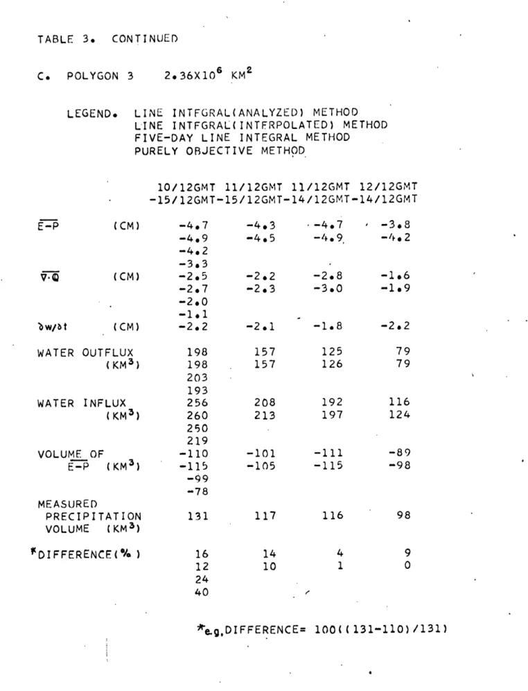
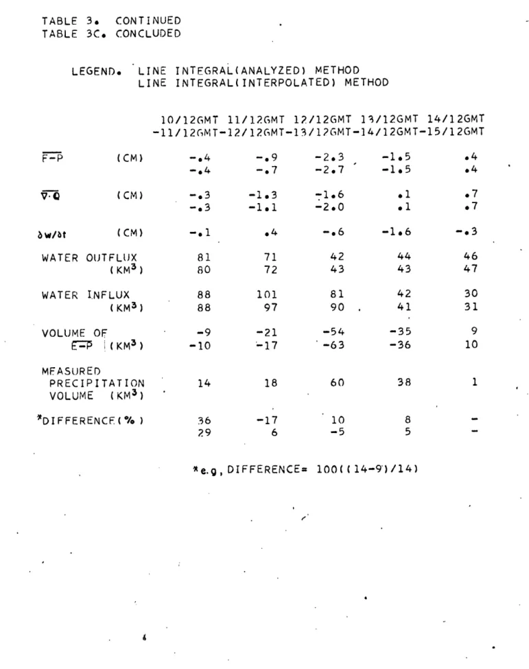
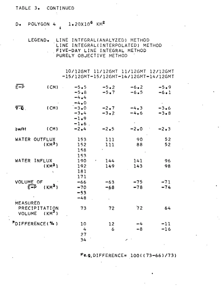
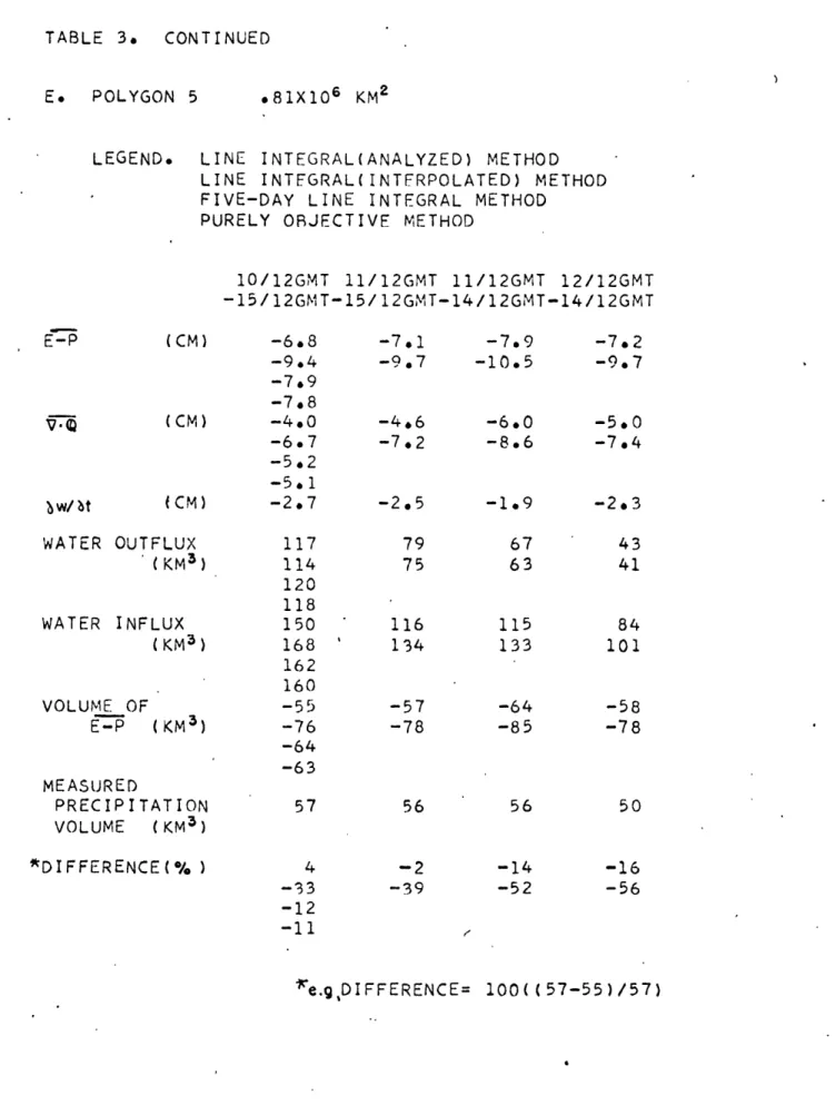
3t Results of line integral methods

42-43 A, Polygon 1 44-45 B. Polygon 2 46-47 Co Polygon 3 48-49 D, Polygon 4 50 51 E. Polygon 5 52-53 F. Polygon 6

54 4, Evapotranspiration volume rates for assumed evapotranspiration of 0. 1 cm day' 1 _{and 0. 5}

LIST OF FIGURES Page F5gure

Number Number

10 1. Subscript notation for a grid network quadrangle

55 2. Areas of consideration using grid point methods 56 3. Polygonal areas of consideration

57 4, The distribution of stations

58 5. Observed 24-hr precipitation ending 12GMT Sept. 116 1961 59 6, Observed 24-hr precipitation ending 12GMT Sept. 12, 19861 60 ., Observed 24-hr precipitation ending 12GMT Sept. 13, 1981

61 8. Observed 24-hr precipitation ending 12GMT Sept. 14 1961

62 9. Observed 24-hr precipitation ending 12GMT Sept. 15, 1961 63 10. Estimated E-P field using Five-Day Integral Method

2. 5ox2. 50 resolution. Time period is 10/12GMT-15 /12 GMT, September 1961.

64 11 Estimated E-P field using Five-Day Integral Methodo

5ozx5 resolution, Time period is 10/12GMT-15/12GMT, September 1961.

65 12. Estimated E-P field using Vertical Profile Method, 2. 5 X2o 50 resolution. Time period is 10/12GMT-15/12 GMT September 1961,

66 13. Estimated E-P field using Vertical Profile Method5, 50o5

resolution. Time period is 101i2GMT-15/12GMT, Sep tember 1961.

67 14, Estimated E- field using Twelve-Hourly Integral

Meth-od, 2. 5°X2. 5 resolution. Time period is 10/ 12GMT-15/12GMT, September 1961.

63 15. Estimated E-P field using Twelve-Hourly Inteural Method,,

5ox5o resolution. Time pev.od is 10t/12GMT-_15/12GMT, September 1961.

Page Number 70 16, Same as fig 15/12GMTo 17. Same as fig. 15/12GMT. 18. Same as fig.

14/12GMT.

11/

12GMT,

28a. field using Twelve-Hourly Integral Method, 2. 50x2, 50 resolution. Time period ia

12/12GMT-13/12GMT, September 1961.

2 9. Same as fig. 14, except time period is 13/12GMT-14/12GMT.

30, Same as fig. 15, except time period is

13/12GMT-14/12GMTo

14, except time period is

11/15, except time period is 11

12GMT-14, except time period is

15, except time period is

11/12GMT-14, except time period is

15, except time period is

12/12GMT-14o except time period is

15, except time period is

10/12GMT-14. except time period is

15, except time period Is

11/12GMT-14, except time period is

15, except time period is

12/12GMT-73 74 76 77 78 79 80 81 Figure Number

Figure Number 31. Same as fig. 15/12GMT. 32. Same as fig. 15112GMT.

14, except time period is

15, except time period is

14/12GMT-Numnber 84 85 86 340 Same as fig. 15/ 12GMT. 35. Same as fig. 14/12GMT, 36, Same as fig. 14/12GMTo

37. Same as fig.

33, except time period is

11/12GMT-33, except tirm period is 11/

12GMT-33, except time period is

12/12GMT-330 except time period is 12/12GMTh

38. Comparison of P (measured),

Estimates of P-E and -~7.Q

P-Er and -t

were made with the Five*Da Integral Method, Time period is 10/12

GMT-15/12GMT, September 1961.

39. Comparison of P (measured). PaE arnd

--Estimates of P-E and -" were made with the Vertical Profile Method, Time period is 10/12GM

aT-15/12GMT, September 1961.

40, Comparison of depth of P (measured), P-E and

-O--Estimates of P-E and --9-:-. were made with the

TwelveHourly Integral Method, a, bo Co d. 64 10/12GMT-11 /12GMT 11 /12GMT-12/ 12GMT 12/12GMT- 13/12GMT 13/ 12GMT-14/12GMT 14/12GMT-15/12GMT

33. Comparison of P (measured), P-, and --~ o

Estimates of P-E and -- ' were made with the Twelve-Hourly Integral Method. Time period is

1i0/l2GMT-15/12GMT, September 1961.

98

88

89

-1vi-Page Figure Number Number

92 41. Comparison of P (measured) and P-E (estimated by L1ine Integral

15712 GMT

Method ), Time period is 10/12

GMT-September, 1961.

41, except time period is 11/12

GMT41, except time period is 11/12 GMT

-41, Except time period is 12/12

41, Except time period is 12/12

GMT-46. Comparison of P (measured) the Purely Objective Method).

15/12 GMT , September 1961.

and P-E (estimated by Time period is 10/12 GMT-92 93 93 94 94 95 48. Comparison of depth of mated by Lne Integal

10/12 11/12 12/12 13/12 14/12 G MT- GMT-GMT= 11/12 12/12 13/12 14112 15/12 P (measured) Method)

and P-E

(esti-GMT

GMT GMT

GMT

GMT

Al. V Q field from Travelers Objective Analysis

Time period is 12/12 GMT- 13/12 GMTo September 1961

47. Comparison of P (measured) and P-E (estimated by the

Five-Day Line Integral Method). Time period is 10/12

GMT - _{15/12 GMT , September 1961.}

96-97

L INTRODUCTION

Physical Basis

This study is based upon the principle of continuity of mass. We

confine consideration to a given volume of atmosphereo bounded at the

sides by permeable walls, at the bottom by the surface of the earth, and

at the top by the outer reaches of the atmosphere, Change in the amount

of atmospheric storage of water substance within the given volume can

occur by three processes: transport of water substance through the wall#,

precipitation, and evapotranspiration, The transport process is the main

concern of this study. The question now naturally arises as to how well

we can measure transport.

The worldwide network of aerological stations supplies wind data and water vapor content data at a number of levels. When vertically

lntegra-ted, these data provide a measure of atmospheric water vapor transport at a given time and geographical location. The most important data in

this study are transport values for the North American network of aero-logical stations, These data are analyzed so that estimates of water substance transports through various walls can be made. Aerological

data contain water vapor content values as opposed to water substance (vapor, liquid, and ice- as in clouds) values. Liquid water content stu-dies by Squires (1958), Warner and Squires (1958) , and Fletcher (1962)

lead us to surmise that the content of water in the liquid and solid phases is small compared to the water vapor content in a corresponding volume

of saturated air, The humidity element of the aerological sounding inutn ment detects a cloud as a region of 100T (or close thereto) relative humi-dity, Therefore, we conclude that the transport of water vapor is a very

close approximation to the transport of water substance. Herein lies our

first assumption.

In order to measure te the transport for any time period, continual observation is, ideally, necessary. Tbis being impractical, it must be

assumed that an observation at a given time is representative of the mean condition for several hours. For example , observations taken every twelve hours must be construed to represent the mean conditions for six hours on either side of observation time, Herein lies our second assump-tion,

History

For over two decades, aerological data over much of the northern hemisphere have been of sufficient quantity and quality to describe the motion of the atmosphere in three dimensions up to the height of the tropo-pause. The use of these data by dedicated investigators has resulted in a better knowledge of the general circulation of the atmosphere.

Investigations of atmospheric water vapor divergence and transport are undertaken for two basic reasons. The effect on the energy budget due to 'he release of latent heat and the transport of latent ener gy has

been a subject for study for over fifteen years. White (1951) was one of the first investigators in this area and investigation ie still in progress as

evidenced by the continual efforts of the Geophysical Fluid Dynamrics Labo-ratory0, Environmental Science Services Administration, Washington D. C.

and individual investigators including Peixoto (1965) and Hastenrath (1966). Another reason for study of atmospheric water vapor is to show its relation to hydrology, Several hemispheric and regional studies have been made. Benton, Blackburn, and Snead (1950) emphasized the importance of the atmospheric branch of the hydrologic cycle. Benton and Estoque (1954),,

in an important study used North American data to show that only a small percentage of transported water falls as precipitation. They also noted that transport is not necessarily proportional to precipitation and that the atmospheric water vapor divergence field can be used to estimate

evapo-transpiration minus precipitation for large areas. Hutchings (1957) in a

regional study of three months duration, used a quadrangular area formed

by the straight lines joining four aerological stations. He assumed that

variation of transport between the stations was linear and computed the net

transport into the area. Values of precipitation and evapotranspiration were

estimated by independent means. Results showed that the net atmospheric transport almost exactly balanced precipitation minus evapotranspiration.

Starr and Peixoto (1958) discussed the water vapor divergence field for the

year 1950 for the entire northern hemisphere. They noted areas of con-vergence over the headwaterw and drainage basins of large rivers and also

over oceanic regions of observed low salinity. On the other hand, diver-gence was noted over oceanic regions of observed high salinity and over

arid regions. An interesting point dwith reference to their study is that it

was begun primarily to investigate the energy budget. However, the

imaplications of the results with respect to to the water budget were so in-teresting th-.t the authors felt compelled to pursue them, Benton (1960) reiterated his previous findindings and additionally discussed the relation be-tween transport, precipitation, and area of consideration. He showed that as the area of watersheds under consideration decreases, the percentage of precipitation resulting from a water source outside of the watershed increases. Rasmusson (1966), in an extremely comprehensive study,

discussed the hydrology of North America, He did not limit the investi-gation to the atmospheric branch of the hydrologic cycle but dealt with the

entire cycle. This caused his verification data to include such items as river streamflow measurements and the time time variation of the levels of

the Great Lakes, His work was accomplished using mean monthly data,

Purpose

In all of the foregoing studies, periods of consideration were at least one month long. Would results for periods less than a month be reasona-ble ? This is one of the questions which we shall attempt to answer.

Ras-muson, using basic periods of one month, howed that the accuracy of water vapor divergence exhibits rapid d eterioration as areas of considera-tion decrease below . 5x106 km 2 (approximately the size of the area bom-n2 ded by 800_{W, 30oN, 95OW, and 47}0_{N). Will periods shorter than a month}

yield deteriorating results for larger areas? 'This is another question which we shall attempt to answer,

Succinctly, the purpose of this study is to investigate the accuracy with which the North American aerological network can depict the atmos-pheric branch of the hydrologic cycle on a short time scale for variously

11, FORMULAE

Let us begin with notation,

= longitude - radians

= latitude - radians

S a time period

a * radius of the earth * 6371. 22 km

g * acceleration of gravity a 980. 6 cm sec° 2

i,

J

io

q * specific humidity - gm kg°1

a = distance along a path - cm t * time - seconds

a zonal (west to east) component of the horizontal wind at a given level - cm see"1

v m= eridional (south to north) component of the horizontal wind at a given level - cm see-1

A * area = cm2

C = a constant

E a evapotranspiration - cm (depth) or km3 (volume)

FN = horizontal zonal water vapor transport at a given level-gm (cm mb

secD-F = horizontal meridional water vapor transport at a given level

P = precipitation - cm (depth) or km3 _(volumeD

Q = horizontal zonal water vapor transport above a point on the earth's surface - gm (cm sec)' 1 or cm2 sec 4

Q+= horizontal meridional water vapor transport above a point on the

earthus surface - gm (cm sec)"1 or cm2 seca1

R * average of adjacent grid point values of Q\ and Q

W = atmospheric storage of water - cm or gm cm' 2

l = unit vector oriented west to east

I

= outward oriented unit normal vector

F

-gm (cm mb sec)"1

(

J

+

ij

m2 sec 1

V=

S* ( ) = horizontal divergence of a parameter ( baSe* the surface value of a parameter

( }usl the value of a parameter at the first even 50 mb level above the surface

( ) = the value of a parameter at the highest even 50 mb level

The following development of equations is due to Starr and Peixoto (1963), At a given level, the horizontal water vapor transport is

At a given point above the earth's surface, the horizontal water vapor

transport is

If we define the time average as

aL( t (3)

then the time average of

ris

and the time average of Q is

We conclude from the discussion of Starro Peixotoo and Crisi (1983), p. 100

that negligible error is introduced by assuming no water vapor transport

above 300 mb. In this study, p.bis usually 300 mb.

We now trace two mathematically equivalent procedurea used to obtain 4~ the same procedures hold for Q o The basic data for both

procedures are the products qu for every level for every synoptic time. In the first procedure, qu for each level is obtained by the relation

These values of qu at each level are vertically integrated by the relation

which is similar to ( 5 ), Due to the arrangement of raw data, it was convenient to find r N for 00 GMT and 12 GMT separately. In cases

when some values of qu were missing in ( 6 ), a correspondingly snall-er n was used, The shortcomings of this procedure are discussed in the nent

section The second procedure finds the vertically integrated tranport for

each synoptic time by the relation

%tA (8)

which is similar to (2)o QX is found for any n- day period (assuming

observations every twelve hours) by application of the trapezoidal rule

4

Z*

-.

k

=

(j4)oo

t

\0QAT

Atmospheric storage is defined by P.s,

CO

(10)

Since data0 in this study, are available for every 50 mb, the integral in ( 10 ) is evaluated by the trapezoidal rule as follows:

V\LqAx

--

t

S O)

1

+

+

o)Nj

By defL ng

and

we may rewrite (11) in the form

The units of W in thi form can be shown to be cm or gm cm' 2 °Simi-lar relations are formulated for Qx and Q with w the resultant units o

gnm om sec) 1 or cm2 ec "

Using analyzed fields of zonal and meridional water vapor transport,

the divergence field of the water vapor transport ( to) is calculated, If

we consider a vertical column of air with unit cross section, the net gain of water, E-P , must be balanced by the divergence and the change in

atmospheric storage, That is,

In geographical coordinates, '7 is expressed in the form

In finite difference form, for each 2. 60 x 2. 50 quadrangle in the grid net=

work of figure 2, the equation takes the form

where

Q

7.

tr

Z

I(d.X-',c-

I

Subscripts are self-explanatory upon reference to the

figu

j41t

j-t j+I

Figure 1. Subscript notation for a grid network quadrangle.

ire belowo

tl

;81,jc+

\

+(Q

r)k~

,-d

Equation (15) i< further reduced to

where C varies proportionately with the period of time under considera-tion as shown in table 1i

Table 1. Time dependent constants for finite difference divergence equation. 2. 5S x 2. 50 grid network or 30 days 5 days 4 days 3 days 2 days I day 12 hours

C .09340 .01555 .01244 .00934 .00622 .00311 .00156

Values of atmospheric storage ( W- sometimes called precipitable water )

for each quadrangle are estimated by averaging the four W values at the vertices of the quadrangle. Change in atmospheric storage ( -4 ) is

computed by subtracting the value at the beginning from the value at the end of the time period. The resultant value of - + I is in units of cm, To obtain a volume estimate, this value is multiplied by the area of the quadrangle. The sum of appropriate quadrangle E-P estimates com-prises the volume estimates of E-P for the areas of figure 2. Likewise,, the sum of all the E-P quadrangle volumes which are negative comprises an estimate of the actual precipitation volume.

Another method of calculating (o for a given area is to use

Gauss' Divergence Theorem in the form

nicely to the use of transport values at aerological stations lying on 9. In this case. ( 17 ) becomes

where n is the total number of stations, each of which is consecutively

numbered about the enclosed path. & S is the distance between

station I and station i+1. Estimates of 'Q(t were made with equation

( 18 ) for the six polygonal areas shown in figure 3. It will be noted that in the use of ( 18 ), we make the implicit assumption of linear transport variation between stationst This was the procedure emiployed by

HI., THE CONSEQUENCES OF MISSING DATA

In the preceding section, it was noted that station values of Q>

and Q # derived by first computing qu and qv lead to some difficulty when some of the basic data is missing. We shall briefly discuss this problem review the approach of other investigators, and suggest methods for minimizing it.

If values of qu (this discussion applies to qv also) are missing, it is obvious from (6) that qu becomes less accurate as n decreases, In studies which cover long periods of time, it is expected that missing

values will be random with a resultant negligible effect on the accuracy of

qu. It should be noted that one of the strengths of general circulation observational studies is that the long periods of investigation tend to aver-age out the random error of individual observations. This was the

assump-tion in the one year study of Starr and Peixoto (1958), and the six month study of Starr and Peixoto (1963). This rmethod lends itself nicely to computer operation using raw data ( q, u and v ) input and has recently proved successful for periods as short as one month as shown by Rasmusson

(1966).

Benton and Estoque (1954) who worked with basic periods of one month, substituted interpolated values for all missing data. Hutchings

(1957), in a three month study, estimated values of missing data by

In this study of short time period's, the assumption of random missing reports is likely to be a poor one, especially if the short time period has rapidly changing features. As an example, consider the

daily 500 mb zonal winds at Shreveport, La, for 00 GMT 11-15 September 1961. Data for the 1 th and 12th were missing but, from analyses, could be estimated as -12 meters sec 1 and -10 meters

sec" , respectively, 13th, 14th and 15th data were 7 meters sec lo 9 meters sec"1 and 9 meters secl , respectively. A comparison of the zonal wind average with and without the estimated values for missing data yields 0. 6 meters sec*1 and 8. 3 meters sec l , respectively, Per-forming an accurate analysis with an erroneous qu at one station would demand heavy reliance on neighboring stations. If, however, the neighboring stations also have qu values derived from less than a

complete data set, with missing reports from days which aren't the same

as our original station, then the analysis becomes very subjective indeed. In dealing with this problem several alternatives seem to present themselves. The first is to analyze, as best as possible, for the Q and Qi values which we know aren't completely correct, These anal-yses will be very difficult. The second is to analyze qu and qv at

each of the levels. This will be a bit less difficult but will require great subjectivity. Both of these are attempted, as Is noted in section IV.

Another alternative,, designed to minimize the problem, is to par-form analyses of Qh and Q $ fields for each synoptic time within the

pEriod of conideration. These ana1yzed fields supply wlues, for those stations 3with missing data, which can be used in equation (9). Alterna-tively, the analyzed fields can be read for a grid network before applying equation (9). It has been noted by Rasmusson (1966), pp. 39-40, that this latter method tends to remove part of the random analysis error, thereby resulting in a smoother divergence field.

Still another alternative is to analyze the basic q, u, and v fields for every synoptic time for every level resulting in values of these

parameters on a grid network. A field is then computed for any desired time period. Although this seems like a straightforward method of getting the job done, the amount of work involved is staggering, If,

as in this study, sixteen levels are used, a total of 48 analyses are

necessary for each synoptic time. This herculean task is well adapted

to automatic objective analysis methoda, Therefore, the objective

anal-ysis technique developed by personnel of the Travelers Research Center was utilized for a one day period. This procedure is discussed in the appendix.

IV. DATA AND PROCEDURES

Values of q, U, and v, at the surface and at every 50 mb interval up to 300 nib, for 00 GMT and 12 GMT were used for the aerological stations shown on figure 4. In cases when the radiosonde humidity

ele-ment is "motorboating" due to very low humidity or low temperature, a

statistical value is used. The statistical values are a set of mean values of relative humidity for use, at various temperatures, when the humidity element is below its operating range.

Northern hemisphere data of this type for a five year period

beginning in May 1958 were originally collected jointly by the U. S.

Weather Bureau and the U. S. Air Force. Further processing of the data was performed jointly by the Travelers Research Center and MIT's Planetary Circulations Project. The result of this massive collection and processing effort is a collection of 120 magnetic tapes containing data from 704 northern hemisphere stations for 60 months. This collection is part of the MIT General Circulation Library. The magnetic tapes for September 1961 were used in the present study,

One very important decision at the very outset was the type of weather situation with which to deal. It was thought necessary that the situation fit two basic requirements. Its major features should be within the confines of available data, and some means of verifying results should be available, The first requirement was difficult to fulfill due to the

* ~1

normal progression of weather systrnms. Therefore, the second require-ment became the more important determining factor

Due to the efforts of LaRue and Younkin (1963), there are available large scale precipitation volumes and distributions for the most

signifi-cant storms over the United States (east of 1050W) and Canada (south of 490N) during 1961, LaRue and Younkin present tables of isohyetal areas

and volume estimates for the two greatest 24-hr storms in each month and the four greatest 48, 72 968 and 120-hr storms of the year. These precipitation volumes will be our principal means of verifying the volume

estimates made from aerological data, These measured precipitation volume values were derived by analysis of the 24-hr observed precipitation

charts prepared daily at the National Meteorological Center, One storm

produced the largest volume for all of the duration categories. The

per-iod of this storm--12 GMT 10 September 1961 to 12 GMT 15 September 1961--was chosen for consideration. In such a storm, precipitation vol-umes greatly exceed evapotranspiration Therefore, we assume that evapotranspiration is negligible. Even in a storm of such wide areal extent, there will be periods of little or zero precipitation for some of our areas of consideration (figures 2 and 3). In these cases, the esti-mated E- will likely be positive rendering our precipitation volumes unusable for verification. The estimated E-P, in such a case, should

be a reasonable estimate for evapotranspiration,

12 GMT 11-15 September 1961 are shown in figures 5-9. VoluIe

estimates for the areas and polygons of figures 2 and 3 were made by: I1) estimating the area of each isohyet interval which fell within the individual areas and polygons,

(2) estimating each isohyet interval volume in the same area-volume proportion as presented by LaRue and Younkin, and

(3) adding the results.

The volume estimates are listed with other results in tables 2 and 3. As indicated, the period from 12 GMT 10 September 1961 to 12 GMT 15 September 1961 is the prime period of consideration,

Accordingly, several different methods of estimating E-P for this five day period are attempted. Since this is somewhat of a pilot study several different procedures are appropriate. Various methods of attack are useful since they show if the data can stand the test of manipulation and still give fairly consistent results.

Grid Point Methods

The first of these -- the Five-Day Integral Method - begins with the computation, for each station of- figure 4, of the vertical integralso, Q X and Q o separately for 00 GMT 11-15 September 1961 and 12 GMT 11-15 September 1961o Analyses of these fields are attempted even though much subjectivity is necessary (see section III). After analysio, values of Qx and Q are read--for a 2, 5 latitude by 2, 5o longitude

grid network delimited by the boundary of area 1 on figure 2-oand used to compute the divergence ( -- ) field for the five day period. The

resultant divergence field is added to the change in atmospheric storage ( \dJt ), described by the W fields at the beginning and the end of the period, resulting (by equation 13) in an estimate of E-P for each

2. 5o x 2. S0 quadrangle, A coarser resolution is accomplished by aver-aging the four 2.50 x 2. 50 estimates within each even So x 50 quadrangle. The same divergence result would have been attained by using a 50 x 50 grid network. It is expected that the change in atmospheric storage, although not exactly the same, should be very nearly the same,

A second method-the Vertical Profile Method-ois essentially the same as the Five-Day Integral Method except that each level is con-sidered. It begins with analyses of qu atd. qv for 00 GMT 11-15 September 1961 and 12 GMT 11-15 September 1961 for the surface and each 50 mb level up to 300 mb, Values of qu and qv are read for the grid network at every level and the vertical integrals, QN and Q4,

are computed for each grid point. The procedure, after computation of the vertical Integrals, is exactly the same as above. Although this method is also subjective, the computation of the vertical integral from the analyzed levels should tend to reduce the random analysis error and the grid point reading error, This method offers the opportunity to investigate the vertical structure of the transporta From these sixteen (one for each level) grid matrices, we obtain a rather detailed vertical

distribution for every 2.o 5 of latitude and 2, 5o of longitude. Our original purpose in dealing with the vertical structure of the transport was to study the vertical convergence of water into a storm. However, since the storm was not completely contained within the confines of our data, the cross sections which were constructed are not shown, They bear great similarity to those already presented by Benton and Estoque

(1954) and by Rasmusson (1966).

If we consider twelve-hourly observations to be representative of a time period spanning twelve hours, the period covered by the above methods is actually 18 GMT 10 September 1961 to 18 GMT 15 September 1981.

A third method--the Twelve-Hourly Integral Method--begins ~i th analyses of the vertical integral fields, Q and Q+ for the eleven

12-hourly synoptic times from 12 GMT 10 September 1981 to 12 GT 15 September 19681. Values of Q- and Q+ are read for the grid network for each time and are used in the trapezoidal rule relation (equation 9) to find values of Qx and for an n-day period. These Q and Q flelds, along with the appropriate W fields, are used to compute E-P for any desired time interval from twelve hours to five days (or longer if additional consecutive analyses are available). The time intervals considered are: each 24-hr period ending at 12 GMT for the five days

11-15 September 1961, 12 GMT 10 September 1961 to 12 GMT 15 September 1961, 12 GMT 11 September 1961 to 12 OMT 15 September 1961, 12 GCIMT

11 eptemnber 1961 to 12 GMT 14 PS1perber and u96 i 12 GMT 12 Sept-emnber 1961 to 12 GMT 14 September 1961., No previous knowledge of the precipitation pattern is necessary in usin this method,

The methods described above have been used to estimate E-P for

the areas, ranging from . 24 x 106 km2 _{to 6., 67 x 106 km2, shown in}

figure 2,

Line Integral Methods

A fourth method, which further reduces subjectivity, is the use of

a line integral around a closed polygon with aerological stations at its vertices. By Gauss' Divergence Theorem (equation 17), we know that the net outflux through the boundaries of such a polygon can be euated to

divergence, Several polygons, ranging in size from .32 x 106 km2 to 56 83 x 106 km2 , _{were selected for investigation (see figure 3). In using}

this method, a station's consecutive twelve hourly vertical integrals are combined by equation (9) to give results for any desired time period,

The time periods considered with this method are the same as listed under the Twelve-Hourly Integral Method. In the case of a missing vertical integral, two procedures are used to estimate the misslng value. The first procedure is to read X and ~ values for the station from the TweIve-Houryl Integral Method analyses. Th,e second procedure is a linear temporal Interpolation providing that only one consecutive integral is .nsising ff more than one consecutive integral is missing, sufficient

estimates are made by the first procedure so that no more than one consecutive integral has a missing value and then linear temporal

inter-polatlon is performed, No intentional bias is introduced when selecting

which of an even number of consecutive missing integrals are to be read from analyses, We now assign the two titles--Line Integral (Analyzed)

Method and Line Integral (Interpolated) Method--to the foregoing

pro-cedures. To account for the change in atmospheric storage, those values of W for grid points which are within or on the boundary of each

polygon are considered. The specific procedure is to average all such W values at the end of the time period and subtract the average at the beginning of the time period.

Further methods are merely slight modifications of those already described but for the sake of clarity they are given descriptive names.

The Prly otjective Method takes a weighted average, for each

station, of the computed values of QN and Q4 for 00 GMT 11-15

September 1961 and 12 GMT 11-15 September 1961 which were used in the Five-Day Integral Method. The weighting is based on the number of

levels, below 750 nb, which are included in the 00 GMT and 12 GMT values. These averages are then used in a line integral to determine divergence for the various polygons by Gauss' Theorem. The change in atmospheric storage is added as in the previous line integral methods. This method is entirely objective except for the inclusion of atmospheric storage considerations. No attempt is made to estimate missing reports.

It is expected that results from this method will compare unfavorably with the other results,

The Five-Day IAne Integral Method makes use of the analyses

accomplished in the Five-Day Integral Method, Analyzed values are read for each station whose QN and Q. were computed from less than a complete set of input data; otheritee, computed values are used.

These values are used in precisely the same manner as in the previous

paragraph.

The water influx and outflux are presented since they are of

interest and are calculated in the course of the computation of divergence in the line integral methods.

V. RESULTS AND DISCUSSION

A complete set of results is presented in tables 2 and 3, and

figures 10-48. The results of the objective analysis by Travelers Research Center are presented in the appendix.

The results are quite voluminous; therefore, no detailed

dis-cussion is presented. Tables 2 and 3 are self-explanatory, with the

possible exception of the meaning of "Difference". This is the

per-centage error incurred when using t +eQ (which is referred to as E-P or estimated E-P in all of the results) as an estimate

of the measured precipitation. "Difference" is not calculated when measured precipitation is very small or zero. Figures 33-48 are pictorial representations of some of the results listed in tables 2 and 3.

Areal Distribution by Grid Point Methods.

The selection of a basic 2. 50 a 2, 50 grid network does not iram

ply that accurate results can be obtained for each quadrangle. It was

chosen as a convenient framework on which to work, and should usually result in moderately successful areal distributions. It is interesting to note that grid point reading errors of 50 gm (cm sec)l--in many cases, accuracy was not as close--could cause a maximum error of 0, 4 km 3 day"1 or approximately 0. 7 cm day"1 for a 2o. S x 2a 50 quadrangle.

When making comparisons between the observed precipitation charts and the estimated E-P fields, it should be noted that the units

are inches and centimeters, respectively.

The areal distribution of estimated E-P for the various periods of consideration are shown in figures 10-27 and 29-32. The divergence ( 0Q ) field of figure 28 is included for comparison with the Travel-ers Research Center objective analysis shown in figure Al.

This brief discussion is limited to the E-P fields for the entire five day period. Figures 10 and 11 show marked similarity to figures

12 and 13. This is to be expected since all were derived from subjective analyses performed by the same analyst. Both distributions have accen-tuated the large rainfall in southeast Texas and along the path of the storm, but they have not indicated some areas of lesser rainfall. As an example, there is no indication of negative E-P in eastern North Carol-ina, yet precipitation of over one inch occurred there.

Figures 14 and 15 show patterns somewhat similar to the previous figures. There Is some major difficulty which caused an area of diver-gence to appear over Texas, Louisiana, and Oklahoma. This difficulty can be traced principally to the 00 OMT 12 and 13 September 1961 synop-tic times. Stations 240, Lake Charles, 248, Shreveport and 340, Little Rock, were missing on 12 September 1961 and stations 240, Lake Charles, 259, Fort Worth, and 353, Oklahoma City, were missing on 13 September

1961. An attempt was made to keep continuity between analyses when data were missing, but the nature of the problem at hand--estimating the small difference of two large values--demands complete data coverage.

-A serious problem with the diatributions is the ccrrence o* large positive values of E-P o This indicates a very large evapo-transpirationd That these values are overestimates is verified by reference to U. S. Weather Bureau climatological data surveys for September 1961. These surveys contain values of measured "pan" evaporation which are generally acknowledged to be overestimates of

actual evapotranspiration. The five day average of the recordings of

"pan" evaporation for Tennessee, which is within the area of our lar-gest positive E-P, is 4. 6 cm. The comparison of this figure-an overestimate- -with the estimated E-P values on the above figures

clearly illustrates the magnitude of this problem.

The remainder of the grosp of figures from 16 to 32 show

straength and weaknesses similar to those noted above.

We can conclude, in a very broad sense, that these distributions generally describe the precipitation pattern but the omission of key stations with respect to the precipitation can render the resultant dis-tributions inaccurate. Ra mnusson (1966) emphasized the importance

of smooth analyses to avoid the formation of divergence "couples" (the

repeated altering of sign between adjacent rows or columns in the grid network). It is difficult to derive a smooth analysis for a short time period. However, to obtain meaningful divergence patterns, a certain

amount of judicious smoothing must be accomplished.

scale is

the fact Chat

dif-ferent ord.er. That isa during a ranal, evapotrranspiration is

negli-gible compared to precipitation, Consider two adjacent areas, A and

B. of the same

size. It is raining in A but isn't raining in B. During

the rainfall, the precipitation in A is likely to be much greater than

the evapotranspiration in A, which, in turn, is greater than the

evapo-transpiration in Be If we have data from one, two or more aerological

stations in and around the areas, will it be possible to show

conver-gence over

A

and divergence over B? If this is possible, and let's

assume for the moment that it is, will the data be capable of describing

the tighter gradients over A compared to the loose gradients over B?

An appreciation of these problems gives some insight into the reasons

for having obtained some large positive E-P values. Since the

anal-yzed fields are transports, and divergence is a derived field, it is

almost impossible for the analyst to be aware of moving from an area

of convergence to an area of divergence, Hence, the gradients remain

approadmately the same.

The implications of marginally successful water vapor

diver-gence patterns reach beyond a consideration of the water budget. The

field of vorticity, a parameter derived from the wind distribution, must

suffer from the same type of errors which cause less than completely

accurate water vapor divergence results.

4>8-Volume estiattes by gridl point mehtds,

It was originally expected that larger areas would yield the best results. A glance at figures 33-40 seems to give opposite results

but these cannot be accepted entirely at face value. It will be recalled

that the method of obtaining these E-P volume estimates was to multiply the area by the computed depth and then sum these products for the quadrangles which fell within each area of consideration. Thus,

we are nullifying the effect of some of the negative quadrangles by adding positive quadrangles. It would therefore be expected that the resultant P-E (notice change of sign) volume estimates would gener-ally be less than the measured precipitation. Table 4 gives daily

evapo-transpiration volume rates, for the areas of consideration. resulting

from 0. 1 cm and 0. 5 cm of evapotranspiration. The latter figure is a strong evapotranspiration. A rate, somewhere in between the values

shown, when multiplied by the uiLtable number of days and added to

P-E , should result in a value close to the measured precipitation. Along these lines, it may be argued that the P-E volume, if

used as an estimate of actual precipitation should be comprised of only those quadrangles which showed excess of P over E, It can further be

stated that this volume would be merely a lower botuad on the Irecipita-tion since it also contains some evapotranspiraIrecipita-tion, These argumens, are perfectly valid and must be considered, They have not been treated

hera but would constitute an excellent extension of

studyo Th

problems likely to be faced are similar to those mentioned in the dis-cussion of the areal distribution of -- P. One of the variables which would need careful study is the grid distance, since it is obvious from

the comparisons of the 2, Sox 2o 5o resolutions and o50 x 50 reaolutions (figures 10-32) that grid distance is an Important factor.

Volume estimates by line integral methods.

These results are very similar to those obtained above, It should be noted that since the areas of consideration are different than the areas used in the grid point methods, a detailed direct comparison

cannot be made.

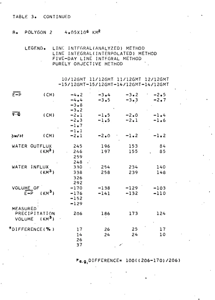
A comparison of the interpolated method and analyzed method

can be made by inspecting figures 41-45 and 48, The results of the

analyzed method are almost consistently lower, This indicates that the effect of analysis, even when playing such a small role as in this method, is to smooth, However, a danger in depending completely on inter-polation is illustrated when considering polygon 5. In this case,

tem-poral interpolation caused a spurious influx as shown in figures 41-44.

General

The following points are worthy of note.

A. Consideration of is necessary for short time periods. B, Since the results of the line integral methods compare favorably

with the grid point methods, certain conclusions can be drawn,

(1) The data can stand the test of manrpulation.

(2) The analyses performed in the present study did not show a great deal of nonlinearity between stations. Therefore, given the choice of finer data resolution In space or finer data resolu-tion in time, this investigator would choose the latter.

C, One complicating factor for studies of this type in the south central

region of the United States is the nocturnal low level jet which occurs at levels of maximum moisture, The occurrence of such a

phenomenon is a strong point in favor of more frequent observations.

This factor has been discussed by Rasmusson (1966).

D, One of the precautions at the outset was to consider areqs to the

east of the Rocky Mountains. Therefore, the accuracy of results achieved would probably be different If mountainous terrain were considered.

The following "Difference" values are from theAne Inte grl

(AnalyMed) Method and the Twelve-Hourly Integral Method results. For

pedods longer than one day, percentage error ("Difference") for area

larger than 1.5 x 106 km2 ranges from +4% to +38%. The range for areas smaller than 1.5 x 106 km2 is -16% to +37%, The consideration of evapotranspiration as discussed under "Volume estimates by grid point methods" would, in most cases, Improve these results. When

considering these results, it should be recalled that only one case for each time category (2-day, 3-day, 4-day, and 5-day) was considered,

For one-day periods, five separate cases were studied. For

areas larger (smaller) than 1.5 x 106 km2, percentage error ranged

from -62% (-70%) to +260% (+70%). There were also some percentage errors not calculated due to very low precipitation, The volume

esti-mates for these one-day periods were within a factor of three except

for:

(1) cases with very little precipitatiorn and

(2) the 34-hr period ending 12 GMT 15 September 1961 for area 1(table 2A). In this case, precipitation ended early in the period resulting in significant evapotranspiration,

When beginning this study, one of the objectives was to determine the minimum length of time and minimum area for which the distribution

of North American aerological stations could accurately depict the

atmospheric branch of the hydrologic cycle° The results of this study, strictly speaking, apply only to the specific periods considered, but they can be used as a base of comparison when w similar studies are attempted, It would appear that the minimum length of time for which reasonable results are obtained is two days, The corresponding minimum areal extent cannot be defined since results appeared reasonable down to the

smallest area considered. These conclusions must be accepted with caution since they were derived from one particular type of synoptic

situation, and from one set of twelve areas of consideration. Also, among the nine periods of consideration, there was only one two-day period. Additional cases, using the methods developed in this study,

must be investigated before firm conclusions can be made, These cases should be investigated with two different methods of attack, The

first method should use the line integral, thereby forming a basis for

the investigation of areas which have no data sources within them. The second should use objective analyses of the vertically integrated fields of water vapor transport. These analyses should be performed for

every synoptic time in the period of consideration, and should be capable of analysis in the three dimensions of longitudeo latitude, and time (the fourth dimension is implicitly included in the vertical integrals). Objeco tive analysis is a necessary prerequisite to the use of these methods on

an operational basis. The strongest point in favor of the success of such endeavors is the firm physical basis upon which they rest. To conclude,

we observe that the methods employed have shown encouraging results. Further research should prove even more promising,

My residence at MIT has bee made po-sible by the U. S, Air

Force through the Advanced Weather Officer training program of the Air Force Institute of Technology. The program has been enriching, and I am extremely grateful to have been afforded this opportunity.

I am thankful for the guidance, timely suggestions, and keen

insight provided by Prof. Victor RP Starr. Prof. Jose P. Peixoto has offered astute advice. The impetus for this study came from an

enthu-siastic researcher whom I am happy to have as a colleague and friend,

Dr. Eugene M. Raamusson. His continual interest was a constant source of encouragement.

Mr, Salomon F. Serouasi of Mitre Corp.0 Mr. Howard M. Frazier of Travelers Research Center, and Miss Judy Roxborough of MIT handled

the large data processing requirement. Special assistance was provided

by the U, S, Air Force 433L prograa. Computation was accomplished

at the MitrheCorp. and the MIT Computation Center.

Credit for figures 5-9 is due to Mr. R. J. Younkin of the National M4teorological Center- ESSAo Sergeant A. Moreau of the Environmental Tlchnical Aplications Center, U. S. Air Force, also provided precip i taiion in for mationo

I am e.remrely grateful to Miss Isabelle Kole for her ambitious wcrk throughcut several weeks in drafting the figure. Miss iRuth B

BIBLIOGRAPHY

Benton. G. S., 1960: Quantitative relationships between atmospheric vapor flux and precipitation. Int. Assn. Sci Hydrology, Pub. No, 51, pp. 60-70,

Benton, Go. S., Blackburn, R. T., and V. O. Snead, 1950: The role of the atmosphere in the hydrologic cycle. Transactions,

American Geophysical Union, 31, pp. 61-73.

Benton, G. So and M. A. Estoque, 1954: Water-Vapor Transfer over the North American Continent. J. Meteor,, 11, pp. 462-477. Fletcher. N. H., 1962: The Physics of Rainclouds, pp. 8-15. Cam=

bridge University Press, Cambridge, England. 386 pp.

Hastenrath. S. L., 1966: On general circulation and energy budget in the area of the Central American Seas., J. Atmos. Sci. 23, 694-711.

Hutchings, J. W., 1957: Water Vapour Flux and flux divergence over Southern England: Summer 1954. Quart. J. R, Met, Soc., 83. pp. 30-48.

LaRue J A,, and R. J. Younkin, 1963: Large-Scale Precipitation Volumes, Gradients, and Distribution. Mon. Wea. Rev., 91,,

pp, 393-401.

Mather, J. R., 1961: The climatic water balance. Publications in Climatology, XIV, No. 3, pp. 251-264. C. W. Thornwaite Associates, Laboratory of Climatology, Centerton, N, J. Peixoto J. P., 1960: On the global water vapour balance and the

hydrological cycle, Tropical Meteorology in Africa, Munitalp Foundation, Nairobi, 1960,

also, Studies of the Atmospheric General Circulation. IV. Planetary Circulations Project, Department of Meteorology, MITo pp. 198-209,

Peixoto, J. P., 1985: On the role of water vapor in the energetics of the general circulation of the atmosphere. Portgal. Phys,o 40

pp. 135-170.

also, Studies of the Atmospheric General Circulation. V. Planetary Circulations Project, Department of Meteorology, BMIT, pp. 138-168.

Rasmusson, E. M., 1968: Atmospheric Water Vapor Transport and the Hydrology of North America. Report No. Al., Planetary Circu-lations Project, Department of Meteorology, MIT, 170 pp.

Squires, P., 1958: The spatial variation of liquid water and droplet con-centration in cumuli. Tellus, 10. pp. 372-380.

Starr, V. P. and J. P PPeixoto, 1958: On the global balance vapor and the hydrology of deserts. Tellus, 10, pp.

of water

Studies of the Atmospheric General Circulation, IV , Planetary Circulations Project, Department of Meteorology. MIT,

pp. 162-197.

Starr, V. P., Peixoto, J. P., and A. R, Crisi, 1963: Hemispheric water

balance for the IGY. Scientific Report No, 4 . Planetary

Circula-tions Project, Department of Meteorology, MIT, 32 pp.

Tiadale, C. F., 1961: The weather and circulation of September, 1961. Mon. Wea. Rev. . 89. pp. 560-566.

U. S. Department of Commerce- Weather Bureau: Climatological

Data-State Monthly Summaries . September, 1961.

Warner, J. and P. Squires, 1958: Liquid water content and the adiabatic model of cumulus development. Tellus , 10, pp. 390-394.

White, R. M., 1951: The meridional eddy flux of energy. Quart. J, R. Met. Soc., 77, pp. 188-199.

-36-TAB L 2. RESULTS OF GRID POINT '!JTTHODS SEE ALSO FIGUREF 2 AND 33-40.

A. AREA 1 6.67X10'6 KM1

TW:-LVE-HOURLY ITTFGRAL METHOD

1O/12GMT 11/12GMT 1.1/12GMT 12/12GMT -15/12GMT-15/12GMT-14/12GMT-14/12G'. U -p (CM) 9.Q (CM) VOLJM F E- (KM5 ) M-E ASURED PRECIPITATION VOLUME ( KM'I ) DIFFFRENCE(0/) -2.6 -1.2 -1.4 -176 253 30 -2.1 -. 8 -1.3 -143 222 36 -2.1 -1.2 -1.0 -142 193 26 S -1.5 -,6 -. 9 -103 142 27 10/12GMT 11/12GMT 12/12GMT -11/12GMT-12/12GMT-1/12GMT 1/12GMT 14/12GMT -14/12GMT-15/1 2GMT -(CM) V Q, (CM) VOLPIF OF F-P . (KM3) MEAS [RE D PReCIPITATION VOLIUME ( KM 3) DIFFERENCE( /.) FIVE-DAY INT EGRAL MET HO ) 10/12GMT VFRTI CL PROFILE '"ETHOD S0/ 12lGMT -15/12GMT- 5/12GMT (CM) (CM) ( CM) VOLU~" 'OF 5-P (KM) M- A ,S l P C r.

PRFCI P ITA TIOON

VOI UF E (K') DI FFFRENCE (°Io) -2.7 -1.2 -1.4 -179 253 29 -3.5 -2.1 -1.4 -236 253 7 100((253-176)/253) -. 5 -. 4 -. 1 -32 31 -3 -. 6 -. 1 -38 52 27 -. 9 -. 2 -. 6 -61 -. f .4 -. 4 -. 6 -. 4 -. 2 -42 77 45 -_r

vWIN

TABLE 2. CONTINUED

Be AREA 2 4,29X106 KM2

TWELVE-HOURLY INTEGRAL METHOD

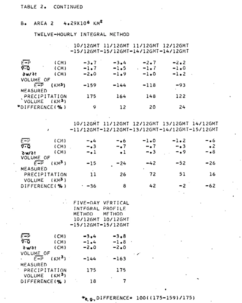
10/12GMT 11/12GMT 11/12GMT 12/12GMT -15/12GMT-15/12GMT-14/12GMT-14/12GMT E-P (CM) * (CM) aw/bt (CM) VOLUME OF -P (KM3) MEASURED PRECIPITATION VOLUME (KM3) *DIFFERENCE(o% ) -3.7 -1.7 -2.0 -159 175 9 -3.4 -1.5 -1.9 -144 164 12 -2.7 -1.7 -1.0 -118 148 20 -2.2 -1.0 -1.2 -93 122 24 E-P (CM) vIQ (CM) aw/bt (CM) VOLUME OF E-P (KM3 ) MEASURED PRECIPITATION VOLUME (KM3 ) DIFFERENCE( % ) 10/12GAT -11/12GMT--. 4 -. 3 -. 1 -15 11 S-36 11/12GMT 12/12GMT -. 6 -. 7 .1 -24 26 8 12/12GMT -13/12GMT -1.0 -. 7 -. 3 -42 72 42 13/12GMT -14/12GMT -1.2 -3 -. 9 -52 -2 14/12GMT -15/12GMT -. 6 *2 -08 -26 -62 FIVE-DAY INTFGRAL METHOD 10/12GMT E-P (CM) V.O (CM) Saw/t (CM) VOLUME OF E-P (KM3) MEASURED PRECIPITATION VOLUME (KM3) DIFFERENCE(% ) VFRTICAL PROFILE MFTHOD 10/12GMT -15/12GMT-15/12GMT -3.4 -1.4 -2.0 -144 175 18 -3.8 -1.8 -2.0 -163 175 7 100((175-159)/175) *e.gQ.,DIFFERENCE=

TABLE 2. CONTINUED

C. AREA 3 3.27X10 6 KM2

TWELVE-HOURLY INTEGRAL METHOD

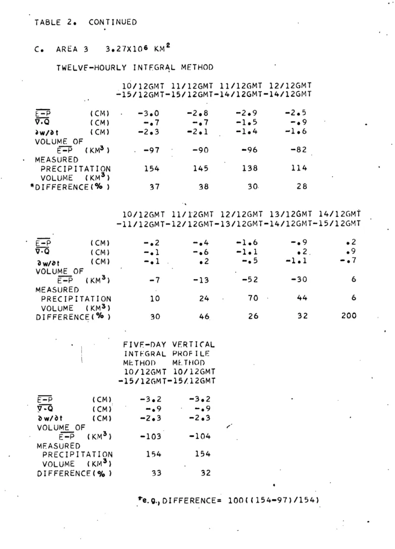
10/12GMT 11/12GMT 11/12GMT 12/12GMT -15/12GMT-15/12GMT-14/12GMT-14/12GMT E-P (CM) V.Q (CM) Sw/at (CM) VOLUME OF E-P (KM3 ) MEASURED PRECIPITATION VOLUME (KM3 ) *DIFFERENCE(% ) -3.0 -. 7 -2.3 -97 154 37 -2.8 -. 7 -2.1 -90 145 38 -2.9 -1.5 -1.4 -96 138 30. -2.5 -e9 -82 114 28 10/12GMT 11/12GMT -11/12GMT-12/12GMT 12/12GMT 13/12GMT -13/12GMT-14/12GMT-14/12GMT 15/12GMT E-P (CM) V.Q (CM) a w/at ((CM) VOLUME OF E-P (KM3) MEASURED PRECIPITATION VOLUME (KM3) DIFFERENCE(% ) FIVE-DAY INTEGRAL METHOID 10/12GMT VERTICAL PROF I LE ME THOD 10/12GMT -15/12GMT-15/12GMT E-P (CM) Y-Q (CM) bw/ t (CM) VOLUME OF E-P (KM3) MEASURED PRECIPITATION VOLUME (KM3 ) DIFFERENCE(% ) -3.2 -9 -2.3 -103 154 33 -3.2 -9 -2.3 -104 154 32 100((154-97)/154) -. 2 -. 1 -. 1 -7 10 30 -. 4 -. 6 o2 -13 24 46 -1.6 -. 5 -52 70 26 -. 9 .2. -30 44 32 .2 .9 -7 6 6 200 *e. g. DIFFERENCE=

TABLE 2. CONTINUED

D. AREA 4 1.82X10 6 KM2

TWELVE-HOURLY INTEGRAL METHOD

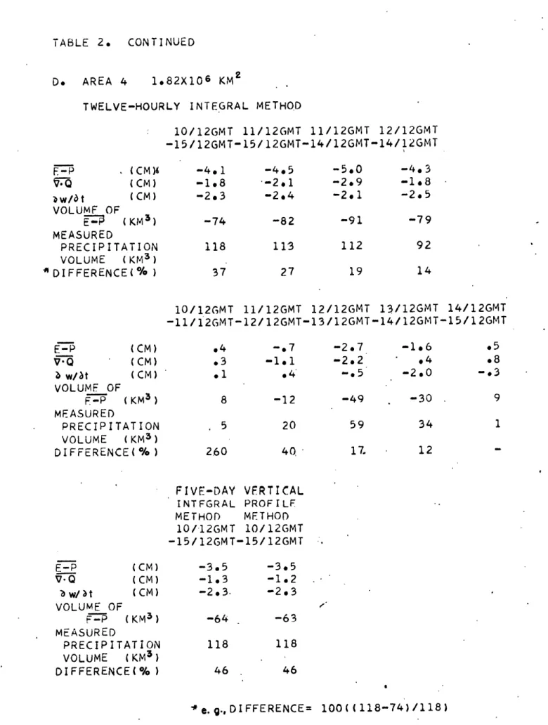
10/12GMT 11/12GMT 11/12GMT 12/12GMT -15/12GMT-15/12GMT-14/12GMT-14/12GMT F-P (CM)A -4.1 -4.5 -5.0 -4.3 q Q (CM) -1.8 --2.1 -29 -1.8 zw/bt (CM) -2.3 -2.4 -2.1 -2,5 VOLUMF OF EP (KM3) -74 -82 -91 -79 MEASURED PRECIPITATION 118 113 112 92 VOLUME (KM3) *DIFFERENCE(% ) 37 27 19 14 10/12GMT 11/12GMT 12/12GMT 13/12GMT 14/12GMT -11/12GMT-12/12GMT-13/12GMT-14/12GMT-15/12GMT E-P (CM) .4 -*7 -2.7 -1.6 *5 V'Q (CM) .3 -1.1 -2.2 ,4 *8 b wlt (CM) .1 *4 -*5 -2.0 -,3 VOLUMF OF F-P (KM3 ) 8 -12 -49 -30 9 MEASURED PRECIPITATION . 5 20 59 34 1 VOLUME (KM3 ) DIFFERENCE(% ) 260 40 17. 12 FIVE-DAY VERTICAL INTFGRAL PROFILF METHOD METHOD 10/-12GMT 10/12GMT -15/12GMT-15/12GMT E-P (CM) -3.5 -3.5 V-Q (CM) -1.3 -1.2 - W/t (CM) -2.3. -2.3 VOLUME OF F-P (KM3 ) -64 -63 MEASURED PRECIPITATION 118 118 VOLUME (KM 3 ) DIFFERENCE(% ) 46 46 ' e.g.,DIFFERENCE= 100((118-74)/118)