Mixture enhances productivity in a two-species forest: evidence from a modeling approach

HAL Id: hal-00675576

https://hal.archives-ouvertes.fr/hal-00675576

Submitted on 1 Mar 2012

HAL is a multi-disciplinary open access

archive for the deposit and dissemination of sci-entific research documents, whether they are pub-lished or not. The documents may come from teaching and research institutions in France or

L’archive ouverte pluridisciplinaire HAL, est destinée au dépôt et à la diffusion de documents scientifiques de niveau recherche, publiés ou non, émanant des établissements d’enseignement et de recherche français ou étrangers, des laboratoires

Mixture enhances productivity in a two-species forest:

evidence from a modeling approach

T. Pérot, N. Picard

To cite this version:

T. Pérot, N. Picard. Mixture enhances productivity in a two-species forest: evidence from a mod-eling approach. Ecological Research, Ecological Society of Japan, 2012, 27 (1), p. 83 - p. 94. �10.1007/s11284-011-0873-9�. �hal-00675576�

- Accepted Author’s Version -

1

Reference: 2

Perot, T. and N. Picard (2012). "Mixture enhances productivity in a two-species 3

forest: evidence from a modelling approach." Ecological Research 27 (1): 83-94. DOI: 4 10.1007/s11284-011-0873-9. 5 6 Title: 7

Mixture enhances productivity in a two-species forest: evidence from a modelling 8 approach 9 10 Authors’ names: 11

Thomas PEROT1*, Nicolas PICARD2

12 13

Addresses of affiliations: 14

1 Cemagref, Unité Ecosystèmes Forestiers, Domaine des Barres, 45290 Nogent-sur-15

Vernisson, France. 16

2 CIRAD, BP 4035, Libreville, Gabon 17

* Corresponding author: Thomas Perot, Cemagref, Unité Ecosystèmes Forestiers, Domaine 18

des Barres, 45 290 Nogent-sur-Vernisson, France; Tel.: +33 2 38 95 09 65; Fax: +33 2 38 19

95 03 46; E-mail address: thomas.perot@cemagref.fr

Abstract: 21

The effect of mixture on productivity has been widely studied for applications related to 22

agriculture but results in forestry are scarce due to the difficulty of conducting experiments. 23

Using a modelling approach, we analysed the effect of mixture on the productivity of forest 24

stands composed of sessile oak and Scots pine. To determine whether mixture had a positive 25

effect on productivity and if there was an optimum mixing proportion, we used an 26

aggregation technique involving a mean-field approximation to analyse a distance-dependent 27

individual-based model. We conducted a local sensitivity analysis to identify the factors 28

which influenced the results the most. Our model made it possible to predict the species 29

proportion where productivity peaks. This indicates that transgressive over-yielding can occur 30

in these stands and suggests that the two species are complementary. For the studied growth 31

period, mixture does have a positive effect on the productivity of oak-pine stands. Depending 32

on the plot, the optimum species proportion ranges from 38% to 74% of oak and the gain in 33

productivity compared to the current mixture is 2.2% on average. The optimum mixing 34

proportion mainly depends on parameters concerning intra-specific oak competition and yet, 35

intra-specific competition higher than inter-specific competition was not sufficient to ensure 36

over-yielding in these stands. Our work also shows how results obtained for individual tree 37

growth may provide information on the productivity of the whole stand. This approach could 38

help us to better understand the link between productivity, stand characteristics and species 39

growth parameters in mixed forests. 40

Keywords: Mixed forest - Niche complementarity - Overyielding - Individual-based 41

model - Model Aggregation 42

1

Introduction

43

It is currently admitted that plant diversity and ecosystem functioning are interrelated, and 44

that greater plant diversity can lead to greater productivity (Hector et al. 1999; Loreau et al. 45

2002; Hooper et al. 2005; Thebault and Loreau 2006). One of the mechanisms that has been 46

put forward to explain the greater productivity at higher diversity is the "niche 47

complementarity" (Loreau et al. 2001) that may result from inter-specific differences in 48

resource requirements and uses or from positive interactions between species. 49

The principle of complementarity has been widely studied for herbaceous species in 50

applications related to agriculture (de Wit 1960; Vandermeer 1989). However, although 51

mixed forests are being promoted more and more, results on tree species complementarity are 52

quite scarce particularly because of the difficulty of conducting long-term experiments (Kelty 53

and Larson 1992; Piotto 2008; Pretzsch 2009). A classical way to study the effect of mixing 54

proportion on productivity is to establish "replacement series" experiments (Jolliffe 2000). In 55

these experiments, rather well-adapted to the study of two-species mixtures, the proportions 56

of species vary while the overall density is maintained constant. This type of experiment can 57

also be applied in forestry (Luis and Monteiro 1998; Garber and Maguire 2004) but they are 58

more difficult to conduct because, for most tree species, results are available only after a 59

period of many years. The use of large-scale forest inventory data (Vila et al. 2007; del Rio 60

and Sterba 2009) and studies based on modeling (Pretzsch and Schutze 2009) are two 61

alternative approaches to fill in the gaps in knowledge of the mixed-forest productivity. 62

Here we focused on the case of mixed forests with two species which are widely 63

distributed throughout Europe (MCPFE et al. 2007). For a two-species mixed stand, we can 64

use replacement diagrams to define and represent three main types of productivity response to 65

the mixing proportion (Figure 1). 66

Figure 1 here 67

The effect of mixing proportion on productivity clearly depends on the species that are 68

combined (Kelty 2006). For a given pair of species, the first issue is to know what kind of 69

response occurs (positive, negative or no influence on productivity). The second challenge is 70

to determine whether the productivity of the mixture can exceed the productivity of the most 71

productive species in a pure stand - in other words, whether productivity peaks when an 72

optimum mixing proportion is reached (right side of Figure 1). This phenomenon is called 73

"transgressive over-yielding" and reflects mechanisms of facilitation or a strong 74

complementarity between species for resource use (Hector et al. 2002; Hector 2006; Schmid 75

et al. 2008). 76

The answers to these questions should be strongly linked to the relationship between intra-77

specific and inter-specific competition (Harper 1977). For example, based on the Lokta-78

Volterra theoretical model of specific competition, Loreau (2004) showed that inter-79

specific competition for both species must be lower than intra-specific competition for 80

transgressive over-yielding to occur. Intra- and inter-specific competition can be quantified 81

empirically using local competition indices in a distance-dependent individual-based model 82

(Biging and Dobbertin 1992; Canham et al. 2004; Uriarte et al. 2004; Stadt et al. 2007). The 83

challenge is to link the results obtained at the individual tree level with the results that 84

concern the whole stand. That is what we did in the present study. 85

In this article, we investigate whether the mixture of two tree species can improve the 86

productivity of the stand. To address this question we used a distance-dependent individual-87

based model developed in a previous study for mixed stands of sessile oak (Quercus petraea 88

L.) and Scots pine (Pinus sylvestris L.) (Perot et al. 2010). We used an aggregation technique 89

to analyse this model and to answer the following questions: 1) Does mixture have a positive 90

effect on stand productivity? 2) What is the optimum mixing proportion in terms of 91

productivity? 3) What are the factors that most influence the results for questions 1) and 2)? 92

2

Materials and methods

93

2.1 Growth data from mixed oak-pine stands

94

We collected the growth data in mixed oak-pine stands from the Orléans state forest. This 95

forest is located in north-central France (47°51'N, 2°25'E) and covers 35 000 ha. Mixed oak-96

pine stands occupy an important position in French forests for three main reasons: they cover 97

a relatively large area (Morneau et al. 2008); they have a heritage value for the public; and 98

they are well-adapted to the sandy, water-logged soils common to central France. 99

Between 2006 and 2007, we established 9 plots (ranging in size from 0.5 to 1 ha) to study 100

the growth of mixed oak-pine stands (Table 1). The nine plots included other broadleaved 101

species (mainly Carpinus betulus L., Betula pendula R. and Sorbus torminalis L.) but they are 102

in very small proportion (4% of the total basal area on average) and were not considered in 103

the present study. These plots had been fully mapped in a previous in-depth study on 104

horizontal spatial structure (Ngo Bieng et al. 2006). In each plot, we sampled 20 trees per 105

species to take growth measurements. Sampled trees were cored twice to the pith in 106

perpendicular directions at a height of 1.3 m. Cores were scanned and ring widths were 107

measured to the nearest 0.01 mm (see Perot et al. 2010 for details). Because some trees were 108

impossible to core and some cores were not usable, the growth analyses were based on a final 109

total of 154 oaks and 179 pines. The mean oak age per plot ranged from 50 to 90 years, and 110

that of pines from 50 to 120 years. In a plot, all trees of a species had approximately the same 111

age indicating a single cohort for pines and a single cohort for oaks. Pines occupied the upper 112

stratum of the stand while oaks occupied both the upper stratum and the understory, excepted 113

in plot D78 where oaks were more abundant in the understory. Oak and pine populations had 114

mainly experienced artificial thinnings but some natural perturbations may also have occured 115

(i.e. storms, fires, and pest damages). Detailed information on past disturbances (natural or 116

artificial) was not available in our plots (location and size of suppressed trees) so we chose the 117

period from 2000 to 2005 to study growth because there were no human or natural 118

disturbances during that time. 119

Table 1 here 120

2.2 The distance-dependent individual-based model

121

A distance-dependent individual-based model was developed in a previous work from the 122

growth data presented above (Perot et al. 2010). We briefly recall model equations and refer 123

to Perot et al. (2010) for details on model fitting and equation selection. Subscripts 1 and 2 are 124

used in equations and in the following sections to indicate oak and pine species respectively. 125

The distance-dependent individual-based model uses tree size and local competition indices 126

calculated inside a circle centred on a focal tree to predict the radial increment of its trunk. 127

Different competition indices and circle radii were compared for their ability to explain 128

individual growth (see Perot et al. 2010 for details on competition index selection). A radius 129

of 10 meters around the focal tree (neighbourhood radius) best explained growth variability. 130

A plot effect was introduced to take into account the possible effects of factors acting at stand 131

level such as site effect, total density or stage of development (young or old stand). The model 132

was fitted separately for oaks and pines using the ordinary least squares method to obtain an 133

individual growth equation for each species: 134

for oaks, ∆ri k, ,1=αk,1+βk,1girthi k, ,1+λ1,1Ni,1,1+λ1,2Ni,1,2+εi k, ,1 (1)

135

for pines, ∆ri k, ,2=α2+βk,2girthi k, ,2+λ2,2Gi,2,2+εi k, ,2 (2)

136

where ∆ri,k is the radial increment (mm) over a six-year interval (2000-2005) of the ith tree

137

in plot k, girth is the girth (cm) in 1999 and ε is the residual error.

α

k and βk are model

parameters for plot k. For pine, results showed no plot effect on

α

which we simply denote

α2

139

(see Table 2).

λ

j,1 and

λ

j,2 are the coefficients associated with the competition indices

140

calculated for oak and pine, respectively. Ni,1,1 is the number of oaks in the neighbourhood

141

(i.e. at a distance less than 10 meters) of a focal tree i belonging to the oak species. Ni,1,2 is the

142

number of pines in the neighbourhood of a focal tree i belonging to the oak species. Gi,2,2 is

143

the basal area of pines in the neighbourhood of a focal tree i belonging to the pine species. For 144

simplicity, Ni,1,1, Ni,1,2 and Gi,2,2 will be called the local density of oaks, the local density of

145

pines and the local basal area of pines, respectively. These competition indices account for 146

both intra- and inter-specific competition. The coefficient

λ2,1

associated with the competition

147

index calculated for the neighbouring oaks of a pine focal tree was not significantly different 148

from zero and does not appear in equation 2. This result suggests that the growth of pine is 149

weakly influenced by oak. One may also notice that

λ

i,i <

λ

i,j, which means that intra-specific

150

competition is higher than inter-specific for both species. 151

Table 2 here 152

2.3 Aggregating the individual-based model to obtain analytical results at stand level

153

The distance-dependent individual-based model mimics the dynamics of each tree, but for 154

predictions at the stand level, simulations are necessary. To obtain analytical results at the 155

stand level, we aggregated the individual model. This operation was hindered somewhat by 156

the presence of local competition indices that introduce a spatial dependence; we therefore 157

proceeded in two steps. We first applied the mean field approximation to obtain a distance-158

independent individual-based model (Levin and Pacala 1997; Dieckmann et al. 2000; Picard 159

and Franc 2001). Secondly, we aggregated this distance-independent model into a model 160

predicting the basal area increment of the whole stand. We call this aggregated model “the 161

stand model”. 162

The mean field approximation is particularly well suited to simplify the spatial dependence 163

in distance-dependent individual-based models. To apply this method to the model presented 164

above (equations 1 and 2), we considered that the spatial pattern of trees was a point process 165

realization. The mean field approximation assumes that all trees are affected in the same way 166

by their neighbourhood. We can then replace the specific expression of a competition index 167

for a given spatial pattern by its expected value across all possible outcomes of the point 168

process. To calculate this expected value, we assumed that the point process is ergodic, which 169

implies that the mean across several realizations equals the spatial average over one 170

realization (Cressie 1993; Illian et al. 2008). Under this assumption, we replaced the average 171

of a competition index by its spatial average calculated from all the trees in the stand. We thus 172

obtained equations 3 and 4 which correspond to a distance-independent individual-based 173 model: 174 , ,1 ,1 ,1 , ,1 1,1 ,1,1 1,2 ,1,2 i k k k i k i i r α β girth λ N λ N ∆ = + + + (3) 175 , ,2 2 ,2 , ,2 2,2 2,2 i k k i k r α β girth λ G ∆ = + + (4) 176

where N1,1 and N1,2 are the spatial averages of the local density of oaks and pines for an

177

oak focal tree, and G_2,2 is the spatial average of the local basal area of pines for a pine focal

178

tree. Under appropriate assumptions on the point process (homogenous and isotropic), the 179

spatial averages of these indices can be related to Ripley's K function (Ripley 1977) and to the 180

inter-type K function (Lotwick and Silverman 1982). In this way, we can link the growth to 181

the spatial structure of the stand. Let us call K1,2 the inter-type function between species 1 and

182

2. If 1 = 2, K1,1 is known to be the Ripley’s function for species 1. If d2 is the density of

183

species 2, d2 K1,2(r) is the expectation of the number of trees of species 2 found at a distance

184

less than or equal to r from a randomly chosen tree of species 1. These functions are often 185

used to test the null hypothesis of complete spatial randomness. For oak, we directly obtain 186

( )

1 1,1 1,1 10 N N K S = 188

( )

2 1,2 1,2 10 N N K S = 189

where N1 and N2 are the total number of oaks and the total number of pines in the stand, S

190

is the plot area, K1,1(10) is the value of the Ripley's function at ten meters for the oak

191

population, and K1,2(10) is the value of the inter-type function at ten meters for oak and pine

192

populations. To simplify, we will call these variables K1,1 and K1,2 in the following sections.

193

Equation 3 can now be written as follows: 194 1 2 , ,1 ,1 ,1 , ,1 1,1 1,1 1,2 1,2 i k k k i k N N r girth K K S S α β λ λ ∆ = + + + (5) 195

In the case of pine, we have to calculate the spatial average of the local basal area which 196

implies taking into account the correlation between the individual basal area and the location 197

of the trees. To simplify, we assumed that the individual basal area of a tree was independent 198

of its location on the plot. We then calculated the average local basal area around a pine tree 199

by multiplying the average individual basal area of a pine (g2) by the average local density of

200

pines ( N2,2 ). The average individual basal area of a pine is the ratio between the total basal

201

area of pines in the stand and the total number of pines. The spatial average of the local basal 202

area can thus be written as follows: 203

( )

( )

2 2 2 2,2 2 2,2 2,2 2,2 2 10 10 G N G G g N K K N S S = = = 204

where K2,2(10) is the value of the Ripley's function at ten meters for the pine population,

205

called K2,2 in the following sections. Equation 4 can now be written as follows:

206 2 , ,2 2 ,2 , ,2 2,2 2,2 i k k i k G r girth K S α β λ ∆ = + + (6) 207

Equations 5 and 6 represent a distance-independent individual-based model resulting from 208

the mean field approximation of equations 1 and 2. However, this model includes some 209

spatial information on the populations through the Ripley functions at ten meters and the 210

inter-type function at ten meters. These functions were calculated for the 9 plots from the 211

observed spatial pattern of the trees (Table 3). 212

Table 3 here 213

We then proceeded to the second step and aggregated the individual-based model into a 214

stand model. As all variables now characterize a plot, we can drop the k index without any 215

risk of confusion. The principle of the aggregation is to sum the individual dynamics defined 216

by equations 5 and 6. We chose basal area increment, denoted ∆G, to account for stand

217

productivity. We did not choose volume increment, because volume requires data on tree 218

height that were not available in our study. Next, we showed (see Appendix) that the stand 219

model can be written as follows: 220

( )

(

)

( )

( )

(

)

( )

1 2 1 1 1 1 1 1 1 1 1 2 2 2 2 2 2 2 2 2 , , G G G G A N B N r C G G A N B N r C G γ γ β β γ γ β β _{∆ = ∆ + ∆}  ∆ = + +   ∆ = + +  (7) 221

where rj is the mean tree radius for species j, functions A, B and C are defined by:

222

( )

( )

(

)

( )

(

)

2 , 2 1 2 4 1 A B C µ πµ µ ν πµ πν µ πµ πµ  ₌  = +   = +  223 and: 224 1 2 1 1 1,1 1,1 1,2 1,2 2 2 2 2,2 2,2 N N K K S S G K S γ α λ λ γ α λ  = + +    _{= +}  225

Here, ∆G corresponds to the basal area increment of all trees alive in 2005. For this

226

population of trees, no mortality or recruitment occurred during the study period 2000-2005. 227

Thus, the growth process was sufficient to define the productivity of the population over the 228

6-year interval. 229

To check for consistency, we compared the stand model to the individual-based model. We 230

simulated the stand basal area increment over the 2000-2005 period for the 9 plots using both 231

models, starting from the same initial state. We then calculated the mean absolute difference 232

between the predictions of the two models for each species as follows: 233 9 , , , , 1 1 9 s k s IBM k s SM k E G G = =

∑

∆ − ∆ 234

where Es is the mean absolute difference between the two models for species s, ∆Gk s IBM, , is

235

the stand basal area increment of species s predicted by the individual-based model for plot k 236

and ∆Gk s SM, , is the stand basal area increment of species s predicted by the stand model for

237

plot k. We also used a Wilcoxon signed rank test on ∆Gk s, to see if there was a significant

238

difference between the two models. 239

2.4 Introducing the mixing proportion into the stand model

240

To determine the proportion of each species in a mixed stand, we must define a reference 241

variable that quantifies its abundance in the stand. For example, one can choose the number of 242

stems, but in this case, the small individuals of a species and the large ones of another species 243

would have the same weight and this is generally not acceptable in forest ecosystems. To 244

avoid such problems, it is preferable to choose variables that are related to the volume or 245

biomass of populations (Pretzsch 2005). In this study, we used basal area which takes into 246

account both the number and size of individuals. For a forest composed of two tree species, 247

the proportion of a species j is defined as the ratio between the basal area of the species and 248

the total basal area: xj =G Gj . In addition, we introduced the quadratic mean radius rG j, so as

249

to link the density of a species j to its basal area: 2

,

j j G j

G =Nπr . We chose the proportion of oak

250

(x1) to define the mixing proportion of the stand, noted x. The proportion of pine then is 1 – x.

251

With these new variables included, the stand model has 6 stand state variables: the total 252

basal area G, the mixing proportion for oak x, the quadratic mean radius for oaks rG,1, the

quadratic mean radius for pines rG,2, the mean radius for oaks r1, and the mean radius for

254

pines r₂. State variables are the minimum set of variables that are required to know the state

255

of a forest stand. Every point (G, x, rG,1, rG,2, r1, r2) in ℝ

+6

potentially defines a forest stand. 256

The mean radius can be seen as the first moment of the diameter distribution, whereas the 257

quadratic mean radius corresponds to the non-centred second moment of the diameter 258

distribution. For most statistical distributions, the variance is related to the mean, which 259

means that rG j, and rj will generally be related. On the contrary, no relationship is a priori

260

expected between x and the other 5 state variables. To check this, we tested the 9 plots to see 261

if there was a significant correlation between x and any of the other state variables: all 262

Pearson’s correlation coefficients turned out to be non significantly different from zero. 263

The six state variables are complemented by 4 secondary variables that follow from them 264

directly: the basal area of oaks G1 = xG, the basal area of pines G2 = (1 – x)G, the number of

265

oaks

( )

2

1 G,1

N = x G πr , and the number of pines

(

)

(

2

)

2 1 G,2

N = −x G πr . The model also includes 10

266

parameters (α1, α2, β1, β2, λ1,1, λ1,2, λ2,2, K1,1, K2,2, K1,2) and 1 constant (the plot area S).

267

We introduced the mixing proportion x into equation 7 and we used the basal area and the 268

quadratic mean radius to replace the density. The stand model can then be written as a 269

function of the mixing proportion, the total basal area and the average dendrometric 270

characteristics of each species: 271

( )

(

)

( )

( ) (

)

(

)

(

)

( ) (

)

1 2 1 1 2 1 1 1 2 1 ,1 ,1 2 2 2 2 2 2 2 2 ,2 ,2 , 1 1 , 1 G G G G G G G Gx Gx G A B r C Gx r r G x G x G A B r C G x r r γ γ β β π π γ _π γ β _π β   ∆ = ∆ + ∆    ∆ = + +    _{− −} _{∆ = + + −}  (8) 272 with: 273

(

)

(

)

1 1 1,1 1,1 2 1,2 1,2 2 ,1 ,2 2 2 2,2 2,2 1 1 1 1 1 G G G x Gx K K S r S r K G x S γ α λ λ π π γ α λ −  = + +     = + −  274

Since a forest stand is characterized by 6 state variables, 6 dynamics equations are required 275

to define its change over time. Equation 8 is equivalent to 2 independent equations for G and 276

x. The dynamics equations for rG,1 and rG,2 follow from ∆N1 = 0 and ∆N2 = 0, since, as

277

previously mentioned, the number of trees remained constant (no mortality, no recruitment). 278

The dynamics equations for r1 and r2 can also be derived from the individual-based

distance-279

dependent model (see Appendix) but we did not use them in the calculations described below. 280

2.5 "Transgressive over-yielding" and optimum mixing proportion

281

Every value of the vector (G, x, rG,1, rG,2, r1, r2) defines a state of the forest stand. To

282

determine the mixing proportion x that maximizes productivity, we considered (G, r_G,1, r_G,2,

283

1

r, r2) to be known variables, with x the only unknown state variable. This is equivalent to

284

searching for the optimum in a subspace of the space of states. This approach is similar to 285

"replacement series" experiments that compare pure and mixed stands while keeping the total 286

density constant (Jolliffe 2000). With this condition, the basal area increment ∆G defined by 287

equation 8 can be considered as a function of the mixing proportion x. By definition, there is 288

"transgressive over-yielding" if x is such that ∆G x

( )

>max

{

∆G

( )

0 ,∆G

( )

1

}

; in other words, 289

( )

G x

∆ has a maximum value between 0 and 1. The optimum mixing proportion xmax then

290

becomes the value of x where the derivative of ∆G(x) with respect to x is null, while ensuring 291

that the derivative is positive for x < xmax and negative for x > xmax.

292

A local sensitivity analysis was conducted to assess how xmax varied when one of the

293

parameters was changed. As the different parameters were not expressed in the same units, we 294

computed elasticities rather than sensitivities. The elasticity of xmax to that of the parameter p 295 is defined as ∂ln(xmax) / ∂ln(p). 296

3

Results

297

3.1 Difference between the individual-based model and the stand model

298

The predictions of the individual-based model and those of the stand model were very 299

similar (Figure 2). The mean absolute difference between the two models for the 2000-2005 300

period was 0.051 m²/ha for oak (E1) and 0.023 m²/ha for pine (E2). This corresponds to a

301

difference of 2.4% and 1.7% respectively between the two models. 302

Figure 2 here 303

However, the Wilcoxon signed rank test showed significant differences between the two 304

models (for oak V = 44 and p-value = 0.00781; for pine V = 45 and p-value = 0.00390). The 305

stand model gives values slightly lower than the individual model. However, despite these 306

results, we considered that the difference between the two models was small enough to allow 307

us to use the aggregated model to study the effect of mixing proportions on stand 308

productivity. 309

3.2 Optimum mixing proportion formula

310

Since ∆G x′

( )

= ∆G x1′

( )

+ ∆G2′

( )

x , we calculated the derivative of the oak growth function and

311

the derivative of the pine growth function separately. Let us pose m1, 1s =2 1 2

(

+ πβs1

)

,

312

(

)

2, 1s 4 s1 1 s1

m = πβ +πβ , n1, 1s =λs s1, 1Ks s1, 1 S, and n2, 1s =λs s1, 2Ks s1, 2 S, where s1 is one of the species

313

and s2 the other one. For oaks we then obtained

( )

2

1 1 1 1

G x′ a x b x c

∆ = + + with:

2 3 1,1 2,1 1 2 2 2 2 ,1 ,1 ,2 2 1,1 2,1 2,1 1 2 2 2 1 2 1 1,1 ,1 ,1 ,2 ,2 2,1 2,1 1 2 1 2 1 2 1 1,1 2,1 ,1 ,2 ,2 3 2 2 2 G G G G G G G G G G n n G a r r r n n Gn G b r m r r r r Gn Gn G c r m Gm r r r π α π π α α π π   = _ − _      = _ − _ + + _        = _ +  _{ } + + _+     315

And for pines we obtained

( )

2

2 2 2 2 G′ x a x b x c ∆ = + + with: 316

(

)

(

)

(

)

2 3 1,2 2 2 ,2 2 1,2 2 2 2 1,2 2 1,2 ,2 2 2 2 2 1,2 1,2 2 1,2 2 1,2 2 1,2 2 2,2 ,2 3 2 2 3 2 G G G n G a r G n b Gn r m r G c Gn Gn Gn r m r m Gm r α α α α = − = + +   = − _ + + + + + _− 317

We can show (see Appendix) that the mixing proportion xmax corresponding to a maximum

318

for the function ∆G x

( )

is the solution given by:

319 2 4 2 max b b ac x a − − − = (9) 320 with a= +a₁ a₂, b= +b₁ b₂ and c= +c₁ c₂. 321

Thanks to model aggregation, we obtained an explicit expression for the optimum mixing 322

proportion (xmax) as a function of the parameters of the stand model, the average dendrometric

323

characteristics of each species, the total basal area and the spatial characteristics of the stand. 324

3.3 Mixing effect on stand productivity

325

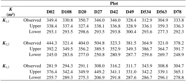
For each plot, a mixing proportion between 0 and 1 was found that maximized the stand 326

basal area increment. This mixing proportion varied between 38% and 74% depending on the 327

plot (Figure 3). 328

Figure 3 here 329

The difference between the optimum mixing proportion (xmax) and the mixing proportion

330

actually observed in the plots (xplot) varied from 0 to 34% (Table 4). The productivity gain

between these two proportions over the 6-year period was relatively low: 2.2% on average 332

with a maximum of 9% (Table 4). 333

Table 4 here 334

Although the elasticities of xmax to the parameters of the model varied from one plot to

335

another, a similar pattern was found across plots (Figure 4). The optimum mixing proportion 336

xmax was the most sensitive to the oak parameters, then to the pine parameters, then to the

337

inter-specific parameters. The parameters to which xmax was the most sensitive on average

338

were K1,1 and

λ1,1

. For K1,1 the elasticity is negative, meaning that an increase in K1,1 brings a

339

decrease in xmax. For

λ1,1

the elasticity is also negative but, as

λ1,1

is negative, it means that an

340

increase in

λ1,1

brings an increase in xmax. The parameter to which xmax was the least sensitive

341

on average was K1,2, with a positive or negative sign that varied depending on the focal plot.

342

From a quantitative point of view, a 1% increase in K1,1 (or a 1% decrease in

λ1,1

) led to a

343

decrease in xmax of between 1 and 1.2% while a 1% increase in K1,2 led to a variation in xmax of

344

between 0 and 0.2% depending on the plots. 345

The parameter K1,1 indicates the degree of aggregation of oaks. When K1,1 increases the

346

oaks are more aggregated and this leads to an increase in intra-specific competition.

λ1,1

is the

347

parameter that directly indicates the intensity of the intra-specific competition of oak because 348

it is associated to the competition index calculated on oak competitors. Since

λ1,1

is negative,

349

if this parameter decreases, it means that the intensity of the intra-specific competition 350

increases. We can therefore conclude that the optimum mixing proportion depends mainly on 351

the characteristics of the oak population and more particularly on parameters involved in the 352

intra-specific competition of oak (K1,1 and

λ1,1

).

4

Discussion

354

4.1 Complementarity between species

355

Our results suggest a positive effect of mixture on the productivity of oak-pine stands 356

(Figure 3). This result is consistent with those of Brown (1992) established for young oak-357

pine stands in an experimental design. Unlike Brown’s study (1992), we showed that, for 358

some mixing proportions, stand productivity reached a maximum; this indicates a situation of 359

"transgressive overyielding" (Figure 3). The gain between optimum productivity and current 360

productivity of the plots ranged from 0 to 9%. Our individual model was developed for 361

mixing proportions varying between 28% and 59%. Within this range, we can have 362

confidence in the stand model predictions. However, outside this range, and particularly for 363

extreme mixing proportions, the behaviour of the stand model is not guaranteed and may give 364

unrealistic predictions (see for example, plot D20 on Figure 3). The results obtained here 365

assume that the relationships fitted on mixed stands can be extrapolated to pure stands. 366

The effect of mixture on productivity is based on two main assumptions: "niche 367

complementarity" and "sampling effects" (Tilman et al. 2001). As we worked with only two 368

species and a variable mixing proportion, the "niche complementarity" hypothesis is more 369

likely to explain our findings. We studied a conifer-broadleaf forest with species having very 370

contrasting traits for light interception. Consequently, the complementarity of the two species 371

for the use of light is a strong hypothesis to explain a productivity increase in our mixed 372

stands (Ishii et al. 2004; Ishii and Asano 2010). Common oak is able to grow in the different 373

strata of the stand in contrast to Scots pine because oak is a more shade tolerant species than 374

Scots pine (Niinemets and Valladares 2006). Moreover, in our model there was a non-375

significant influence of oaks on pines (equation 2) probably because the pines had a greater 376

girth than oaks on average (Table 1). These two arguments may explain why a pure stand of 377

pine could be less productive than a pine stand where oaks were able to colonize the lower 378

strata. We also know that the light interception by the pine foliage is lower than the light 379

interception by the oak foliage (Balandier et al. 2006; Sonohat et al. 2004). This may help to 380

explain that in our oak model, the inter-specific competition was lower than the intra-specific 381

competition (equation 1) which contributes to a higher productivity in mixtures than in pure 382

stands of oak. The two species involved have different light requirements but also different 383

root distribution patterns (Brown 1992). The complementarity in nutrient and water use could 384

also contribute to a higher productivity in the mixture. The positive effect of mixture on stand 385

productivity that we found could thus be explained by spatial segregations in the aerial and 386

underground compartments. Our results concern the basal area productivity which does not 387

include differences in wood density of both species (Pretzsch 2005). To go further in the 388

study of the species complementarity, it would be interesting to estimate the effect of mixture 389

on biomass productivity. Further research is also necessary to identify the ecological 390

mechanisms that can explain the complementarity between these two species. 391

4.2 Over-yielding in mixed forests: a dynamic state

392

It is important to note that our models were developed from growth data corresponding to a 393

given time period (2000-2005). It is likely that the parameters of these models change with 394

time. For example, growth in juvenile Scots pine can be much faster than that of sessile oak 395

(Brown 1992) and it is possible that the ratio between intra- and inter-specific competition 396

changes over time for these species. This could explain why a situation of transgressive over-397

yielding could occur in mature stands and not in young stands. The impact of the temporal 398

dimension on our results can also be seen through the optimum mixing proportion formula. 399

Indeed, we calculated the optimum mixing proportion in the subspace of the state space 400

defined by known values for (G, r_G,1, r_G,2, r₁, r₂). This means that xmax can be considered as a

function of the state variables: xmax(G, rG,1, rG,2, r1, r2). As all these quantities, including the

402

mixing proportion itself, change with time, a pending question is whether 403

( )

max

(

( )

,G,1

( )

, G,2

( ) ( ) ( )

,1 , 2

)

x t =x G t r t r t r t r t (10)

404

at a given time ensures that 405

(

)

max

(

(

)

, G,1

(

)

, G,2

(

) (

,1

) (

, 2

)

)

x t+ ∆ =t x G t+ ∆t r t+ ∆t r t+ ∆t r t+ ∆t r t+ ∆t

406

at the subsequent time. There is actually no reason that this should be the case. This brings 407

up two questions: (1) Are there any initial values for (G, rG,1, rG,2, r1, r2) such that equation 10

408

would be verified at all times? (2) What type of silviculture - that is, an artificial modification 409

of N1 and N2 - would make it possible to verify equation 10 starting from arbitrary values for

410

(G, r_G,1, r_G,2, r₁, r₂)? The effect of mixture on stand productivity could be different for other

411

periods not only quantitatively but also qualitatively. Including the time factor in our results 412

will be the subject of future work. 413

4.3 Factors that influence the optimum mixing proportion

414

By simplifying and aggregating a distance-dependent individual-based model, we were 415

able to express the productivity of the stand as a function of the stand characteristics, the 416

model parameters and the mixing proportion (equation 8). Moreover, we have shown that it is 417

possible to explicitly express the optimum mixing proportion as a function of the mean 418

dendrometric characteristics of each species and the parameters of the individual model 419

(equation 9). After applying the stand model to the 9 plots in the study, our results showed 420

that there is some variability in the optimum value (Table 4). The optimum mixing proportion 421

(xmax) ranged from 38% to 74% of oak depending on the plot. We can explain this variability

422

among plots by studying the qualitative impact of the different factors on the optimum 423

provided by the local sensitivity analysis (Figure 4). For example the elasticity of xmax to the

424

spatial structure of oak (index K1,1) was negative. It means that the less aggregated the oaks

are, the fewer oaks there are within distance of 10 m on average, and consequently the more 426

their growth is promoted. The optimum then moves towards a stand where oak is more 427

represented. The same explanation can be used for pines and for the other factors. Finally, any 428

change in a factor that promotes the productivity of a species moves the optimum towards a 429

mixing proportion where the species is more represented. The local sensitivity analysis gave 430

us also quantitative results. For a given set of dendrometric characteristics, the optimum 431

mixing proportion was more sensitive to parameters involving oak - especially those 432

concerning its intra-specific competition (K1,1 et

λ1,1

) - than to those involving pine (Figure 4).

433

When the oak intra-specific competition increases, the optimum moves towards a stand with a 434

higher proportion of pine. In other words, the more intra-specific competition decreases 435

(decrease in K1,1 or increase in

λ1,1

), the more the optimum for productivity moves towards a

436

pure stand of oak. Our plots had different spatial patterns (Table 3) because they probably 437

experienced different ecological processes and different human actions (Ngo Bieng et al. 438

2006). As it has been recently shown for coexistence issues (see Hart and Marshall 2009), this 439

spatial structure has a direct impact on the optimum mixing proportion by changing intra and 440

inter-specific competition. 441

The mathematical equations that we developed can also inform us about the conditions 442

leading to a situation of over-yielding. For oak, the term

(

2 2

)

1,1K1,1 rG,1- 1,2K1,2 rG,2

λ λ is a

443

multiplicative factor for parameters a1 and b1 of the derivative of ∆G x1

( )

. Therefore, if

444

2 2

1,1K1,1 rG,1 1,2K1,2 rG,2

λ =λ the relationship between oak productivity and the mixing proportion is

445

a straight line which means that there would be no effect of mixture on oak productivity. In 446

the special case where we have the same average size for both sub-populations (rG,1=rG,2), a

447

random distribution of oaks and no spatial interaction between oak and pine ( 2

1,1 1,2 10

K =K =π ),

448

this condition corresponds to equality between intra-specific competition and inter-specific 449

competition (λ1,1 =λ1,2). The same result would have been achieved for pine if the parameter

450

2,1

λ had been different from zero when the individual model was fitted (section 2.2). This

451

finding is consistent with a known theoretical result: for two species A and B growing in a 452

mixture, if the effect of A on B is the same as that of B on B and if the effect of B on A is the 453

same as that of A on A, then the productivity of a species in a mixture is the product of its 454

proportion by its productivity in a pure stand (Harper 1977). In this case, the relationships 455

between the productivity of species and the mixing proportion are straight lines (left side of 456

Figure 1). However, our results also show that spatial structure and average size of sub-457

populations play a role in the conditions leading to over-yielding. This complements the 458

results obtained from the Lokta-Volterra theoretical model of inter-specific competition 459

(Loreau 2004). This means that, in the case of our two-species mixed forest, the condition 460

"intra-specific competition greater than inter-specific competition" is not sufficient to ensure 461

over-yielding. 462

5

Conclusion

463

Our results show that mixture has a positive effect on the productivity of oak-pine stands 464

and that transgressive over-yielding can occur in these stands. These findings indicate good 465

complementarity between these two species. Our modelling-based approach allowed us to 466

express the optimum mixing proportion as a function of stand characteristics and parameters 467

from a distance-dependent individual-based model. We showed that, for a given set of 468

dendrometric characteristics, the optimum mixing proportion depends mainly on parameters 469

involving the oak species, and especially those concerning its intra-specific competition. 470

However, the mathematical equation for the optimum mixing proportion indicated that an 471

intra-specific competition higher than inter-specific competition was not a sufficient condition 472

to ensure over-yielding. We also showed how to use results obtained at the individual level to 473

obtain results on the behaviour of the whole system. As part of the issue on productivity in 474

mixed forests, this kind of approach can help us to better understand the link between 475

productivity, stand characteristics and growth parameters of species. 476

Acknowledgements

477

This work forms part of the PhD traineeship of T. Perot and was funded in part by the 478

research department of the French National Forest Office. We are grateful to the Loiret 479

agency of the National Forest Office for allowing us to install the experimental sites in the 480

Orleans state forest. Many thanks to the Cemagref staff at Nogent-sur-Vernisson who helped 481

collect the data. 482

References

483

Balandier P., Sonohat G., Sinoquet H., Varlet-Grancher C., Dumas Y. (2006) 484

Characterisation, prediction and relationships between different wavebands of solar 485

radiation transmitted in the understorey of even-aged oak (Quercus petraea, Q-robur) 486

stands. Trees-Structure and Function 20: 363-370. 487

Biging GS, Dobbertin M (1992) A comparison of distance-dependent competition measures 488

for height and basal area growth of individual conifer trees. Forest Science 38:695-720 489

Brown AHF (1992) Functioning of mixed-species stands at Gisburn, N.W. England. In: 490

Cannell MGR, Malcolm DC, Robertson PA (eds) The ecology of mixed-species stands 491

of trees. Blackwell scientific publications, Oxford, pp 125-150 492

Canham CD, LePage PT, Coates KD (2004) A neighborhood analysis of canopy tree 493

competition: effects of shading versus crowding. Canadian Journal of Forest Research 494

34:778-787 495

Cressie NAC (1993) Statistics for spatial data. John Wiley and sons, New York 496

de Wit CT (1960) On competition. Institute for biological and chemical research on field 497

crops and herbage, Wageningen 498

del Rio M, Sterba H (2009) Comparing volume growth in pure and mixed stands of Pinus 499

sylvestris and Quercus pyrenaica. Annals of Forest Science 66:502p501-502p511 500

Dieckmann U, Law R, Metz JAJ (2000) The Geometry of Ecological Interactions: 501

Simplifying Spatial Complexity. Cambridge University Press, Cambridge 502

Garber SM, Maguire DA (2004) Stand productivity and development in two mixed-species 503

spacing trials in the central Oregon cascades. Forest Science 50:92-105 504

Harper JL (1977) Population biology of plants. Academic Press, London 505

Hart SP, Marshall DJ (2009) Spatial arrangement affects population dynamics and 506

competition independent of community composition. Ecology 90:1485-1491 507

Hector A (2006) Overyielding and stable species coexistence. New Phytologist 172:1-3 508

Hector A, Bazeley-White E, Loreau M, Otway S, Schmid B (2002) Overyielding in grassland 509

communities: testing the sampling effect hypothesis with replicated biodiversity 510

experiments. Ecology Letters 5:502-511 511

Hector A et al. (1999) Plant diversity and productivity experiments in European grasslands. 512

Science 286:1123-1127 513

Hooper DU et al. (2005) Effects of biodiversity on ecosystem functioning: A consensus of 514

current knowledge. Ecological Monographs 75:3-35 515

Illian J, Penttinen A, Stoyan H, Stoyan D (2008) Statistical Analysis and Modelling of Spatial 516

Point Patterns. Wiley, Chichester 517

Ishii H, Asano S (2010) The role of crown architecture, leaf phenology and photosynthetic 518

activity in promoting complementary use of light among coexisting species in temperate 519

forests. Ecological Research 25:715-722 520

Ishii HT, Tanabe S, Hiura T (2004) Exploring the relationships among canopy structure, stand 521

productivity, and biodiversity of temperature forest ecosystems. Forest Science 50:342-522

355 523

Jolliffe PA (2000) The replacement series. Journal of Ecology 88:371-385 524

Kelty MJ (2006) The role of species mixtures in plantation forestry. Improving Productivity 525

in Mixed-Species Plantations. Forest Ecology and Management 233:195-204 526

Kelty MJ, Larson BC (1992) The ecology of silviculture of mixed species forest. Kluwer 527

Academic Publishers, Dordrecht 528

Levin SA, Pacala SW (1997) Theories of simplification and scaling of spatially distributed 529

processes. In: Tilman D, Kareiva P (eds) Spatial Ecology: The Role of Space in 530

Population Dynamics and Interspecific Interactions. Princeton University Press, 531

Princeton, p 271–295 532

Loreau M (2004) Does functional redundancy exist? Oikos 104:606-611 533

Loreau M, Naeem S, Inchausti P (2002) Biodiversity and ecosystem functioning : synthesis 534

and perspectives. Oxford university press, Oxford 535

Loreau M et al. (2001) Ecology - Biodiversity and ecosystem functioning: Current knowledge 536

and future challenges. Science 294:804-808 537

Lotwick HW, Silverman BW (1982) Methods for analysing spatial processes of several types 538

of points. Journal of the Royal Statistical Society B 44:406-413 539

Luis JFS, Monteiro MD (1998) Dynamics of a broadleaved (Castanea sativa) conifer 540

(Pseudotsuga menziesii) mixed stands in Northern Portugal. Forest Ecology and 541

Management 107:183-190 542

MCPFE, UNECE, FAO (2007) State of Europe's forests 2007. MCPFE, Warsaw 543

Morneau F, Duprez C, Hervé JC (2008) Les forêts mélangées en France métropolotaine. 544

Caractérisation à partir des résultats de l'Inventaire Forestier National. Revue Forestiere 545

Francaise LX:107-120 546

Ngo Bieng MA, Ginisty C, Goreaud F, Perot T (2006) A first typology of Oak and Scots pine 547

mixed stands in the Orleans forest (France), based on the canopy spatial structure. New 548

Zealand Journal of Forestry Science 36:325-346 549

Niinemets U, Valladares F (2006) Tolerance to shade, drought, and waterlogging of temperate 550

Northern Hemisphere trees and shrubs. Ecological Monographs 76:521-547 551

Perot T, Goreaud F, Ginisty C, Dhote JF (2010) A model bridging distance-dependent and 552

distance-independent tree models to simulate the growth of mixed forests. Annals of 553

Forest Science 67:502p1-502p11 554

Picard N, Franc A (2001) Aggregation of an individual-based space-dependent model of 555

forest dynamics into distribution-based and space-independent models. Ecological 556

Modelling 145:69-84 557

Piotto D (2008) A meta-analysis comparing tree growth in monocultures and mixed 558

plantations. Forest Ecology and Management 255:781-786 559

Pretzsch H (2005) Diversity and productivity in forests: Evidence from long-term 560

experimental plots. Forest Diversity and Function: Temperate and Boreal Systems 561

176:41-64 562

Pretzsch H (2009) Forest dynamics, growth and yield: from measurement to model, Springer, 563

Berlin Heidelberg 564

Pretzsch H, Schutze G (2009) Transgressive overyielding in mixed compared with pure 565

stands of Norway spruce and European beech in Central Europe: evidence on stand 566

level and explanation on individual tree level. European Journal of Forest Research 567

128:183-204 568

Ripley BD (1977) Modelling spatial patterns. Journal of the royal statistical society B 39:172-569

212 570

Schmid B, Hector A, Saha P, Loreau M (2008) Biodiversity effects and transgressive 571

overyielding. Journal of Plant Ecology-Uk 1:95-102 572

Sonohat G., Balandier P., Ruchaud F. (2004) Predicting solar radiation transmittance in the 573

understory of even-aged coniferous stands in temperate forests. Annals of Forest 574

Science 61: 629-641 575

Stadt KJ, Huston C, Coates KD, Feng Z, Dale MRT, Lieffers VJ (2007) Evaluation of 576

competition and light estimation indices for predicting diameter growth in mature boreal 577

mixed forests. Annals of Forest Science 64:477-490 578

Thebault E, Loreau M (2006) The relationship between biodiversity and ecosystem 579

functioning in food webs. Ecological Research 21:17-25 580

Tilman D, Reich PB, Knops J, Wedin D, Mielke T, Lehman C (2001) Diversity and 581

productivity in a long-term grassland experiment. Science 294:843-845 582

Uriarte M, Condit R, Canham CD, Hubbell SP (2004) A spatially explicit model of sapling 583

growth in a tropical forest: does the identity of neighbours matter? Journal of Ecology 584

92:348-360 585

Vandermeer J (1989) The ecology of intercropping. Cambridge University Press, Cambridge 586

Vila M, Vayreda J, Comas L, Ibanez JJ, Mata T, Obon B (2007) Species richness and wood 587

production: a positive association in Mediterranean forests. Ecology Letters 10:241-250 588

Tables

590

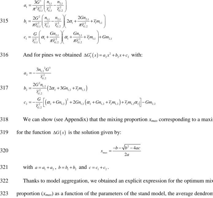
591

Table 1. Dendrometric characteristics of the plots. S = plot area; r_G,1 = quadratic mean radius for oak; r_G,2 =

592

quadratic mean radius for pine; r = mean radius for oak; ₁ r = mean radius for pine; (sd) = standart deviation; N₂ 1

593

= number of oaks per hectare; N2 = number of pines per hectare; G1 = oak basal area per hectare; G2 = pine basal

594

area per hectare.

595 Plot S (ha) ,1 G r (cm) ,2 G r (cm) 1 r (sd) (cm) 2 r (sd) (cm) N1 (trees.ha-1) N2 (trees.ha-1) G1 (m².ha-1) G2 (m².ha-1) D02 0.951 11.1 17.7 10.0 (4.9) 17.3 (3.5) 354.3 96.7 13.8 9.5 D108 0.800 8.5 16.9 8.0 (3.0) 16.7 (2.6) 353.8 231.3 8.1 20.8 D20 1.015 8.1 16.2 7.5 (3.0) 15.9 (3.1) 481.7 162.5 9.9 13.4 D27 0.625 8.2 17.7 7.3 (3.6) 17.3 (3.8) 396.8 128.0 8.3 12.6 D42 0.500 8.2 12.5 7.7 (2.8) 12.0 (3.5) 472.0 280.0 9.8 13.6 D49 0.994 8.7 15.2 8.0 (3.5) 14.8 (3.1) 493.0 237.4 11.8 17.2 D534 0.500 8.2 18.1 7.6 (3.0) 17.9 (3.1) 488.0 170.0 10.2 17.6 D563 0.500 12.3 16.2 11.4 (4.6) 16.1 (2.2) 242.0 212.0 11.4 17.4 D78 0.700 9.7 20.9 9.1 (3.2) 20.5 (4.1) 407.1 112.9 12.0 15.6 596

Table 2. Parameter estimates for the distance-dependent individual-based model (equations 1 and 2). 597 Oak Pine Plot ααααk,1 (mm) ββββk,1 (mm.cm-1) λλλλ1,1 (mm) λλλλ1,2 (mm) αααα2 (mm) ββββk,2 (mm.cm-1) λλλλ2,2 (mm.cm-2) D02 5.99 0.1026 -0.354 -0.242 4.60 0.0566 -0.000361 D108 12.08 0.0896 -0.354 -0.242 4.60 0.0620 -0.000361 D20 12.45 0.0427 -0.354 -0.242 4.60 0.0633 -0.000361 D27 12.73 0.0361 -0.354 -0.242 4.60 0.0512 -0.000361 D42 9.62 0.1633 -0.354 -0.242 4.60 0.0813 -0.000361 D49 13.01 0.0600 -0.354 -0.242 4.60 0.0511 -0.000361 D534 7.73 0.1357 -0.354 -0.242 4.60 0.0476 -0.000361 D563 6.00 0.1066 -0.354 -0.242 4.60 0.0491 -0.000361 D78 4.00 0.1766 -0.354 -0.242 4.60 0.0337 -0.000361 598 599 600

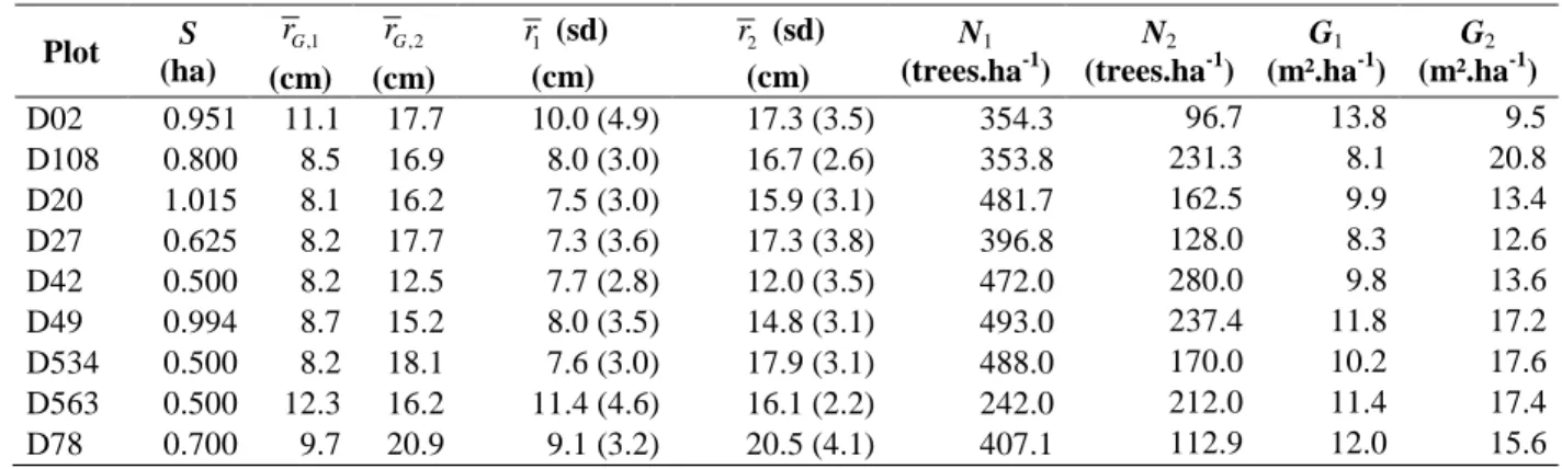
Table 3. Values of the Ripley's function for oak (K1,1) and for pine (K2,2), and values of the inter-type function

601

(K1,2) at a distance of 10 m in each plot. The 99% confidence limits under the null hypothesis are also given

602

(upper and lower bounds). For the Ripley’s function, the null hypothesis corresponds to complete spatial

603

randomness. For the inter-type function, the null hypothesis corresponds to population independence.

604 Plot K (m²) D02 D108 D20 D27 D42 D49 D534 D563 D78 K1,1 Observed 349.4 330.8 350.7 346.0 346.0 328.4 312.9 304.9 333.8 Upper 338.4 337.4 327.4 338.1 336.8 328.9 336.1 359.3 336.3 Lower 293.1 293.5 298.6 293.5 293.8 300.4 293.6 277.3 292.3 K2,2 Observed 444.3 321.4 404.0 504.8 323.3 381.5 364.9 321.0 378.2 Upper 392.2 349.5 356.2 389.5 352.9 349.3 386.7 364.7 391.7 Lower 245.0 283.6 277.0 250.8 280.9 287.7 259.6 269.7 248.9 K1,2 Observed 281.9 294.3 291.1 308.0 316.2 311.7 343.9 308.8 304.7 Upper 376.4 342.4 349.9 449.2 341.1 331.0 342.2 339.1 365.1 Lower 255.7 289.3 275.3 206.9 291.8 287.6 286.7 296.1 278.8 605

Table 4. Optimum mixing proportion (xmax) and observed mixing proportion (xplot) for each plot; ∆G(xmax) = 606

stand basal area increment for x = xmax; ∆G(xplot) = stand basal area increment for x = xplot; Gain = relative

607

difference between ∆G(xmax) and ∆G(xplot).

608 Plot xmax (%) ∆∆∆∆G(xmax) (m²/ha/an) xplot. (%) ∆∆∆∆G(xplot) (m²/ha/an) Gain (%) D02 59.3 0.477 59.2 0.477 0.00 D108 43.1 0.591 28.0 0.561 4.91 D20 37.5 0.555 42.6 0.552 0.61 D27 46.5 0.295 39.8 0.292 0.96 D42 45.7 0.374 41.9 0.373 0.21 D49 46.2 0.647 40.8 0.642 0.64 D534 40.8 0.291 36.7 0.290 0.40 D563 73.6 0.320 39.6 0.291 9.05 D78 57.3 0.401 43.6 0.387 3.41 609

Figure captions

610

611

Figure 1. The three main types of productivity response for a mixed stand composed of two species A and B

612

according to the mixing proportion (adapted from Harper, 1977). Total density is assumed to be constant for the

613

different mixing proportions. On the left, mixture has no effect on stand productivity: productivity of mixed

614

stands is equivalent to the juxtaposition of pure stands. In the middle, mixture has a negative effect on stand

615

productivity: productivity of mixed stands is lower than the productivity expected in juxtaposed pure stands. On

616

the right, mixture has a positive effect on stand productivity: productivity of mixed stands is higher than the

617

productivity expected in juxtaposed pure stands.

618 619

Figure 2. Comparison between the distance-dependent individual-based model and the stand model for oak (a)

620

and pine (b) and for the 9 plots. Basal Area Increment = stand basal area increment predicted by the models over

621

the 2000-2005 period. Individual model: distance-dependent individual-based model (equations 1 and 2). Stand

622

model: stand model obtained by aggregation of the individual model (equation 7).

623 624

Figure 3. Stand productivity according to the mixing proportion for the 9 plots and for each species. The solid

625

curve represents total stand productivity. The curve with black dots represents pine productivity. The curve with

626

white dots represents oak productivity. The dashed vertical line represents the mixing proportion observed in the

627

plot (xplot). The solid vertical line represents the optimum mixing proportion (xmax).

628 629

Figure 4. Elasticiticies of xmax to the 10 parameters of the stand model for each plot. The bars show the absolute

630

values of the elasticities, the sign of the elasticities being written on top of each bar.

631 632

Figures

633 Proportion of species A P ro d u c ti v it y 0.0 0.5 1.0 A+B A B Proportion of species A P ro d u c ti v it y 0.0 0.5 1.0 A+B A B Proportion of species A P ro d u c ti v it y 0.0 0.5 1.0 A+B A B 634 635 Figure 1 636 637

638 D02 D108 D20 D27 D42 D49 D534 D563 D78 Oak Plot B a s a l A re a I n c re m e n t (m ²/ h a ) 0 .0 0 .5 1 .0 1 .5 2 .0 2 .5 3 .0 Individual model Stand model (a) 639 D02 D108 D20 D27 D42 D49 D534 D563 D78 Pine Plot B a s a l A re a I n c re m e n t (m ²/ h a ) 0 .0 0 .5 1 .0 1 .5 2 .0 2 .5 3 .0 Individual model Stand model (b) 640 641 Figure 2 642 643

644 x (oak proportion) P ro d u c ti v it y ( m ²/ h a /a n ) 0.2 0.4 0.6 0.8 0.0 0.2 0.4 0.6 0.8 1.0 D02 D108 0.0 0.2 0.4 0.6 0.8 1.0 D20 D27 D42 0.2 0.4 0.6 0.8 D49 0.2 0.4 0.6 0.8 D534 0.0 0.2 0.4 0.6 0.8 1.0 D563 D78 645 646 Figure 3 647 648

649 0 0.2 0.4 0.6 0.8 1 1.2 Elasticity of xm a x Koak, oak λoak, oak αoak βoak βpine αpine λpine, pine Kpine, pine λoak, pine Koak, pine D02 D108 D20 D27 D42 D49 D534 D563 D78 650 651 Figure 4 652

Appendix

653

Aggregating the distance-independent individual-based model 654

Given a distance-independent individual-based model: 655 , , i j j j i j r γ β girth ∆ = + (11) 656

where ∆ri,j is the radial increment of a tree i belonging to a species j between time t and

657

time t+∆t, girthi,j is the girth at time t for a tree i. Starting from equation 11, we can develop a

658

stand model for species j using an aggregation approach. The stand can be defined with three 659

aggregated variables for each species: the number of trees Nj, the mean radius rj and the basal

660

area Gj. The dynamic equations of these variables must be defined using equation 11. Since

661

we assume that there is neither mortality nor recruitment between t and t+∆t, we have 662

0 j N

∆ = . The mean radius is defined as follows:

663

( )

, 1 1 Nj j i j i j r t r N = =

∑

664

where r tj

( )

is the mean radius at time t. The mean radius increment can thus be written as

665

a function of the individual radial increments: 666

(

)

( )

,

(

)

,

( )

, 1 1 1 1 Nj 1 Nj 1 Nj j j j i j i j i j i i i j j j r r t t r t r t t r t r N = N = N = ∆ = + ∆ − =

∑

+ ∆ −

∑

=

∑

∆ 667

It follows from equation 11 that: 668 , 1 2 j N i j j j j j j i r γ N πβ N r = ∆ = +

∑

669

And the mean radius increment is given by: 670 2 j j j j r γ πβ r ∆ = + 671

Similarly, ∆Gj can be written as a function of the individual basal area increments (∆gi j, ):

672

(

)

( )

,

(

)

,

( )

, 1 1 1 j j j i N i N i N j i j i j i j i i i G G t t G t g t t g t g = = = = = = ∆ = + ∆ − =

∑

+ ∆ −

∑

=

∑

∆ 673