Global ozone forecasting based on ERS-2 GOME observations

HAL Id: hal-00295205

https://hal.archives-ouvertes.fr/hal-00295205

Submitted on 28 Oct 2002

HAL is a multi-disciplinary open access

archive for the deposit and dissemination of

sci-entific research documents, whether they are

pub-lished or not. The documents may come from

teaching and research institutions in France or

abroad, or from public or private research centers.

L’archive ouverte pluridisciplinaire HAL, est

destinée au dépôt et à la diffusion de documents

scientifiques de niveau recherche, publiés ou non,

émanant des établissements d’enseignement et de

recherche français ou étrangers, des laboratoires

publics ou privés.

Global ozone forecasting based on ERS-2 GOME

observations

H. J. Eskes, P. F. J. van Velthoven, H. M. Kelder

To cite this version:

H. J. Eskes, P. F. J. van Velthoven, H. M. Kelder. Global ozone forecasting based on ERS-2 GOME

observations. Atmospheric Chemistry and Physics, European Geosciences Union, 2002, 2 (4),

pp.271-278. �hal-00295205�

www.atmos-chem-phys.org/acp/2/271/

Chemistry

and Physics

Global ozone forecasting based on ERS-2 GOME observations

Royal Netherlands Meteorological Institute, De Bilt, The Netherlands

Received: 4 June 2002 – Published in Atmos. Chem. Phys. Discuss.: 10 July 2002 Revised: 10 October 2002 – Accepted: 14 October 2002 – Published: 28 October 2002

Abstract. The availability of near-real time ozone

observa-tions from satellite instruments has recently initiated the de-velopment of ozone data assimilation systems. In this paper we present the results of an ozone assimilation and forecast-ing system, in use since Autumn 2000. The forecasts are produced by an ozone transport and chemistry model, driven by the operational medium range forecasts of ECMWF. The forecasts are initialised with realistic ozone distributions, tained by the assimilation of near-real time total column ob-servations of the GOME spectrometer on ERS-2. The fore-cast error diagnostics demonstrate that the system produces meaningful total ozone forecasts for up to 6 days in the ex-tratropics. In the tropics meaningful forecasts of the small anomalies are restricted to shorter periods of about two days with the present model setup. It is demonstrated that impor-tant events, such as the breakup of the South Pole ozone hole and mini-hole events above Europe can be successfully pre-dicted 4–5 days in advance.

1 Introduction

Data assimilation is a well established essential component in numerical weather prediction. Based on the available ob-servations from satellite, balloon sounding, aircraft and other sources, and based on the model forecast, the most probable state of the atmosphere is constructed. This analysis is sub-sequently used as the starting point for a weather forecast.

The application of data assimilation in the field of atmo-spheric chemistry research is still very new. This develop-ment was motivated by the experiences of numerical weather prediction centres, as well as by the availability of global data sets on ozone and other chemical species from satellite in-struments. New satellite missions such as Envisat and EOS-Aura will provide huge volumes of detailed observations of

Correspondence to: H. J. Eskes (eskes@knmi.nl)

the 3-D composition of the atmosphere. Data assimilation will play an important role to make optimal use of these fu-ture data sets.

A realistic forecast or simulation of the chemical state of the atmosphere depends on the quality of the model (the description of atmospheric transport and the chemical reac-tions) but also on the initial conditions (concentrations of es-pecially long lived chemical species) and sources and sinks. Data assimilation uses the available data in an objective way to fix the initial state. This provides a means to study the quality of the chemistry scheme and description of advec-tion and convecadvec-tion in the model. For instance, Fisher and Lary (1995) have shown how a 4-D-Var variational assimila-tion of a few chemical observaassimila-tions can provide strong con-straints on a chemical model with an extensive set of species. This work has inspired several recent assimilation studies on stratospheric and tropospheric chemistry (see, for instance, Khattatov et al., 2000).

Ozone is an important trace gas for numerical weather forecast modelling. Because of the strong absorption of ul-traviolet and infrared radiation, ozone has a strong influ-ence on the temperature and the dynamics in the atmosphere. A knowledge of ozone may improve satellite retrievals, es-pecially the radiation modelling for the TOVS instruments. Furthermore, the assimilation of ozone observations in a modern 4-D-Var or Kalman filter approach will have a di-rect impact on the wind field (Riishøjgaard, 1996). In the pioneering European Union project Satellite Ozone Data As-similation (Stoffelen et al., 1999), http://www.knmi. nl/soda/, techniques have been developed for the assimi-lation of ozone in several numerical weather forecast models, including the European Centre for Medium Range Weather Forecast (ECMWF) model. ECMWF ozone forecasts, based on near-real time satellite ozone data, are available from April 2002. The National Oceanic and Atmospheric Admin-istration (NOAA) has recently started to provide ozone fore-casts based on assimilated operational Solar Backscatter UV

272 H. J. Eskes et al.: Global ozone forecasting

(SBUV/2) data from the NOAA satellites. The Data Assim-ilation Office of NASA has developed the GEOS ozone data assimilation system for the off-line analysis of Total Ozone Mapping Spectrometer (TOMS) and SBUV/2 data ( ˘Stajner et al., 2001). The University of Reading, in collaboration with the UK Met Office, has developed an ozone data as-similation system for MLS and GOME ozone data (Struthers et al., 2002).

These activities can be seen as a first step toward a chemi-cal forecasting system that is based on an assimilated chem-ical analysis. In the past years, chemchem-ical transport model runs based on meteorological forecasts have proved to be very useful during measurement campaigns (Lee et al., 1997; Flatøy et al., 2000) as a tool for measurement planning and interpretation.

In this paper we describe the quantitative results of an operational ozone assimilation and forecasting system de-veloped at the Royal Netherlands Meteorological Institute (KNMI). The system is based on GOME ozone data and a chemistry transport model driven by ECMWF forecasts of the meteorological fields. Daily ozone forecasts, and a data base of ozone fields is provided via the web site of the KNMI,http://www.knmi.nl/gome_fd(Van der A et al., 2000). First, the assimilation analysis, based on GOME ozone observations, will be briefly discussed. Then the ozone forecast scores will be presented. The last section discusses two interesting examples, namely the breakup of the ozone hole and a recent ozone mini-hole over Europe.

2 The model

The ozone forecasts are based on a tracer-transport and as-similation model called TM3-DAM. The modelling of the transport, chemistry and the aspects of the ozone data assim-ilation are described in detail in a recent paper (Eskes et al., 2002). Here we will only provide a brief overview of the model setup.

2.1 Transport

The three-dimensional advection of ozone is described by the flux-based second order moments scheme of Prather (1986). The model follows the new ECMWF vertical layer defini-tion, operational from the end of 1999 until the present. The 60 ECMWF hybrid layers between 0.1 hPa and the surface have been reduced to 44 in TM3-DAM by removing 16 lay-ers in the lower and middle troposphere. Above 300 hPa the layers in the model coincide with the ECMWF layers. The horizontal resolution of the model version used in this study is 2.5 by 2.5 degree.

The model is driven by 6-hourly meteorological fields (wind, surface pressure, temperature) from the ECMWF model. TM3-DAM is used in diagnostic and forecast mode. The diagnostic mode is driven by the archived six hour

fore-cast (ECMWF first guess) fields. In forefore-cast mode the model is driven by the results of the latest forecast run performed at the ECMWF. In both modes the meteorological fields are updated every 6 hours.

2.2 Chemistry

Ozone chemistry is described by two parameterisations. One follows the work of Cariolle and D´equ´e (1986) and consists of a linearisation of the chemistry with respect to sources and sinks, the ozone amount, temperature and UV radia-tion. The Cariolle scheme is also used by other groups in-volved in ozone data assimilation and/or forecasting, namely the ECMWF and the Data Assimilation Research Centre at Reading (Struthers et al., 2002). A second parametrisation scheme accounts for heterogeneous ozone loss (P. Braesicke, private communications). This scheme introduces a three-dimensional chlorine activation tracer which is formed when the temperature drops below the critical temperature of polar stratospheric cloud formation. Ozone breakdown occurs in the presence of the activation tracer. We performed model runs without assimilation for the period July–September 2000, and found that the chemistry parameterisations provide a realistic simulation of the formation of the 2000 ozone hole. The motivation for using chemistry parameterisations is, first of all, to reduce the computational cost. Secondly, the largest changes in ozone on the time scale of one day to a week are related mainly to transport. Even the dramatic ozone break-down occurring at the South Pole in August–September has a time scale of a week to a month. This should be compared with the 1 to 3 days within which new GOME measurements become available to the assimilation. The parametrisations remove a large part of the bias the model would have with-out any chemistry, and ensure that the ozone profile shape remains realistic.

2.3 Observations

The ozone analysis is based on total column ozone observa-tions measured by the GOME instrument, part of the payload of the ERS-2 satellite of ESA. A discussion of the ozone products and retrieval techniques can be found in Burrows et al. (1999). For ozone forecasting purposes a near-real time product is essential. The data assimilation results described here are based on the fast delivery total ozone columns (Valks et al., 2002). The GOME measurements are collected and ozone columns are retrieved within 3 h after the measure-ments are made. The width of the GOME swath is 960 km, divided in three pixels of 320 by 40 km, and the number of total ozone observations is about 18.000 per day. GOME has a global coverage in three days (apart from the dark winter pole).

2.4 Assimilation approach

The total ozone data is assimilated in TM3-DAM based on a parametrised Kalman filter technique. In this approach the forecast error covariance matrix is written as a product of a time independent correlation matrix and a time-dependent di-agonal variance. The various parameters in the approach are fixed based on the forecast minus observation statistics accu-mulated over the period of one year (2000). This approach produces detailed and realistic time- and space-dependent forecast error distributions. Several aspects of the error mod-elling approach have been discussed before in Eskes et al. (2002), and Jeuken et al. (1999).

2.5 Assimilation results

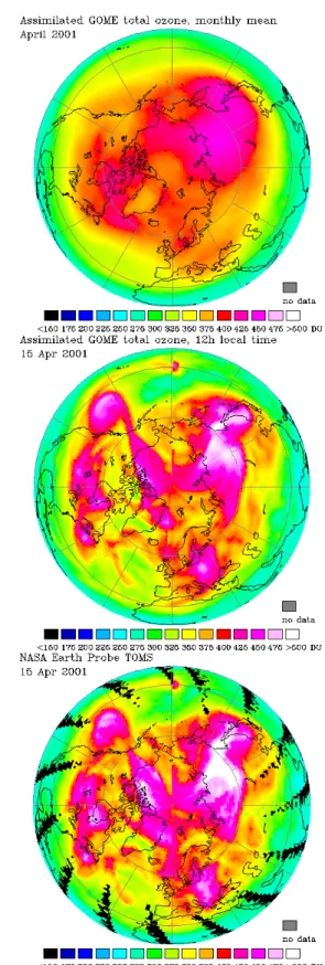
An example of the ozone analyses produced in this way is shown in Fig. 1, second panel. For comparison, we show an Earth Probe TOMS (McPeters et al., 1998) map of ozone on 15 April 2001 in the third panel. TOMS has a nearly global coverage in one day, and the figure shows the ozone column observations gridded on a 1 by 1.25 degree grid. Because TOMS has a sun-synchronous orbit, we have constructed a 12 h local time global ozone map based on the model analysis (second panel). The date line is clearly visible at 180 degree longitude in both frames.

As is clear from the figure, the agreement between TOMS and the TM3-DAM assimilated GOME field is good. The small-scale features in ozone correlate very well with the small scale features in the TOMS map. The image pro-vides an impression of the amount of detail in the assimilated ozone fields and the effective resolution of the model. On a larger scale there are also clear differences. This larger-scale offset between the two plots can for a large part be attributed to differences in the instruments and the retrieval codes for TOMS and GOME total ozone.

The observation minus forecast statistics is discussed in more detail in Eskes et al. (2002). On average the root-mean-square (RMS) observation-minus-forecast difference between GOME observations (before assimilation) and the short range model forecast (between 1 and 3 days) is small: about 9 Dobson Units (DU), or roughly 3%. The distribu-tion of RMS differences is well approximated by a Gaussian curve, which is consistent with the Kalman filter assumption that both the observation and forecast have Gaussian random errors. The bias between the model forecast and the GOME ozone columns is in general smaller than 1%, a factor of 3–10 smaller than the RMS. Because of this, no additional bias corrections are applied to the forecast model. The small bias implies that the assimilation efficiently adopts the ozone levels as retrieved from the GOME spectra. Note that this small bias does not imply that the GOME data themselves have a similar small bias. In general the comparison between the GOME fast-delivery retrieval and ground-based observa-tions is within 5% for low- and midlatitudes, and within 10%

Fig. 1. Total ozone distribution in the Northern hemisphere in April

2001. Top: monthly mean. Centre: Analysis on 15 April, 12:00 LT. Bottom: Earth Probe TOMS observations for 15 April. Scales in Dobson units.

274 H. J. Eskes et al.: Global ozone forecasting

at high latitudes and high solar zenith angles (Valks et al., 2002).

2.6 Operational ozone forecasts

Every day two forecast runs are performed. Directly af-ter completion of the 10-day ECMWF forecast (started at 12:00 UTC) the meteorological fields are extracted from the archive. The wind fields are converted into mass fluxes in a preprocessing step, and the data is sent to KNMI. Upon ar-rival an analysis and forecast run is started at KNMI, based on the latest near-real time GOME ozone data. Twelve hours later a new forecast run is performed, based on the same meteorological fields, but with an additional 12 h of GOME measurements. The forecast statistics discussed below are accumulated for the first forecast run only.

3 Anomaly correlation and RMS error

In numerical weather prediction it is common practice to measure the performance of the medium-range forecast by plotting the anomaly correlation Ct. Typically anomalies of

the 500 hPa height field are monitored (or wind field anoma-lies in the tropics) (Simmons et al., 1995). In this paper we will investigate variations in the total column of ozone. The anomaly correlation is usually defined as,

Ct =

(ft−c)(a − c)

q

(ft−c)2(a − c)2

(1)

Here c is the climatological total ozone value, i.e. the aver-age over many years of a particular month or day, for a par-ticular latitude and longitude. ft is the forecast which was

produced at time t before the verifying analysis a. Ct

mea-sures the correlation between the forecast anomaly (ft −c)

with a forecast time t and the analysis anomaly (a − c), both applying to the same time. The average is over forecast runs and over latitude/longitude.

The anomaly correlation in this form is not a very useful quantity for total ozone (see, for instance, D´equ´e (1997) for a discussion of problems related to the anomaly correlation score). An important assumption in Eq. (1) is that the cli-matological mean is well defined, and that (a − c) → 0 for long averaging periods. This is not the case for ozone: there are considerable trends related to ozone depletion, there is a strong seasonal variation and a considerable year to year vari-ation. Equation (1), evaluated based on, e.g. a 20 year clima-tology, will provide a too optimistic estimate of the forecast performance: persistent differences with respect to climatol-ogy will tend to inflate Ct.

The first panel of Fig. 1 shows the monthly-mean ozone distribution for April 2001. Note that there is a pronounced zonal variation (with pronounced wave 1 and wave 2 com-ponents). The monthly mean ozone maps also show a strong variability from year to year, e.g. the Northern Hemisphere

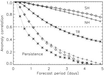
Fig. 2. Modified anomaly correlation as a function of the forecast

period. The top three curves represent the total ozone anomaly for latitudes north of 30 degree (NH), between −30 and 30 degree (TR) and south of −30 degree (SH). The lower three curves are the cor-responding scores for persistence.

ozone amount in April 2000 was about 20 DU lower than in 2001. Motivated by this, we introduce a modified anomaly correlation C(m)_t in which the anomalies are computed as the difference between the actual ozone column and a centred monthly mean, i.e. the anomalies as defined as the differ-ences between the second and first panel in Fig. 1.

Figure 2 shows the modified anomaly correlation as a function of the forecast time. The plot is based on approx-imately 9 months of forecast runs between December 2000 and January 2002. The top three curves correspond to the extratropical northern hemisphere (NH), the tropics (TR) and the extratropical southern hemisphere (SH). For comparison we also show the results for persistence (dotted curves). Per-sistence is calculated by keeping ozone fixed during the fore-cast period. Clearly the forefore-cast runs are superior to persis-tence, which is only meaningful for a short time interval of about 1 day, when the anomaly drops below 0.6. We have also produced plots for the individual months, which all pro-vide a very comparable behaviour to Fig. 2, although there is some variation from one month to another.

The SH and NH curves are an encouraging result: after 5 days the forecast anomaly correlation is still well above 0.6. Extrapolation suggests that on average the forecasts are meaningful up to 6–7 days. The current ECMWF meteoro-logical forecasts are characterised by 500 hPa geopotential height anomalies that cross 0.6 after about 7 days, which is quite comparable to what we find for total ozone. Note that this crossing time is sensitive to the choice of the climatolog-ical reference c (in our case a running monthly mean), and this dependence is one of the factors which complicates the direct comparison between the total ozone and height anoma-lies.

The plot also suggests that the southern hemisphere has a slightly better score than the northern hemisphere. This may seem a bit surprising. Traditionally the forecast skill of nu-merical weather prediction models has been better in the NH related to the dense observation network. In recent years this difference between the hemispheres in the ECMWF model has disappeared, and both sectors show good forecast skill up to 7 days (Lalaurette and Ferranti, 2001). In the plots for the individual months there is a considerable spread in the comparison between NH and SH, ranging from C_t(m) in the SH being slightly lower than SH, to significantly higher (e.g. October 2001). A longer forecast data set is needed for more firm statements. The geographical distribution of C_t(m)shows also an interesting difference: C_t(m)shows significantly more variation in the NH than in the SH. This difference may be related to orographical effects, which are more pronounced in the NH sector.

The forecast performance is systematically lower for the tropics. The value C_t(m) = 0.6 is reached after about 2– 2.5 days. The curves obtained show little seasonal variation: C_t(m)for a forecast time t = 5 days has a value between 0.32 and 0.42 for the individual months. There may be several reasons for this difference between the tropics and extratrop-ics:

1. The ECMWF forecasts have generally been better in the extratropics as compared to the tropics. Again, in re-cent years there has been a considerable progress with the ECMWF model, and the differences in forecast skill have become small. Therefore it seems unlikely that this result is caused by a poor quality of the wind fields. 2. The (modified) anomalies are much smaller in the

trop-ics than in the extratroptrop-ics. For instance in Novem-ber 2001 typical anomalies were 25, 8 and 22 DU in NH, TR and SH, respectively. A value of 8 DU implies variations of the order of (only) 3%. Near the equator the variation is even lower, about 2%. For such small anomalies the noise of the measurements will determine a large fraction of the anomaly, and will have a nega-tive impact on the forecast performance for these small anomalies.

3. The retrieval of ozone columns based on the GOME measurements is sensitive to aspects like clouds and surface albedo. Clouds make the below-cloud ozone column invisible. The retrieval approach corrects for this cloud effect by adding a climatological below-cloud ozone “ghost” column to the retrieved ozone column. Such cloud related biases will have a negative effect on the skill.

4. Most of the ozone column variation in the tropics can be attributed to the troposphere. This is in contrast to the extratropics, where the lower stratospheric dynamics is responsible for the bulk of the observed ozone column

variability. The model, however, does not describe tro-pospheric chemistry: the chemistry parametrisation is applied in the stratosphere only.

The small anomalies in combination with the measure-ment noise, retrieval errors and model deficiencies will be the main reason for the large contrast between the tropics and the extratropics. Note also that persistence in the tropics performs considerably worse than persistence in NH and SH. This suggests that there is additional “noise” that influences the results, or that the characteristic length scale/time scale is much smaller in the TR sector than in the NH, SH sectors.

Another feature is revealed by the latitude and longitude dependence of the anomaly correlation. This shows an inter-esting zonal behaviour in the ±15 degree latitude belt along the equator. Over the Pacific C_t(m)≈0.3−0.6, while over the Atlantic C_t(m) ≈0 − 0.2 for the 5-day forecast. This corre-lates well with the zonal variation of the tropospheric ozone column (see, for instance, Fishman et al., 1990) which shows a pronounced maximum over the Atlantic ocean due for a large part to biomass burning, in combination with transport aspects and lightning. This difference suggests that a real-istic modelling of tropical tropospheric ozone may improve the forecast skill.

As mentioned above, the modified anomaly correlation is sensitive to the choice of the climatological reference. An al-ternative measure of the forecast skill which is less sensitive to the climatological mean is the root mean square (r.m.s.) error. A normalised r.m.s. error Et for a forecast time t is

defined by, Et = q (ft −a)2 q (a − c)2 (2)

This quantity directly measures the r.m.s. difference be-tween the forecast and the verifying analysis. The denom-inator compares this forecast minus analysis difference with the ozone variation of the analysis. For long forecast times we may assume that the forecast and analysis anomalies be-come uncorrelated. If the model is not “lazy”, i.e. if the forecast and analysis show the same range of ozone values, then Et →

√

2 when t → ∞. This r.m.s. error is plotted in Fig. 3. The curves for Et show a near linear behaviour with

the forecast time for the NH and SH. In the first day a larger r.m.s. error growth is found. These results are quite similar to the geopotential height r.m.s. error curves found for the ECMWF model (Simmons et al., 1995; Lalaurette and Fer-ranti, 2001). Consistent with Fig. 2, Etis considerably larger

in the tropics.

4 Ozone forecast examples

In this section two examples will be discussed to illustrate the potential of ozone forecasts.

276 H. J. Eskes et al.: Global ozone forecasting

Fig. 3. Root-mean-square of the difference between the forecast

and the verification, normalised with the ozone column variation. The three curves are for latitudes north of 30 degree (NH), between

−30 and 30 degree (TR) and south of −30 degree (SH).

4.1 The year 2000 ozone hole

The rapid formation of the ozone hole in August/September over the South Pole, and the recovery in later months is re-lated to an interplay between heterogeneous chemistry and dynamics. The stability of the polar vortex plays a cru-cial role during the later stage of the ozone hole. The year 2000 was quite exceptional, with a rapid development of the ozone hole in August and an early recovery in mid November (UNEP/WMO, 2002).

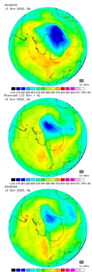
Figure 4 shows the 4-day forecast that was produced on 15 November, together with the analysis fields for 15 and 19 November. The initial field (first panel) shows the ozone hole displaced in the direction of Southern Africa. By this time the ozone layer has already recovered significantly and the area of the depleted region is a factor of 3 smaller than in early September. The forecast run performed on this day (second panel) predicts a breakup of the hole. Almost half of the depleted air is predicted to mix with mid-latitude air, re-sulting in a significant lowering of midlatitude ozone below Southern Africa. A small part of the depleted air is predicted to move in the direction of New Zealand as a narrow fila-ment. The last panel in Fig. 4 shows that this prediction ver-ifies well with the analysis on 19 November. The two ozone maps show a slightly different partitioning of the air masses, a quantity which is quite sensitive to details in the forecast wind fields.

4.2 Low ozone episode over northern Europe

Low ozone events (ozone mini-holes) over Europe have at-tracted considerable attention recently (see, for instance, Bo-jkov and Balis, 2001; Allen and Nakamura, 2002). Ozone miniholes often occur over the Atlantic and Northern Europe.

Fig. 4. The final days of the 2000 ozone hole. Top: Southern

Hemi-sphere ozone on 15 November 2000. Centre: four day forecast for 19 November. Bottom: Verification on 19 November.

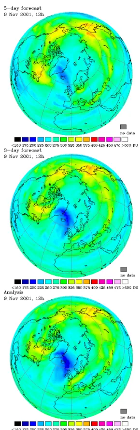
Fig. 5. The first large ozone hole of the winter 2001–2002, on 9

November 2001. Top: 5-day forecast. Centre: 3-day forecast. Bot-tom: Verification.

The lowest ozone values last only for about 1–2 days, and these events are mainly of dynamical origin, with transport of air with low ozone mixing ratios from the subtropics to higher latitudes.

In Autumn/Winter 2001/2002 a series of such low ozone events occurred. Figure 5 shows a forecast of the first large low ozone event of this winter. The five-day forecast (first panel) predicts a thin ozone layer above Iceland and the Atlantic, in qualitative agreement with the analysis and the GOME data 5 days later. Also the ozone patterns agree well with the verifying analysis (third panel). The three day fore-cast (second panel) predicts even lower values at essentially the same location, and this forecast is very close to the obser-vations on 9 November with minimum ozone values below 200 DU.

5 Conclusions

To summarise, an ozone data assimilation and forecast sys-tem has been presented. The syssys-tem is based on a transport-chemistry model driven by ECMWF meteorological fore-casts, and assimilates near-real time total column ozone mea-surements of the GOME spectrometer. The produced ozone analysis is realistic, and the detailed ozone distribution com-pares favourably with independent ozone observations from TOMS. The short-range forecast that is part of the analysis show a small bias (generally < 1%) and is able to predict the new GOME observations with a globally averaged precision of about 3%.

Based on these ozone analyses, five-day ozone forecast runs are performed routinely, and the quantitative perfor-mance of this forecast system has been presented. The re-sults, collected over the period between December 2000 and January 2002, demonstrate that medium range ozone fore-casts can be performed with a quality similar to geopotential height anomaly forecasts. The (modified) anomaly correla-tion in the extratropics crosses the value of 0.6 after about 6 days with the present setup, and therefore meaningful ozone forecasts can be produced for a period of almost one week. In the tropics the anomaly statistics are significantly worse, and we attribute this to a combination of the size of the anomaly in the tropics (r.m.s. only 2–3%), noise in the GOME ob-servation and retrieval code, and the absence of tropospheric chemistry in our model. It was shown that extreme events such as ozone mini-holes and the South Pole ozone hole can be forecast successfully 4–5 days in advance.

Ozone forecasts have a wide range of applications, includ-ing:

– UV forecasts and UV warnings (e.g. in case of

excur-sions of the ozone hole over South America)

– Prediction of special events, e.g. breakup ozone hole,

278 H. J. Eskes et al.: Global ozone forecasting

– Planning of measurement campaigns, validation

activi-ties.

An extension of the ozone forecasts with forecast of the global (clear-sky) UV index has recently been implemented, and is discussed in Allaart et al. (2002).

Numerical weather prediction centres, such as NOAA-NCEP and ECMWF, have started activities to assimilate ozone data from operational and research satellite instru-ments. In the coming years we can expect ozone forecast products of similar or better quality than the system de-scribed here. A natural future extension of these activities is forecasting of the stratospheric and tropospheric chemical composition (chemical weather). This may be achieved by coupling more extensive chemistry schemes to NWP models, in combination with the assimilation of new observations of the chemical composition of the atmosphere as provided by satellite missions such as ENVISAT and EOS-AURA.

Acknowledgements. We thank Robert Mureau for stimulation dis-cussions. This work was supported by the European Union (GOA project, contract no. EVK2-CT-2000-00062) and the Netherlands Remote Sensing Board (BCRS).

References

Allaart, M., van Weele, M., Fortuin, P., and Kelder, H.: An im-proved UV-index as function of solar zenith angle and total ozone, preprint, 2002.

Allen, D. R. and Nakamura, N.: Dynamical reconstruction of the record low column ozone over Europe on 30 November 1999, Geophys. Res. Lett., 29, cit:1362, doi:10.1029/2002GL014935, 2002.

Bojkov, R. D. and Balis, D. S.: Characterisation of episodes with ex-tremely low ozone values in the northern middle latitudes 1957– 2000, Ann. Geophysicae, 19, 797–807, 2001.

Burrows, J. P., Weber, M., Buchwitz, M., Rozanov, V., Ladst¨atter-Weibenmayer, A., Richter, A., Debeek, R., Hoogen, R., Bram-stedt, K., Eichmann, K.-U., Eisinger, M., and Perner, D.: The Global Ozone Monitoring Experiment (GOME): Mission con-cept and first results, J. Atmos. Sciences, 56, 2, 151–175, 1999. Cariolle, D. and D´equ´e, M.: Southern Hemisphere medium-scale

waves and total ozone disturbances in a spectral generated circu-lation model, J. Geophys. Res., 91, 10 825–10 846, 1986. D´equ´e, M.: Ensemble size for numerical seasonal forecasts, Tellus,

49A, 74–86, 1997.

Eskes, H. J., van Velthoven, P. F. J., Valks, P. J. M. and Kelder, H. M.: Assimilation of GOME total ozone satellite ob-servations in a three-dimensional tracer transport model, Q. J. R. Meteorol. Soc., 2002 (in press) .

Fisher, M. and Lary, D. J.: Lagrangian four-dimensional variational data assimilation of chemical species, Q. J. R. Meteorol. Soc., 121, 1681, 1995.

Fishman, J., Watson, C. E., Larsen, J. C., and Logan, J. A.:

Dis-tribution of tropospheric ozone determined from satellite data, J. Geophys. Res., 95, 359–361, 1990.

Flatøy, F., Hov, Ø., and Schlager, H.: Chemical forecasts used for measurement flight planning during POLINAT 2, Geophys. Res. Lett., 27, 951–954, 2000.

Jeuken, A. B. M., Eskes, H. J., van Velthoven, P. F. J., Kelder, H. M., and Holm, E. V.: Assimilation of total ozone satellite measure-ments in a three-dimensional tracer transport model, J. Geophys. Res., 104, 5551–5563, 1999.

Khattatov, B. V., Lamarque, J.-F., Lyjak, L. V., Menard, R., Lev-elt, P., Tie, X., Brasseur, G. P., and Gille, J. C.: Assimilation of satellite observations of long-lived chemical species in global chemistry transport models, J. Geophys. Res., 105, 29 135– 29 144, 2000.

Lalaurette, F. and Ferranti, L.: Verification statistics and evaluations of ECMWF forecasts in 2000–2001, ECMWF Technical Memo-randum 346, September 2001.

Lee, A. M., Carver, G. D., Chipperfield, M. P., and Pyle, J. A.: Three-dimensional chemical forecasting: a methodology, J. Geo-phys. Res., 102, 3905–3919, 1997.

McPeters, R. D., Bhartia, P. K., Krueger, A. J., Herman, J. R., Wellemeyer, C. G., Seftor, C. J., Jaross, G., Torres, O., Moy, L., Labow, G., Byerly, W., Taylor, S. L., Swissler, T., and Ce-bula, R. P.: Earth Probe Total Ozone Mapping Spectrometer (TOMS) Data Products User’s Guide, NASA Technical Publica-tion 1998-206895, NASA Goddard Space Flight Center, Green-belt, Maryland 20771, 1998.

Prather, M. J.: Numerical advection by conservation of second-order moments, J. Geophys. Res., 91, 6671–6681, 1986. Riishøjgaard, L. P.: On four-dimensional variational assimilation of

ozone data in weather-prediction models, Q. J. R. Meteorol. Soc., 122, 1545–1571, 1996.

˘Stajner, I., Riishøjgaard, L. P., and Rood, R., B.: The GEOS ozone data assimilation system: specification of error statistics, Q. J. R. Meteorol. Soc., 127, 1069–1094, 2001.

Simmons, A. J., Mureau, R., and Petroliagis, T.: Error growth and estimates of predictability from the ECMWF forecasting, Q. J. R. Meteorol. Soc., 121, 1739–1771, 1995.

Stoffelen, A., Eskes, H., and Kelder, H.: The EU SODA project, final report, KNMI, De Bilt, the Netherlands, 1999.

Struthers, H., Brugge, R., Lahoz, W. A., O’Neill, A., and Swin-bank, R.: Assimilation of Ozone Profiles and Total Column Mea-surements into a Global General Circulation Model, J. Geophys. Res., in press, 2002.

UNEP/WMO: “Scientific assessment of ozone depletion: 2002”, United Nations Environmental Programme and World Meteoro-logical Organisation, 2002.

Van der A, R. J., Eskes, H. J. van Geffen, J., van Oss, R. F., Piters, A. J. M., Valks, P. J. M. and Zehner, C.: GOME Fast delivery and value-Added Products (GOFAP), Proceedings of the ESA ERS – ENVISAT Symposium, Gothenburg, Sweden, 16–20 October 2000.

Valks, P. J. M., Piters, A. J. M., Lambert, J. C., Zehner, C., and Kelder, H.: A fast delivery system for the retrieval of near-real time ozone columns from GOME data, Int. J. Remote Sensing, in press, 2002.