Validation of GOME ozone profiles by means of the ALOMAR ozone lidar

HAL Id: hal-00317150

https://hal.archives-ouvertes.fr/hal-00317150

Submitted on 1 Jan 2003

HAL is a multi-disciplinary open access

archive for the deposit and dissemination of

sci-entific research documents, whether they are

pub-lished or not. The documents may come from

teaching and research institutions in France or

abroad, or from public or private research centers.

L’archive ouverte pluridisciplinaire HAL, est

destinée au dépôt et à la diffusion de documents

scientifiques de niveau recherche, publiés ou non,

émanant des établissements d’enseignement et de

recherche français ou étrangers, des laboratoires

publics ou privés.

Validation of GOME ozone profiles by means of the

ALOMAR ozone lidar

G. Hansen, K. Bramstedt, V. Rozanov, M. Weber, J. P. Burrows

To cite this version:

G. Hansen, K. Bramstedt, V. Rozanov, M. Weber, J. P. Burrows. Validation of GOME ozone profiles

by means of the ALOMAR ozone lidar. Annales Geophysicae, European Geosciences Union, 2003, 21

(8), pp.1879-1886. �hal-00317150�

Annales

Geophysicae

Validation of GOME ozone profiles by means of the ALOMAR

ozone lidar

G. Hansen1, K. Bramstedt2, V. Rozanov2, M. Weber2, and J. P. Burrows2

1_{Norwegian Institute for Air Research (NILU), Polar Environmental Centre, N-9296 Tromsø, Norway}

2_{Institute of Environmental Physics (IUP), University of Bremen FB1, P.O. Box 330 440, D-28334 Bremen, Germany}

Received: 18 June 2002 – Revised: 31 January 2003 – Accepted: 17 February 2003

Abstract. Ozone vertical profiles derived from nadir mea-surements of the GOME instrument on board the ERS-2 satellite, by means of the FURM algorithm of the Univer-sity of Bremen, are validated against measurements with the stratospheric ozone lidar at the ALOMAR facility in North-Norway. A set of 43 measurements, taken in the period Au-gust 1996 to September 1999 with a maximum distance be-tween the ground-based site and the GOME pixel centre of 650 km, is used. The comparison shows a satisfactory agree-ment within less than ±7% in the altitude range 15 to 30 km, independent of the season of the year. At lower altitudes, av-erage deviations of the GOME profiles from lidar measure-ments of up to −15% occur in spring, the reason for which has to be found in the FURM algorithm, while the agreement is within ±5% in both winter and summer/autumn months. At altitudes above 30 km, significant seasonally varying dis-crepancies occur, being largest in winter (−40% on average at 40 km altitude) and smallest in summer (less than −10%). The source of these deviations is most likely related to a ra-diance and irrara-diance calibration problem in the GOME data below 300 nm, which are used to derive ozone at the highest altitudes. The validation also shows that it is very important to choose the right ozone climatology for initialisation. Sat-isfactory results in spring 1997, when the polar stratospheric vortex was very stable, are only achieved, if a winter (vortex) profile is used.

Key words. Atmospheric composition and structure (mid-dle atmosphere-composition and chemistry; instruments and techniques; general or miscellaneous)

Correspondence to: G. Hansen (ghh@nilu.no)

1 Introduction

With the launch of the Global Ozone Monitoring Experiment (GOME) onboard the ERS-2 satellite in 1995, the European research community started a series of independent measure-ments of key atmospheric trace gases on a global scale (e.g. Burrows, 1991; ESA, 1995). The use of the DOAS (Differen-tial Optical Absorption Spectrometry) algorithm (e.g. Platt, 1994; Burrows et al., 1999) allowed the derivation of several constituents from the same data set but it also required a care-ful and comprehensive validation. This was done extensively with respect to the GOME standard products, i.e. ozone and nitrous oxide (NO2) total columns, both during the

commis-sioning phase in 1995/1996 and throughout the lifetime of GOME so far (e.g. ESA, 1996; Lambert et al., 1999; Hansen et al., 1999).

The derivation of ozone profiles was of a more experi-mental character; several parallel attempts have been made to derive an optimum of information on the vertical ozone distribution from the GOME nadir atmospheric backscatter spectra (van der A et al., 1998, Munro et al., 1998, Hoogen et al., 1998, 1999a, 1999b; Hasekamp and Landgraf, 2001).

In this paper, we present the results of a validation ex-ercise for the profile algorithm, as described in Hoogen et al. (1999a,b), which was termed the Full Retrieval Method (FURM). A first validation of this profile algorithm was per-formed using a large set of ozonesondes, which give reli-able results below altitudes of about 28 km (Hoogen et al., 1999a, b). In the framework of the European project GO-DIVA (GOME Data Interpretation, Validation and Appli-cation), ozone profiles derived from GOME measurements were validated by means of ozone profiles measured with the ALOMAR ozone lidar. With the lidar technique, reli-able ozone profiles are obtained from about 10 km up to al-titudes of 40 to 50 km, depending on observation conditions. These results are compared with past validation results using ozonesondes and other satellite instruments.

1880 G. Hansen et al.: Validation of GOME ozone profiles

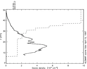
Fig. 1. Ozone profile measured with the ALOMAR ozone lidar on

9 April 1997, 21:37–23:21 UT. Uncertainties derived from the slope fit procedure (see text) are marked as horizontal bars. Dashed line: altitude range used for the slope fit, e.g. 1.5 km (5 vertical range gates) in the altitude range 7–23 km).

2 Instruments and techniques

2.1 The Global Ozone Monitoring Experiment (GOME) sensor and the FURM algorithm

The GOME sensor is a grating spectrometer aboard the ERS-2 satellite, which was launched in April 1995 (Burrows et al., 1999a). GOME covers a spectral range from 240 nm to 790 nm, with a spectral resolution of between 0.2 nm (UV) and 0.4 nm (visible). It is a nadir viewing instrument, mea-suring the radiation scattered back or reflected from the Earth and its atmosphere. The short-wave region of GOME covers the Hartley-Huggins ozone bands, which contain information about the vertical ozone distribution.

The Full Retrieval Method (FURM) algorithm utilizes this information to derive ozone profiles. FURM is an advanced Optimal Estimation inversion scheme, based on the radia-tive transfer code GOMETRAN as forward model to derive ozone profiles from the GOME UV spectra (Hoogen et al., 1999a, b). GOMETRAN was specifically designed for the evaluation of GOME data without, however, being restricted to this particular application (Rozanov et al., 1997).

FURM consists of two major parts:

– the forward model GOMETRAN, a pseudo-spherical multiple scattering radiative transfer model, calculating the top-of-atmosphere (TOA) radiance for a given state of the atmosphere;

– an iterative inversion scheme that adjusts the above state to match that calculated with the measured TOA radi-ance, utilizing the so-called weighting functions also provided by GOMETRAN.

Since the inversion is under-constrained, an optimal es-timation approach is used, combining the measurement in-formation with statistical a priori inin-formation from an ozone climatology. This retrieval uses the statistics (zonal means and standard deviations) from Fortuin and Kelder (1999) as additional constraints. The present version also contains cor-rections of the instrument calibration. Additional retrieval parameters allow the algorithm to effectively improve the calibration. A detailed description of the FURM algorithm is given by Hoogen et al. (1999b).

The ground pixel area covered by the GOME ozone profile is approximately 960 km (across-track) times 100 km (along-track). This area is larger than the footprint of GOME to-tal ozone, derived using the DOAS method (320 km times 40 km). The reason for the large ground pixel size of the GOME profiles is the fact that the integration time below 307 nm is 12 s, while it is 1.5 s for all other GOME channels (Burrows et al., 1999; Hoogen et al., 1999b). The continu-ous wavelength region of 290–345 nm was selected for the inversion.

The vertical resolution of the GOME profiles is, typi-cally, 7–8 km, estimated from the full width at half maxi-mum (FWHM) of the averaging kernels and increases above and below the region of the ozone number density maximum near 20–23 km altitude (Hoogen et al., 1999b).

2.2 The ALOMAR ozone lidar

The Norwegian ozone Differential Absorption Lidar (DIAL) system is located at the Arctic Lidar Observatory for Middle Atmosphere Research (ALOMAR) on the North-Norwegian island of Andøya (69.3 N, 16.0 E, 379 m a.s.l.). The system is of standard design, using 308 nm as the “on” wavelength (ozone extinction) and 353 nm as “off” wavelength (refer-ence atmospheric backscatter without ozone extinction). In the routine mode, backscatter profiles with a vertical resolu-tion of about 100 m and a time resoluresolu-tion of, typically, five minutes are gathered. In order to calculate ozone profiles from 10 to 45 km altitude, about one hour of measurements has to be integrated. In addition, the backscatter profiles are summed up over 3 altitude channels, respectively, which yields an altitude resolution of about 300 m at best. However, since the DIAL method is based on the ratio of the slopes of the 308- and the 353-nm signal to calculate the density at a certain altitude, the ratios of the neighbouring altitudes have also to be used. The number of points to be included in the slope fit depends upon the signal-to-noise ratio of the backscatter profiles. In the case of the ALOMAR ozone li-dar, in the lowest part of the profile, five points are used to calculate the slope; from an altitude of 25 km below the up-permost altitude and upwards the number of points is gradu-ally increased from five to 33 points at the uppermost levels. Figure 1 shows a typical ozone profile as well as the altitude filter width used in the respective altitude. This method com-plicates the comparison with the GOME profile somewhat, since the altitude resolutions are comparable in the upper part of the profile, but not in the lower part.

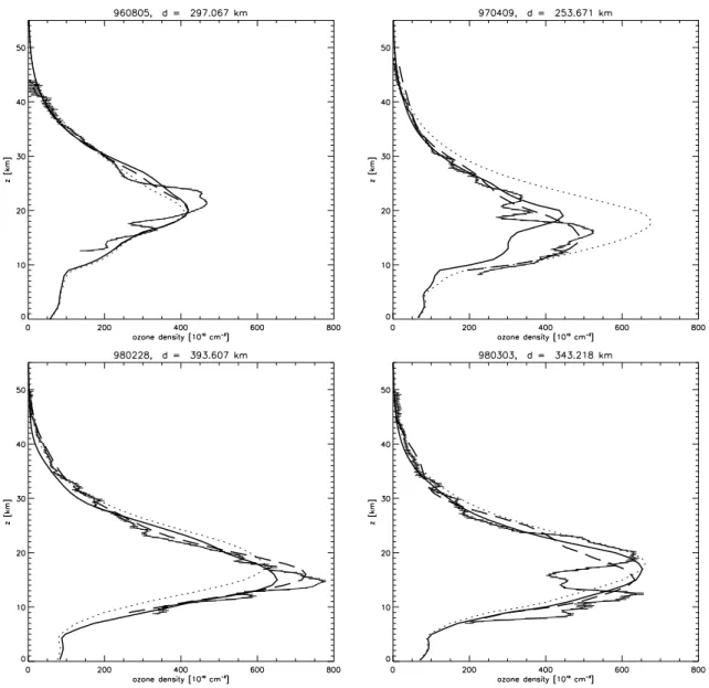
Fig. 2. Single ozone profile comparisons between ALOMAR ozone lidar and GOME: 5 August 1996 (upper left), 9 April 1997 (upper right),

28 February 1998 (lower left), 3 March 1998 (lower right). Thin solid line with error bars: full resolution lidar profile; dashed line: convolved lidar profile; bold solid line: GOME FURM profile; dotted line: a priori profile used in FURM. Value d in plot titles: distance between lidar site and GOME pixel centre.

3 Results

In total, 43 single profiles from the period August 1996– September 1999 were compared. The distance between the lidar site and the centre point of the GOME pixel is 650 km or less. Seasonally, comparisons are limited to the periods late February to early May and late July to end of September. This is caused by two limiting factors:

– Currently, GOME profiles can only be derived with the FURM algorithm at solar zenith angles less than 75◦ due to changes in integration times. At latitudes of 65 to 70◦, this excludes measurements in the period October– February.

– The lidar in its basic technical configuration can be op-erated only at solar zenith angles of more than 93◦. This

excludes measurements in the period 10 May – 30 July at the instrument site (midnight sun).

Despite this strong limitation in the exploitable time win-dows, the data set used is of great value and is also repre-sentative because the measurements included cover periods when characteristic features of the ozone layer at sub-arctic latitudes occur:

– A relatively stable layer with minimum total ozone con-tent (high tropopause level) in late summer and autumn. – A highly variable ozone layer depending on the loca-tion of the site relative to the stratospheric polar vortex in late winter/spring. The used winter/spring profiles cover conditions with the site being outside and inside

1882 G. Hansen et al.: Validation of GOME ozone profiles

Fig. 3. Relative deviation [%] between GOME and convolved lidar profiles ({GOME-lidar}/lidar) of all profiles within a 650 km radius around

ALOMAR (left panel) and within a 300 km radius (right panel). Solid bold line: average deviation; thin solid lines: standard deviations; dots: single profile deviations. Dashed line: average deviation using original (unconvolved) lidar profiles.

the polar stratospheric vortex; this has a profound im-pact on the ozone profile shape .

As already pointed out above, GOME and lidar mea-surements require contrary illumination conditions; GOME needs daylight, while the lidar requires darkness. This neces-sarily leads to a temporal offset of up to 12 h between ozone profiles to be compared. However, except in extreme situ-ations during vortex-edge episodes, the temporal variability of the ozone layer is very limited and hardly noticeable after the convolution of the lidar profile with the GOME averaging kernel functions.

Figure 2 shows four examples of single-profile compar-isons. The thin solid lines with horizontal bars represent the lidar measurement (with its measurement uncertainty), while the bold solid line is the derived GOME profile. The dotted line shows the a priori (climatological) ozone profile used in the GOME algorithm. As already pointed out, the true verti-cal resolution of the two data sets is very different. In order to allow a more realistic comparison, the lidar profiles were convolved with the average kernel functions from the GOME profile retrieval; the resulting profiles are shown as dashed lines in Fig. 2. As expected, this operation removes more or less all structures with vertical scales less than 5 km. A prominent example is the profile from 3 March 1998, with a strongly depleted layer from 13 to 18 km (lower right panel). This feature vanishes completely in the convolved lidar pro-file.

Figure 3, left panel, gives the relative deviations of the GOME profile from the convolved lidar profile of all 43 cases included in this analysis. The single-profile deviations are marked with dots, while the bold solid line gives the average deviation and the thin solid lines the standard deviation of the single relative deviations. The average deviations are less

than 10% from about 9 to 34 km; from 18 to 30 km they are even less than about 2%. Below 15 km, the average devia-tion remains practically constant at −6%, while it increases monotonously above 30 km and reaches a maximum of about

−25% at 44 km altitude. The standard deviation is also fairly constant (around 8%) in the 18-to-30 km range. It increases to about double that value at lower altitudes while it increases continuously above 30 km to reach a maximum of about 20% at altitudes above 40 km.

Using the original instead of the convolved lidar profiles does not change the results substantially. The average devi-ation profile based on the original lidar profiles is depicted as a dashed line in Fig. 3; it lies within ±5% of the aver-age ratio based on convolved lidar profiles between 15 and 40 km. The discrepancy only increases at the uppermost al-titudes, where the uncertainties of the lidar profiles become very large while, at the lowermost levels, there is a slight offset towards the zero deviation line.

The choice of a more restrictive maximum distance be-tween the ground station and the GOME pixel centre does not have a strong impact on the comparison result, as the right panel of Fig. 3 demonstrates. There, only cases with a distance less than 300 km are included, a total of 24 out of the 43 cases. Both the average discrepancies and the stan-dard deviation values of the discrepancies are practically the same as for the 650-km distance criterion. This is, at least partially, due to the fact that the across-orbit extension of the ground pixel of the GOME observations is larger than the distance criterion chosen. An even more restrictive maxi-mum distance was not investigated because of the resulting small number of remaining cases.

As illumination conditions and a priori information from a climatology are important parameters in the analysis al-gorithm, seasonal sub-sets of the data were investigated

Fig. 4. As Fig. 3, with 650 km radius, but only for the months of

August and September.

separately. This analysis revealed a pronounced difference in the deviations at higher altitudes. Figure 4 shows the rela-tive deviations for the 15 cases of the summer/autumn period. The average deviation between the GOME and the lidar pro-files is obviously much better than for the entire data set; it remains within the ±10% range throughout the whole alti-tude range covered, i.e. from 10 to 45 km. The average rela-tive deviation based on the original lidar profiles, on the other hand, oscillates much stronger around the deviation based on the convolved profiles. This is probably due to the very lim-ited number of profiles included. The good agreement over the whole altitude range is particularly surprising, because the lidar measurement accuracy in late summer/early fall is lower than in winter due to the adverse background illumina-tion condiillumina-tions.

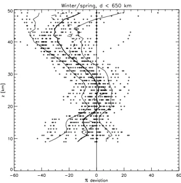
The results of an equivalent analysis for the winter/spring period is shown in Fig. 5. The deviations in this season are significantly larger than for the summer/autumn cases over most of the altitude range, especially below 15 and above 30 km altitude, where values of −10% and +30%, respec-tively, are reached. The altitude dependence of the relative deviations is similar to the all-season case. The standard deviation of the relative deviations is comparable to that of the summer data comparison. The single profile deviations (dots) indicate that the larger deviations below 15 km altitude are mainly caused by few profiles with very large deviations, while most profiles remain in the ±10% range. A survey of the single profiles showed that these cases are characterised by significant ozone deficiencies (low-ozone laminae) in the GOME profiles, while such laminae are almost completely removed from the lidar profiles after convolution with the GOME average kernel functions. All of these occur during

Fig. 5. As Fig. 3, with 650 km radius, but only for winter/spring

(end of February to early May).

the late phase of the polar vortex (April and May 1997 and 1998).

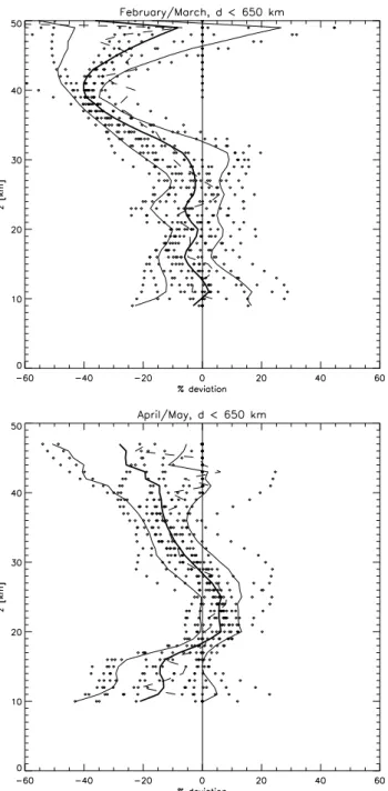
A further splitting of the winter/spring data set shows that the deviations for February/March (upper panel) and April/May (lower panel) differ widely (Fig. 6). In February and March the deviations are constantly small (−6%) from 10 to 30 km, but increase rapidly at higher altitudes, reach-ing a maximum of −40% at 40 km altitude. In April and May, the large negative deviation at high altitudes observed in the preceding months reduces to about half of that value, although the relative deviations increase to +8% in the 20-to-30 km altitude range and up to −20% below 20 km.

4 Discussion

The above results allow us to divide the altitude range cov-ered by both methods (9–45 km) into three regimes. Below 17 km, GOME on average underestimates the lidar measure-ments and the standard deviation of the relative differences is larger than in the altitude range above. At the lowest al-titudes, this is not surprising, as they cover the tropopause region where large vertical gradients and also significant hor-izontal gradients can occur. Large vertical gradients on vary-ing altitudes (because of changvary-ing tropopause heights) are smeared out in a climatology. In addition, the inversion re-sults in a smoothed difference profile with respect to the ref-erence a priori profile. Therefore, GOME can not repro-duce rapid changes in the vertical gradient causing a sys-tematic bias even in the mean difference. Comparisons be-tween the ALOMAR lidar and ozonesonde profiles from So-dankyl¨a (about 400 km SE of Andøya), launched almost si-multaneously, have at times revealed large differences in the

1884 G. Hansen et al.: Validation of GOME ozone profiles

Fig. 6. As Fig. 3 with 650 km radius, but only for the months of

February/March (upper panel) and April/May (lower panel).

tropopause altitude with a severe impact on the ozone con-centration in upper troposphere/lower stratosphere (UTLS) region (Hansen and Kyr¨o, private communication, 2002).

The best agreement is found in the medium altitude regime extending from about 17 to 30 km, with average relative de-viations of −5 to +8%, depending on the season. This is the region from slightly below the ozone maximum to about the upper half maximum of the ozone layer. Except in years of strong ozone depletion, this region in the ozone layer shows moderate or little short-time variability. The largest change with altitude of the deviations is found in the transi-tion months April and May. This could be a consequence of

the break-up of the polar stratospheric vortex at this time of the year with filaments and fragments of the vortex passing frequently over a station like ALOMAR. Such structures can cause a marked vertical variation of the ozone layer max-imum over ranges less than the distance between ground-based and GOME measurement or times scales less than the mismatch between GOME and the lidar.

In fact, an extreme event of this type is covered by this study: In 1997, the polar vortex existed until early May which, compared to other recent cold winters, such as 1995/96 and 1999/2000, corresponded to a delay of vor-tex break-up by about a month (Coy et al., 1997; Hansen and Chipperfield, 1999; Weber et al., 2002). Therefore, the monthly ozone climatology used in FURM is not represen-tative for April 1997. One should also keep in mind that the Fortuin-Kelder climatology was derived from data available before 1991 (Fortuin and Kelder, 1998). In this specific case the March climatology was used as a priori information in the FURM retrieval. The current GOME ozone profile retrieval contains an effective calibration correction introducing addi-tional fit parameters. To separate properly the ozone informa-tion contained in the spectra from the calibrainforma-tion errors, the a priori information has to be carefully selected to stabilize the retrieval solution. The upper right panel of Fig. 2 shows an example from April 1997 with reasonable agreement with the collocated lidar profile.

The deviations in the two lower altitude regimes dis-cussed so far can be compared with results of Hoogen et al. (1999), who validated GOME profiles with ozonesonde profiles from, among others, Sodankyl¨a, Finland, which is almost at the same latitude as Andøya. The Sodankyl data set covers a period of one year, but consists of only 19 single comparisons. As at Andøya, the illumination conditions ex-clude GOME profiles in late autumn and winter, while they may contain midsummer comparisons. Although the devia-tions found by Hoogen et al. are within a standard deviation of the present study, the vertical variation of the deviations is quite different. Firstly, they are generally shifted towards positive deviations and, secondly, they reveal two deviation maxima, at 12 and 25 km altitude, which are much less pro-nounced in the lidar GOME comparison. One should also note that there are substantial differences between the aver-age deviation profiles from the various ozonesonde stations, especially in the 20-to-30-km altitude range which are not explained by Hoogen et al. (1999).

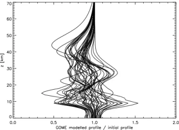
In the uppermost altitude regime (above 30 km), which is not covered by the ozonesonde analysis of Hoogen et al., there is a marked change in the deviations from win-ter to summer/autumn, being (negatively) largest in winwin-ter, reduced in spring and smallest during summer. This indi-cates that the problem is linked to solar elevation or illumi-nation conditions. Although a contribution of the increased uncertainty of the lidar profiles at the uppermost levels can-not be ruled out, the problem is most probably inherent to the GOME data. Figure 7 shows the ratios between the a priori and the fitted GOME profiles for the whole data set. With three exceptions, all a priori profiles were changed by

Fig. 7. Profiles of the ratio between the GOME profile calculated

with FURM and the respective a priori profile used in the calcula-tion for all cases analysed.

FURM towards smaller values above 33 km with a maximum change of up to −50% at about 40 km. At other altitudes, the modification is mainly negative but here numerous positive modifications of the same size also occur. The reason for this behaviour is most probably found in calibration prob-lems in the wavelength region below 300 nm of the GOME sensor. As the intensity of the signal is decreasing rapidly below 300 nm, the signal-to-noise ratio is much worse. In addition, the degradation of the instrument increases with shorter wavelength. Because the degradation depends on the scan mirror position, the use of sun-normalised radiation cannot completely cancel the effect. Below 290 nm, NOγ -Bands occur, which cannot be described by the used GOME-TRAN version and, therefore, are not used in the present version of the algorithm. The shorter wavelength gives in-formation about the higher levels of the atmosphere; using wavelengths above 290 nm limits the reliable altitude range to about 35 km.

These findings, at altitudes above 30 km, can be compared with the results of a validation study with HALOE measure-ments by Bramstedt et al. (2002). In the 60◦-to-80◦N lat-itude band, during the summer months this study revealed deviations shifted towards positive values compared to this study with a maximum of about +18% at 25 km and more than 15% all the way up to 40 km while it approaches the results presented here at lower altitudes. In winter/spring, the deviations and the large deviation gradient above 25 km altitude is quite similar to our findings, confirming the hy-pothesis that the reason is to be found in the GOME data set. At lower altitudes, GOME values are larger than HALOE values, which implies that the HALOE data underestimate ground-based high-resolution data. This is in agreement with results from other validation studies including ground-based measurements and satellite limb measurements (e.g. Hansen et al., 1998). Here, one can in fact expect that nadir mea-surements, such as those from GOME, are closer to high-resolution point measurements than limb measurements.

5 Conclusions and outlook

Although this validation study is based on a very limited data set (43 profiles), it allows some important conclusions on the quality of GOME vertical ozone profiles. The com-parison with lidar measurements at a sub-Arctic station re-vealed a satisfactory agreement in the 15-to-30 km altitude range. This is important with respect to the quantification of stratospheric ozone loss, which occurs almost completely in this altitude range (Eichmann et al., 1999, 2002; Weber et al. 2000). At lower altitudes, the agreement is less good, mainly due to the increased natural variability of the ozone layer there combined with the horizontal resolution of the GOME instrument. It is, therefore, doubtful whether this situation can be improved. At high altitudes (>30 km), the GOME data set reveals significant seasonally varying de-viations from the ground-based measurements. These are probably due to a problem with (level-1) UV irradiance data from GOME, which has prevented the use of short wave-lengths below 290 nm containing most information on ozone at higher altitudes. Work on this problem is underway, aim-ing at improvaim-ing the straylight and dark current characterisa-tions. A successful completion of these efforts will improve the radiometric calibration below 300 nm and eventually per-mit the use of wavelengths below 290 nm in the profile re-trieval.

Acknowledgements. This study was partially funded by the Euro-pean Commission through the project GODIVA (project no. ENV4-CT97-0418) and by the European and the Norwegian Space Agency through the PRODEX project “Norwegian GOME Validation”. The ALOMAR ozone lidar is owned and run in common by the Nor-wegian Defence Research Establishment, the NorNor-wegian Institute for Air Research and the Andøya Rocket Range (ARR). We thank Per-Egil Nilsen, Reidar Lyngra (both ARR), and Ulf-Peter Hoppe (FFI) for their contributions to gathering the ozone lidar data. The provision of ECMWF data and ozonesonde data from Sodankyl by FMI for the lidar data analysis is also gratefully acknowledged.

Topical Editor D. Murtagh thanks a referee for his help in eval-uating this paper.

References

Bramstedt, K., Eichmann, K.-U., Weber, M., Rozanov, V., and Burrows, J. P.: GOME ozone profiles: a global validation with HALOE measurements, Adv. Space Res., accepted, 2002. Burrows, J. P., Schneider, W., and Chance, K. V.: GOME and

SCIA-MACHY: Remote sensing of stratospheric and tropospheric gases, Eur. Comm. Air Poll. Rep., 34, 99–102, 1991.

Burrows, J. P., Weber, M., Buchwitz, M., Rozanov, V. V., Ladst¨atter-Weißenmayer, A., Richter, A., DeBeek, R., Hoogen, R., Bramstedt, K., and Eichmann, K.-U.: The Global Ozone Monitoring Experiment (GOME): Mission Concept and First Scientific Results, J. Atmos. Sci., 56, 151–175, 1999.

Coy, L., Nash, E. R., and Newman, P. A.: Meteorology of the polar vortex: Spring 1997, Geophys. Res. Lett., 24, 2693–2696, 1997. Eichmann, K.-U., Bramstedt, K., Weber, M., Rozanov, V. V., Hoogen, R., and Burrows, J. P.: O3 profiles from GOME

satel-1886 G. Hansen et al.: Validation of GOME ozone profiles

lite data - II: Observations in the Arctic spring 1997 and 1998, Physics and Chemistry of the Earth 24, 453–457, 1999. Eichmann, K.-U., Weber, M., Bramstedt, K., and Burrows, J. P.:

Ozone depletion in the NH winter/spring 1999/2000 as measured by GOME on ERS-2, J. Geophys. Res., accepted, 2002. European Space Agency (ESA): GOME Users’ Manual, ESA

SP-1182, European Space Agency, Noordwijk, 1995.

European Space Agency (ESA): GOME Geophysical validation campaign: Final results workshop proceedings, ESA WPP-108, European Space Agency, Noordwijk, 1996.

Fortuin, J. P. F. and Kelder, H.: An ozone climatology based on ozonesonde and satellite measurements, J. Geophys. Res., 103, 31 709–31 734, 1998.

Hansen, G., Shettle, E. P., and Hoppe, U.-P.: Intercomparison of ozone profiles as measured by POAM-II and lidar, Proc. 24th Ann. Europ. Meet. on Atmos. Stud. Opt. Meth., 162–167, 1998. Hansen, G., Dahlback, A., Tønnessen, F., and Svenøe, T.: Valida-tion of GOME total ozone by means of the Norwegian ozone monitoring network, Ann. Geophysicae, 17, 430–436, 1999. Hansen, G. and Chipperfield, M. P.: Ozone depletion at the edge of

the Arctic polar vortex 1996/ 1997, J. Geophys. Res., 104 (D1), 1837–1845, 1999.

Hasekamp, O. P. and Landgraf, J.: Ozone profile retrieval from backscattered ultraviolet radiances: The inverse problem solved by regularization, J. Geophys. Res., 106, 8 077–8 089, 2001. Hoogen, R., Rozanov, V. V., Bramstedt, K., Eichmann, K.-U.,

We-ber, M., and Burrows, J. P.: Validation of ozone profiles from GOME satellite data, in: Satellite Remote Sensing of Clouds and the Atmosphere III, (Ed) Russel, J. E., Proceedings of SPIE, Vol. 3495, 367–378, 1998.

Hoogen, R., Rozanov, V. V., Bramstedt, K., Eichmann, K.-U., We-ber, M., and Burrows, J. P.: Ozone profiles from GOME satel-lite data-I: Comparison with ozonesonde measurements, Phys. Chem. Earth, 24, 447–452, 1999.

Hoogen, R., Rozanov, V. V., and Burrows, J. P.: Ozone profiles

from GOME satellite data: Algorithm description and first vali-dation, J. Geophys. Res., 104, 8263–8280, 1999.

Lambert, J.-C., van Roozendael, M., de Mazi`ere, M., Simon, P. C., Pommereau, J.-P., Goutail, F., Sarcissian, A., and Gleason, J. F.: Investigation of pole-to-pole performances of spaceborne atmo-spheric chemistry sensors with the NDSC, J. Atmos. Sci., 56, 176–193, 1999.

Munro, R., Siddans, R., Reburn, W. J., and Kerridge, B. J.: Direct measurement of tropospheric ozone distributions from space, Nature, 392, 168–171, 1998.

Platt, U.: Differential optical absorption spectroscopy (DOAS), Air Monitoring by Spectroscopic Techniques, (Ed.) Siegrist, M., Chemical Analysis Series Vol. 127, John Wiley and Sons, 27–84, 1994.

Rozanov, V. V., Diebel, D., Spurr, R. J. D., and Burrows, J. P.: GOMETRAN: A radiative transfer model for the satellite project GOME, the plane-parallel version, J. Geophys. Res., 102, 16 683–16 695, 1997.

Van der A, R., van Oss, R. F., and Kelder, H.: Ozone profile retrieval from GOME data, in Satellite Remote Sensing of Clouds and the Atmosphere III, (Ed) Russel, J. E., Proceedings of SPIE Vol. 3495, 221–229, 1998.

Weber, M., Eichmann, K.-U., Bramstedt, K., Burrows, J. P., Lee, A., and Sinnhuber, B.-M.: Vertical ozone distribution in the northern hemisphere in late winter/early spring between 1996/97 and 1999/2000: GOME satellite observation of Arctic chemi-cal ozone loss in the lower stratosphere and comparison with the 3D chemical transport model SLIMCAT, Proc. Quadrennial Ozone Symp., Sapporo, 3–8 July 2000, p. 105–106, published by NASDA, Tokyo, Japan 2000.

Weber, M., Eichmann, K.-U., Wittrock, F., Bramstedt, K., Hild, L., Richter, A., Burrows, J. P., and M¨uller, R.: The cold Arctic win-ter 1995/96 as observed by the Global Ozone Monitoring Ex-periment GOME and HALOE: tropospheric wave activity and chemical ozone loss, Q. J. Meteor. Soc., accepted, 2002.