Comparison of total ozone from the satellite instruments GOME and TOMS with measurements from the Dobson network 1996?2000

(1)

HAL Id: hal-00300883

https://hal.archives-ouvertes.fr/hal-00300883

Submitted on 2 Aug 2002

HAL is a multi-disciplinary open access

archive for the deposit and dissemination of sci-entific research documents, whether they are pub-lished or not. The documents may come from teaching and research institutions in France or abroad, or from public or private research centers.

L’archive ouverte pluridisciplinaire HAL, est destinée au dépôt et à la diffusion de documents scientifiques de niveau recherche, publiés ou non, émanant des établissements d’enseignement et de recherche français ou étrangers, des laboratoires publics ou privés.

Comparison of total ozone from the satellite instruments

GOME and TOMS with measurements from the Dobson

network 1996?2000

K. Bramstedt, J. Gleason, D. Loyola, W. Thomas, A. Bracher, M. Weber, J.

P. Burrows

To cite this version:

K. Bramstedt, J. Gleason, D. Loyola, W. Thomas, A. Bracher, et al.. Comparison of total ozone from the satellite instruments GOME and TOMS with measurements from the Dobson network 1996?2000. Atmospheric Chemistry and Physics Discussions, European Geosciences Union, 2002, 2 (4), pp.1131-1157. �hal-00300883�

(2)

ACPD

2, 1131–1157, 2002

Comparison of GOME and TOMS with the

Dobson network K. Bramstedt et al. Title Page Abstract Introduction Conclusions References Tables Figures J I J I Back Close

Full Screen / Esc

Print Version Interactive Discussion

c

EGS 2002 Atmos. Chem. Phys. Discuss., 2, 1131–1157, 2002

www.atmos-chem-phys.org/acpd/2/1131/ c

European Geophysical Society 2002

Atmospheric Chemistry and Physics Discussions

Comparison of total ozone from the

satellite instruments GOME and TOMS

with measurements from the Dobson

network 1996–2000

K. Bramstedt1, J. Gleason2, D. Loyola3, W. Thomas3, A. Bracher1, M. Weber1, and J. P. Burrows1

1

Institute of Environmental Physics, University of Bremen, Bremen, Germany

2

NASA/Goddard Space Flight Center, Greenbelt, MD 20771, USA

3

DLR Remote Sensing Technology Institute (DLR/IMF), Wessling, Germany Received: 19 June 2002 – Accepted: 17 July 2002 – Published: 2 August 2002 Correspondence to: K. Bramstedt (klaus.bramstedt@iup.physik.uni-bremen.de)

(3)

ACPD

2, 1131–1157, 2002

Full Screen / Esc

c

EGS 2002

Abstract

Over the last 3 decades, satellite data have been used to monitor long-term global changes in stratospheric ozone. The TOMS series (1978 – present) and GOME (1995 – present) are two very important instruments in this context. In this paper, TOMS total ozone and three approaches to derive total ozone from GOME measurements

5

are validated with ground-based Dobson network data. Beyond the operational prod-ucts of both instruments, e.g. TOMS Version 7 and GOME Data Processor Version 2.7, total ozone is calculated by integrating FURM ozone profiles and by applying the TOMS algorithm to the GOME spectra. All algorithms show in general good agree-ment with ground-based measureagree-ments. The operational GOME total ozone shows

10

seasonal variations, most likely introduced by difficulties in the derivation of airmass factors, which convert measured slant columns into vertical columns. The TOMS al-gorithm estimates on average 2% higher total ozone in the southern hemisphere than in the northern for both instruments as compared to the ground-based data, indicating that the source of the observed hemispheric differences is in the TOMS algorithm. Both

15

instruments show aging effects in 2000, leading to enhanced variability in the ozone column differences with respect to Dobson data. In addition, the integrated GOME ozone profiles and the TOMS algorithm applied to GOME data show larger mean devi-ations in 2000.

1. Introduction 20

The stratospheric ozone layer protects the biosphere from harmful ultraviolet radia-tion. Dramatic changes in the ozone layer during the Antarctic spring first detected byFarman et al.(1985) established the need for global measurement of atmospheric trace gases with ozone as the most important one. Longterm observation are urgently needed to assess current and future changes.

25

(4)

ACPD

2, 1131–1157, 2002

Full Screen / Esc

c

EGS 2002 location. Satellite instruments are the most effective way to achieve a global view of the

atmosphere, but have to be validated during the complete lifetime to ensure the ongoing quality of the measured data and to avoid longterm drifts in their data by instrumental aging effects.

The Total Ozone Mapping Spectrometers TOMS have been a successful series of

5

instruments designed for measuring total ozone. TOMS measures total ozone, an aerosol index, and SO₂. The Global Ozone Monitoring Experiment (GOME) is a com-bined prism and grating spectrometer. Operational data products are total columns of ozone and NO₂. Retrieval of ozone profiles and of additional trace gases have been demonstrated: BrO, SO₂, OClO, HCHO and water vapour (Burrows et al.,1999).

10

The objective of this paper is to define the drift of total ozone determined from EP-TOMS and GOME in comparison to ground-based measurements from Dobson and Brewer stations collected by WOUDC. Four datasets of total ozone are used: From TOMS, the operational Version 7 product is used. From GOME, three types of datasets are compiled: First, total ozone is calculated with the DOAS approach, which is the

op-15

erational GOME data product GDP Version 2.7. Second, total ozone is calculated by integrating GOME ozone profiles calculated with the inversion scheme FURM. Third, the TOMS algorithm is applied to the GOME spectra. Comparing different algorithms is a good way to separate the effects of instrument degradation from possible short-comings of the individual algorithms.

20

2. The instruments

Measurements from the satellite instruments GOME and TOMS are used. Both ob-serve Earth’s atmosphere in nadir geometry from a polar, sun-synchronous orbit. The ground-based network consists of Dobson and Brewer instruments.

(5)

ACPD

2, 1131–1157, 2002

Full Screen / Esc

c

EGS 2002 2.1. GOME

The Global Ozone Monitoring Experiment GOME aboard the European Remote Sens-ing Satellites ERS-2 of the European Space Agency ESA measures the backscattered and reflected solar radiation from the atmosphere and surface of the Earth in the spec-tral range from 240–790 nm with a moderate resolution of 0.2–0.4 nm. GOME

ob-5

serves the earth in nadir viewing geometry, scanning across-track ±30◦corresponding to 960 km on ground. Global coverage is reached within 3 days at the equator and faster at higher latitudes. The detectors are four Reticon SiO diode arrays with 1024 pixels for each, corresponding to 4 channels (SP–1182). Channel 1 and 2 are divided in two bands, leading to a total of six bands. Table1 lists the properties of the bands.

10

To shorter wavelength, the intensity of incoming light is drastically reduced due to the increasing ozone absorption in the Huggins-Band. Therefore, Band 1A has a longer integration time of 12 s instead of 1.5 s. After July 1998, the boundary between Band 1A and 1B has been moved from 307 nm to 283 nm. Before March 1996, the integra-tion time for the long wavelength channels were limited to 0.375 s to avoid saturaintegra-tion

15

effects, afterwards a co-adding software patch to achieve the nominal 1.5 s integration time without saturation was successfully up-linked to the satellite.

Once a day GOME solar irradiance measurements are performed, which is needed to normalise the backscattered radiances. The solar radiation enters the instrument through the sun viewport, reduced by a diffuser plate and a 20% transmission mesh

20

and directed by the sun view mirror to the scan mirror in an appropriate position. Three additional fast broadband detectors are used to determine the polarisation state of the incoming light, which is needed to take into account the polarisation sensitivity of the optical components of the instrument.

2.2. EP-TOMS

25

The Total Ozone Mapping Spectrometers TOMS have been a successful series of in-struments designed for measuring total ozone. The TOMS inin-struments use six discrete

(6)

ACPD

2, 1131–1157, 2002

Full Screen / Esc

c

EGS 2002 wavelength in the UV/visible part of the spectrum to derive total ozone, an aerosol

in-dex, and SO₂. TOMS aboard NIMBUS-7 started in 1978 and operated successfully 14.5 years, TOMS on Meteor 3 operated 1991 to 1994. TOMS aboard ADEOS was launched in 1996 and ceased operation in June 1997 with the failure of the ADEOS spacecraft. The last instrument of this series is TOMS aboard Earth Probe (EP-TOMS),

5

launched in July 1996.

Originally, the data obtained from EP-TOMS were intended to complement data ob-tained from ADEOS TOMS. The initial 500 km orbit led to smaller footprints with the disadvantage of loosing global coverage in one day. With the failure of the ADEOS spacecraft Earth Probe was lifted to higher orbit, so that EP-TOMS has almost global

10

coverage in one day since December 1997.

TOMS uses a single monochromator and a scanning mirror to sample the backscat-tered solar ultraviolet radiation at 35 sample points at 3-degree intervals along a line perpendicular to the orbital plane. It then quickly returns to the first position, not mak-ing measurements on the retrace. Eight seconds after the start of the previous scan,

15

another scan begins. EP-TOMS measures six discrete wavelengths between 309 and 360 nm, selected by a chopper wheel in the light path behind the monochromator grat-ing. The slit functions are triangular with a nominal 1 nm bandwidth.

The solar irradiance is measured using a diffuser plate to reflect sunlight into the instrument. Actually, three diffuser plates are installed, which are used at different

20

frequency. Comparisons of the signals of these diffusers allow the determination of degradation rates of the diffusers (McPeters et al.,1998).

2.3. Dobson and Brewer spectrophotometer

The first Dobson spectrophotometer was developed 1927 by G. M. B. Dobson (Dob-son and Harri(Dob-son,1926;Dobson et al., 1927, 1929;Dobson,1931). Since then this

25

type of instruments plays an important role in routine measurements of total ozone. The Antarctic ozone hole was first observed by a Dobson instrument (Farman et al., 1985), which was subsequently confirmed by the TOMS instrument (Stolarski et al.,

(7)

ACPD

2, 1131–1157, 2002

Full Screen / Esc

c

EGS 2002 1986). The measurement method uses the ozone absorption in the Huggins band.

The differential absorption at two wavelength pairs is measured to separate the ozone absorption from the scattering by atmospheric molecules and aerosols.

Dobson instruments need an accurate calibration, limiting historical records to an accuracy of 5–10% (Grant, 1989). Since the mid-1970s, virtually all instruments in

5

the Dobson network are regularly calibrated with the reference-standard Dobson spec-trophotometer M83 located in Mauna Loa, Hawaii (Komhyr et al.,1989). The relative uncertainty is now estimated to be 2% (Basher,1985).

Since the early 1970s an alternative instrument called the Brewer spectrophotometer was developed (Brewer,1973). It is capable to measure all wavelength nearly

simul-10

taneously and is easier to calibrate. Since 1982, a fully automated instrument version is available, allowing in principle a better performance (Kerr et al.,1984). In the follow-ing, the Dobson and Brewer network will be called Dobson network for simplicity, the majority of sites still operate Dobson instruments.

The Dobson network has been already used for validating total ozone (Lambert

15

et al.,2000). Version 7 of Nimbus 7 TOMS has been shown to agree within 1% with the Dobson network in the northern hemisphere for solar zenith angles up to about 80% (McPeters and Labow,1996). Dobson network data have been also used to ho-mogenise TOMS and GOME data for longterm trend assessment up to 1998 (Bodeker et al.,2001).

20

3. Algorithms

Four algorithm are used to derive total ozone from the satellite instruments, one is applied to TOMS data and three uses the GOME spectra. The following list gives an overview in conjunction with the abbreviations for the datasets used in this paper, afterwards a description of the algorithms is given.

25

(8)

ACPD

2, 1131–1157, 2002

Full Screen / Esc

c

EGS 2002

GOMEDOAS. Version 2.7 GOME total ozone.

GOMEFURM. Integrated GOME ozone profiles calculated with FURM 5.0. GOMETOMS. TOMS Version 7 total ozone algorithm applied to GOME data.

Whereas EPTOMS and GOMEDOAS are official products of the instruments, the GOMEFURM and GOMETOMS data were calculated for this paper.

5

3.1. EPTOMS

The TOMS Version 7 algorithm is similar to the approach used for Dobson instruments. Pairs of wavelengths with differential ozone absorption are used to determine the total ozone column. In a first step, one pair is used to determine an initial assumption of the total ozone by comparing the measured radiance differences with (pre-) calculated

10

differences from a radiation transfer code for a given geometry, climatological atmo-spheric conditions and a range of ozone columns. In a second step, the wavelength triplets are used to refine the initial value. The use of triplets instead of pairs allows a correction for effects linear with wavelength. The used triplet depends on the optical path length, e.g. the solar zenith angle.

15

Clouds are determined from the 360 nm wavelength, which is insensitive to ozone. The radiance is calculated for cloud free and fully cloud covered scene, than the cloud fraction is estimated as weight of the summed radiances, which match the measured radiance. In the radiative transfer model effect of clouds and aerosols are treated as effective Lambertian albedo. The cloud cover is together with ISCCP cloud climatology

20

information used to estimate the invisible ozone below the clouds (McPeters et al., 1998).

3.2. GOMEDOAS

The Differential Optical Absorption spectroscopy (DOAS,Platt,1994) is used to derive trace gases columns from GOME spectra. The DOAS algorithm determines an ozone

(9)

ACPD

2, 1131–1157, 2002

Full Screen / Esc

c

EGS 2002 slant column in the 325–355 nm spectral window (Burrows et al., 1999). Air mass

factors describe the enhancement of the absorption of a given trace gas due to slant paths of incident light in the atmosphere. A fast radiative transfer model calculates AMFs on-line, only considering single scattering effects. The multiple scattering is then accounted for by multiplicative correction factors that were derived from radiative

5

transfer simulations using GOMETRAN (Rozanov et al., 1997, 1998). Dividing the slant column by the AMF gives the vertical column. A correction for the missing ozone below clouds is applied by adding a ghost vertical column to the vertical column using fractional cloud cover information derived from the missing O₂A band absorption at 760 nm (Kuze and Chance,1994). Because the ozone fitting window is part of channel

10

2 of the instrument, for most of the orbit the ground-pixel size is 40 × 320 km. For this paper, the total ozone calculated by the GOME Data Processor (GDP) version 2.7 is used (Spurr,2000).

3.3. GOMEFURM

Height-resolved ozone information can be derived from the short-wave Hartley-Huggins

15

ozone bands. The Full Retrieval Method (FURM) derives ozone profiles from GOME sun normalised spectra (Hoogen et al., 1999). It consists of two parts: (i) a forward model, the pseudo-spherical multiple scattering radiative transfer model (RTM) GOME-TRAN (Rozanov et al., 1997) calculating the TOA (top of atmosphere) radiance for a given state of the atmosphere as defined by the ozone vertical distribution and other

20

trace gas distributions, the surface albedo, and the aerosol scenario among others, and (ii) an inversion scheme which matches in iterative steps the calculated TOA radi-ance to the measured GOME radiradi-ance by adjusting the model atmospheric parameters such as the vertical ozone distribution using appropriate weighting functions also pro-vided by GOMETRAN. An improved optimal estimation approach is used for this task

25

(Rodgers,2000;Hoogen et al.,1999). In this work, the spectral window from 290 nm to 345 nm is used. Since the spectral reflectivity varies with ground pixel area, channel 2 and band 1B data are co-added to match the scene reflectivity of the UV channel.

(10)

ACPD

2, 1131–1157, 2002

Full Screen / Esc

c

EGS 2002 The corresponding ground pixel is therefore enlarged to about 100 × 960 km (see

Ta-ble1). Larger integration times cannot be handled by the current version of FURM (5.0), therefore profile retrieval is limited to solar zenith angles below 76◦.

Profiles are retrieved on 71 altitude levels from ground to 71 km. The algorithm in-cludes an effective correction for calibration uncertainties of the GOME instrument.

As-5

similated meteorological data from UKMO are used for obtaining pressure and temper-ature profiles (Swinbank and O’Neill,1994). A-priori information about the ozone distri-bution was derived from the Fortuin and Kelder ozone climatology, based on ozoneson-des and SBUV/SBUV2 measurements between 1980 and 1991 (Fortuin,1996;Fortuin and Kelder,1998). Integrating the profiles determined with FURM yields the

GOME-10

FURM total ozone dataset. 3.4. GOMETOMS

The continuous spectrum of GOME also contains the discrete wavelengths used by TOMS. Therefore, the TOMS algorithm can be applied to derive total ozone from GOME spectral measurements. The GOME spectra are slit-averaged with a 1.1 nm

15

FWHM triangle to match the spectral bandpass of EP-TOMS. The smoothed GOME spectra are sampled at the six EP-TOMS wavelengths and the EP-TOMS Version 7 algorithm is applied to the GOME data. This approach gives the unique opportunity to investigate the separation of instrument calibration and ozone determination in the TOMS algorithm.

20

4. Data sets

The World Ozone and Ultraviolet Radiation Data Centre (WOUDC) is one of six recog-nised World Data Centres which are part of the Global Atmosphere Watch (GAW) program which in turn is part of the World Meteorological Organization (WMO). Mea-surements of ozone are collected since 1960, a large dataset contains meaMea-surements

(11)

ACPD

2, 1131–1157, 2002

Full Screen / Esc

c

EGS 2002 from Dobson and Brewer spectrometer around the world. These data are available

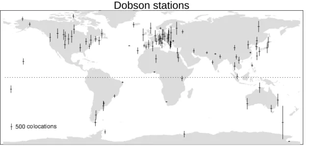
through the WOUDC website (http://www.tor.ec.gc.ca/woudc/woudc.html) (Hare and Fioletov,1998;Wardle et al.,1998). For this work, Dobson network data in the period from 1996 to 2000 are used. The stations are indicated in Fig.1.

All Dobson measurements are checked for overpasses of the two satellite

instru-5

ments at the same day. Overpass means here, that the distance between ground pixel center and Dobson station is less than 300 km. Only the nearest ground pixel is used. When a match is found, the appropriate total ozone value was calculated from the measured radiances (GOMEFURM and GOMETOMS) or collected from the official products (EPTOMS and GOMEDOAS).

10

The number of collocated data points are 52665 for GOMEFURM, 59189 for GOME-DOAS, 92332 for EPTOMS and 57052 GOMETOMS. The EPTOMS dataset is the largest one, because of the almost daily coverage of this instrument. The GOMEFURM dataset is smaller than the GOMEDOAS dataset, because some extra requirements for the GOME data are needed, the most important one is the restriction to solar zenith

15

angles below 76◦. Additionally, January to March 1996 is not used for FURM retrieval because of the missing co-adding patch for GOME.

5. Results

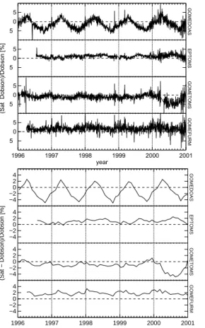
The relative differences between satellite and groundbased data were calculated. Daily and monthly (more precisely: four weekly) means of these values are produced to

ob-20

tain time series. The daily means gives an impression of the variability of the data, whereas the monthly means stress the long term variations. Figure 2 summarises the results for all four datasets, separated in northern and southern hemisphere. The datasets for the northern hemisphere are much larger than for the southern hemi-sphere, because most stations are north of the equator (see Fig.1). The results for

25

the two hemispheres are quite different. In general, the lines are less smooth in the southern hemisphere because of the reduced number of data points. The statistics are

(12)

ACPD

2, 1131–1157, 2002

Full Screen / Esc

c

EGS 2002 summarised in Table2.

GOMEDOAS total ozone is on average smaller than Dobson data by about 1.2% in the northern and 1.5% in the southern hemisphere. During the course of the year a seasonal variation from −4 to+2% in the northern hemisphere is clearly visible and is shifted by six months in the southern hemisphere. Highest positive ozone differences

5

are observed in spring and highest negative differences in autumn of each hemisphere, respectively.

The EPTOMS dataset shows a small positive bias of 1.1% in the northern hemi-sphere against the Dobson measurements, whereas in the southern hemihemi-sphere the mean offset is about 3.3%. Little seasonal variation is observed.

10

The GOMETOMS overall means are 1.2% lower in the northern and 1.1% higher in the southern hemisphere than Dobson. A similar hemispheric bias of about 2% is observed in the EPTOMS data. The seasonal variations are small in the northern hemisphere, except for 2000, where the difference decreased to −5% in summer. In general, the lowest values can be observed in summertime in the northern hemisphere,

15

but only with variations up to one half percent for the other years. In the southern hemisphere, the peaks around April and November in 1996, 1997 and 1999 can reach up to+3% and minimum values down to −4% in the second half of 2000 are noticeable. In both hemispheres, the GOMEFURM datasets give about 1.8% higher ozone val-ues. In the northern hemisphere, the variations of the mean are small to within about

20

± 1%. The highest values are usually observed in the beginning of the year with excep-tion of 1997 where the maximum moved to early March. The values decrease in the course of the year towards a minimum in the second half of the year. In the southern hemisphere, in all years local minima can be observed around May and November. In 2000, the mean difference is enlarged to about 4%.

25

The daily mean differences are smoother for the EPTOMS dataset because of the larger number of coincidences. The GOMEFURM dataset is noisier because of the lower number of matches and, most likely, because of the larger ground pixel area. Also the data from the southern hemisphere are noisier than from the northern hemisphere

(13)

ACPD

2, 1131–1157, 2002

Full Screen / Esc

c

EGS 2002 because of the smaller number of coincidences. All four datasets show an increased

variability in the daily means in 2000. The peculiar behaviour of all datasets in 2000 can be interpreted as instrumental effects in both, GOME and TOMS, as will be discussed later on.

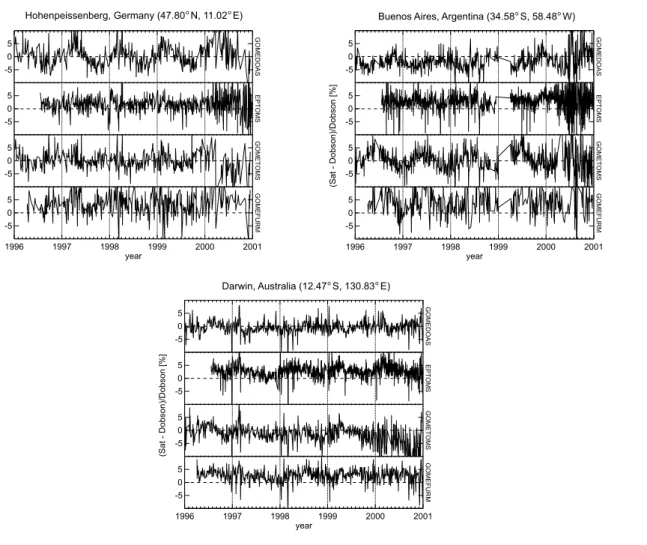
For three examples, time series at a single station are shown in Fig. 3. For the

5

northern midlatitudes, Hohenpeißenberg (Germany, 47.80◦N , 11.02◦E ) was selected, Darwin (Australia, 12.47◦S , 130.83◦E ) lies in the Tropics and Buenos Aires (Argentina, 34.58◦S , 58.48◦W ) represents southern midlatitudes. Buenos Aires has a data gap in early 1999. These plots give an impression of the variability of the individual stations, which can reach up to ± 5%. This is comparable also with the RMS of the mean relative

10

differences in Table2. In Hohenpeißenberg, the seasonal variation in the GOMEDOAS dataset is obvious, whereas it is less pronounced for Buenos Aires and Darwin. The significant decrease of the values of GOMETOMS in 2000 in the northern hemisphere is also visible in the Hohenpeißenberg dataset. The less pronounced decrease in the southern hemisphere in GOMETOMS in 2000 can be identified at the Darwin station.

15

The GOMETOMS dataset at Buenos Aires shows a seasonal variation with enhanced values in midyear and reduced values at the turn of the year.

At all stations, the increased variability of the differences in 2000 already observed in the daily means in Fig. 2 are visible. Most pronounced is this for Buenos Aires, whereas Hohenpeißenberg and Darwin appear to be less effected.

20

Figure 4 shows the mean relative difference over the entire time frame for each individual station including its standard deviation. Some stations show significantly large deviations for all datasets. Deviations of more than 5% are observed for the stations Lagos (Nigeria) with about 7%, Hanoi (Vietnam) and Mariambio (Argentina) with about 8.5% and Sofia (Bulgaria) with about −8%. 80% of the stations show mean

25

(14)

ACPD

2, 1131–1157, 2002

Full Screen / Esc

c

EGS 2002

6. Discussion

The most pronounced feature is the very regular seasonal pattern observed in the monthly mean deviations of the GOMEDOAS dataset. Similar seasonal variations were already observed for previous GDP versions in northern midlatitudes (Lambert et al., 2000). These are introduced by the airmass factor calculations. Up to the current

5

version 2.7 of the GDP, ozone climatology used for the airmass factor determination is based on a twodimensional CTM. Additionally, there are no iterations in the AMF calculations to match total ozone of the climatological ozone profiles with the observed total ozone values.

The upcoming version 3.0 of the GOME data products will introduce important

modi-10

fications to overcome this problem. The ozone climatology is replaced by the one used in the TOMS Version 7 algorithm (Wellemeyer et al., 1997). Ozone AMFs were pre-calculated using LIDORT (Spurr et al.,2001) and parameterised using neural network techniques (Loyola,1999). The total ozone content is derived using an iterative proce-dure (Spurr,1999), that searches for the best suited ozone profile. Figure 5 shows a

15

comparison of Version 3.0 with Version 2.7 for 4 April 1997. Overplotted is a line show-ing the correction proposed byBodeker et al.(2001) to homogenise total ozone GDP version 2.4 with the measurements of the Dobson network. Major changes between Version 2.4 and 2.7 were related to NO₂column retrieval, showing minor differences in total ozone. The difference between old and new GDP version generally agrees well

20

with the suggested correction, e.g. total ozone from the new GDP version are in better agreement with the DOBSON network data. Exception are measurements with solar zenith angles beyond 85◦.

The other datasets based on GOME data, GOMETOMS and GOMEFURM, show small seasonal variations. Three sources for seasonal variations are possible. First,

25

insufficient climatologies may introduce seasonal artefacts, as it is the case for GOME-DOAS. Climatological information is used in all algorithms presented here. Second, the algorithm may be sensitive to the global seasonal variations of the ozone

(15)

distribu-ACPD

2, 1131–1157, 2002

Full Screen / Esc

c

EGS 2002 tion in the atmosphere. Third, instrumental effects may introduce seasonal artefacts

to the measured spectra. For the GOME instrument, one effect of this type is known, introducing small seasonal variations to the irradiance of the instrument.

The solar intensity in GOME is reflected by a diffuser, which is a sand blasted alu-minium plate. The pattern on the surface is not perfectly random, introducing small

5

interference pattern in the diffused light which depends on the incident angle of the incoming solar light. Because of the passive tracking of the sun the incident angle of the solar beam on the diffuser has a seasonal pattern defined by the relative position of the earth-sun-satellite system.

The GOME solar spectrum is a mean of about 17 individual measurements taken in

10

sequence during full solar disc viewing (Weber et al.,1998). Therefore, these individual measurements can be used to study the effect of a changing incident angle. With the FURM algorithm, the ozone profile for one groundpixel is retrieved using the individual solar measurements for normalisation. Figure6shows the GOMEFURM total ozone from the individual solar spectra. Remarkable is the smooth variation of the ozone

15

value with the changing incident angle. Unfortunately, during these sequence of sun measurements the zenith angle at the diffuser plate varies, whereas in the course of the year the azimuthal angle varies. Therefore, a quantitative statement about the amplitude of a seasonal effect cannot be derived. Nevertheless, a small effect in the same order of 0.3% can be expected, which is too small to be clearly identified.

20

The EPTOMS dataset gives highly reproducible results with a small bias of 1.1% in the northern and a larger offset of about 3.3% in the southern hemisphere. This fea-ture of the TOMS data product was also observed by other authors (Bodeker et al., 2001;Lambert et al.,2000). Remarkable here is that the GOMETOMS dataset shows the same difference of 2.2% between the northern and southern hemisphere. This

25

difference indicates that the increased TOMS values in the southern hemisphere are most likely introduced by the algorithm and is independent of the instrument. In gen-eral, the GOMETOMS values are about 2% lower than the EPTOMS values, which are most likely due to differences in the radiometric calibration of the two instruments at the

(16)

ACPD

2, 1131–1157, 2002

Full Screen / Esc

c

EGS 2002 discrete TOMS wavelengths.

After the end of 1999, both instruments TOMS and GOME show some sign of instru-mental changes due to aging of each instrument. Both instruments are now over five years in operation.

The TOMS instrument experienced two data anomalies starting in the year 2000:

5

a drop in the throughput of the instrument and an across-track bias in the order of 3%. This error appears to be caused by changes in the optical properties of the front scan mirror (NASA,2001). This scan bias is most likely the reason for the enhanced variability in 2000.

The GOME instrument also shows degradation in the UV-part of the spectra. In

gen-10

eral, such a degradation should be cancelled out by using the sun-normalised spectra. However, recently a scan mirror angle dependent degradation was observed, which means that the solar spectra and the earthshine spectra for different scan directions degrades at slightly different rates (Snel,2001;Tanzi et al.,2001). Whereas the GOME-DOAS dataset seems to be relatively robust because of the polynomial subtraction in

15

the DOAS approach, the GOMEFURM and most noticeable the GOMETOMS are more sensitive, as seen by the drift in the satellite-Dobson differences in 2000.

7. Conclusions

The overall agreement of all satellite total ozone data sets presented here is generally very high and in most cases within the uncertainty of 2% of the Dobson

measure-20

ments. Exceptions are the enhanced EPTOMS values in the southern hemisphere, the seasonal variations of the GOMEDOAS dataset and the unusual values in 2000 in the GOMETOMS and GOMEFURM datasets.

Statistics with large datasets are a powerful tool to unveil small effects of algorithm inconsistencies and instrument effects and allow a better understanding of these

ef-25

fects. For improvement of the GOME analysis it was shown that a neural network iterative AMF algorithm and use of two ozone temperatures in the ozone crossection

(17)

ACPD

2, 1131–1157, 2002

Full Screen / Esc

c

EGS 2002 may provide longterm stability of the GOME dataset using the DOAS approach. The

future GDP version 3.0 will include these updates. The interhemispheric offset in the TOMS data are identified to be a part of the Version 7 ozone retrieval, which causes similar biases in both GOME and TOMS data. A new Version 8 TOMS algorithm is presently in preparation.

5

Aging effects of both instruments are identified in 2000 as enhanced variability in the total ozone differences. Additionally, unusual large mean differences are observed for GOMETOMS and GOMEFURM during 2000, whereas the DOAS approach apart from increasing noise appears to be stable with respect to instrument degradation.

Acknowledgements. The authors thank Gordon Labow for creating the GOMETOMS and

GOME-10

DOAS satellite/Brewer-Dobson overpass datasets. They all thank all instrument-PIs and oper-ators of the contributing instruments and the WOUDC for maintaining the groundbased mea-surement database. Financial support was given by the GOMSTRAT project as part of the na-tional German atmospheric research program (AFO2000), the BMBF project 01SF9994 (HGF-Vernetzungsfonds) and the DLR-Bonn project 50EE9909.

15

References

Basher, R. E.: Review of the dobson spectrophotometer and its accuracy, in: Atmospheric Ozone, (Eds) Zerefos, C. S. and Ghazi, A., p. 387, Reidel and Dordrect, 1985. 1136

Bodeker, G. E., Scott, J. C., Kreher, K., and McKenzie, R. L.: Global ozone trends in potential vorticity coordinates using TOMS and GOME intercompared against the dobson network:

20

1978–1998, J. Geophys. Res., 106, 23–29, 2001. 1136,1143,1144,1156

Brewer, A. W.: A replacement for the dobson spectrophotometer?, Pure Appl. Geophys., 919, 106–108, 1973. 1136

Burrows, J. P., Weber, M., Buchwitz, M., Rozanov, V. V., Ladst ¨adter-Weissenmayer, A., Richter, A., de Beek, R., Hoogen, R., Bramstedt, K., Eichmann, K.-U., Eisinger, M., and Perner,

25

D.: The Global Ozone Monitoring Experiment (GOME): Mission concept and first scientific results, J. Atmos. Sci., 56, 151–175, 1999. 1133,1138

Dobson, G. M. B.: A photoelectric spectrophotometer for measuring the amount of atmospheric ozone, Proc. Physical Society, 43, 324–338, 1931. 1135

(18)

ACPD

2, 1131–1157, 2002

Full Screen / Esc

c

EGS 2002 Dobson, G. M. B. and Harrison, D. N.: Measurements of the amount of ozone in the earth’s

atmosphere and its relation to other geophysical conditions, Proc. Royal Society London A, 110, 660–693, 1926. 1135

Dobson, G. M. B., Harrison, D. N., and Lawrence, J.: Measurements of the amount of ozone in the earth’s atmosphere and its relation to other geophysical conditions, ii, Proc. Royal

5

Society London A, 114, 521–541, 1927. 1135

Dobson, G. M. B., Harrison, D. N., and Lawrence, J.: Measurements of the amount of ozone in the earth’s atmosphere and its relation to other geophysical conditions, iii, Proc. Royal Society London A, 122, 456–486, 1929. 1135

ESA: ERS-ENVISAT Symposium, Gothenburg, 16-20 October 2000, vol. ESA SP-461,

Euro-10

pean Space Agency Publication Division, Noordwijk, on CD-ROM, 2001. 1148,1149

Farman, J. C., Peters, D., and Greisinger, K. M.: Large losses of total ozone in Antarctica reveal seasonal ClOX / NO interaction, Nature, 315, 207–210, 1985. 1132,1135

Fortuin, J. P. F.: An ozone climatology based on ozonesonde measurements, Sci. Rep. WR 96-07, KNMI, de Bilt, The Netherlands, 1996. 1139

15

Fortuin, P. and Kelder, H.: An ozone climatology based on ozonesonde and satellite measure-ments, J. Geophys. Res., 103, 31 709–31 734, 1998. 1139

Grant, W. B.: (Ed) Ozone Measuring Instruments for the Stratosphere, vol. 1 of Collected Works in Optics, Optical Society of America, Washington D. C., 1989. 1136

Hare, E. W. and Fioletov, V. E.: An examination of the total ozone data in the world ozone

20

and ultraviolet radiation data centre, in: Atmospheric Ozone - Proc. 18th Quadrennial Ozone Symposium L’Aquila, Italy, (Eds) Bojkov, R. D. and Visconti, G., pp. 45–48, PSTd’A, 1998.

1140

Hoogen, R., Rozanov, V. V., and Burrows, J. P.: Ozone profiles from GOME satellite data: Algorithm description and first validation, J. Geophys. Res., 104, 8263–8280, 1999. 1138

25

Kerr, J. B., McElroy, C. T., Wardle, D. I., Olafson, R. A., and Evans, W. F. J.: The automated brewer spectrophotometer, in: Proc. of the Quadrennial Ozone Symposium, (Eds) Zerefos, C. S. and Ghazi, A., pp. 611–614, D. Reidel Publ. Co., Dordrecht, 1984. 1136

Komhyr, W. D., Grass, R. D., and Leonhard, R. K.: Dobson spectrophotometer 83: A standard for total ozone measurements, 1962–1987, J. Geophys. Res., 94, 9847–9861, 1989. 1136

30

Kuze, A. and Chance, K. V.: Analysis of cloud top height and cloud coverage from satellites using the O2A and B bands, J. Geophys. Res., 99, 14 481–14 491, 1994. 1138

(19)

ACPD

2, 1131–1157, 2002

Full Screen / Esc

c

EGS 2002 Andersen, S. B., Arlander, D. W. ., Van, N. A. B., Claude, H., de La No ¨e, J., Mazi `ere, M. D.,

Dorokhov, V., Eriksen, P., Green, A., Trnkvist, K. K., Høiskar, B. A. K., Kyr ¨o, E., Leveau, J., Merienne, M.-F., Milinevsky, G., Roscoe, H. K., Sarkissian, A., Shanklin, J. D., Staehelin, J., Tellefsen, C. W., and Vaughan, G.: Combined characterisation of gome and toms total ozone measurements from space using ground-based observations from the ndsc, Adv.

5

Space Res., 26, 1931–1940, 2000. 1136,1143,1144

Loyola, D.: Using artificial neural networks for the calculation of air mass factors, in: Proceed-ings ESAMS’99 – European Symposium on Atmospheric Measurements from Space, vol. 1 of WPP-161, pp. 573–575, ESA Earth Science Division, ESTEC, Noordwijk, The Nether-lands, 18–22 Jan, 1999, 1999. 1143

10

McPeters, R. D. and Labow, G. J.: An assessment of the accuracy of 14.5 years of nimbus 7 TOMS version 7 ozone data by comparison with the Dobson network, Geophys. Res. Letts., 23, 3695–3698, 1996. 1136

McPeters, R. D., Bhartia, P. K., Krueger, A. J., and Herman, J. R.: Earth Probe Total Ozone Mapping Spectrometer (TOMS) Data Products User’s Guide, NASA, Goddard Space Flight

15

Center, NASA technical publication edn., 1998. 1135,1137

NASA: Toms news,http://toms.gsfc.nasa.gov/news/news.html, 2001. 1145

Platt, U.: Differential optical absorption spectroscopy (DOAS), in: Air Monitoring by Spectro-scopic Techniques, (Eds) Siegrist, M., vol. 127 of Chemical Analysis Series, pp. 27–84, John Wiley and Sons, 1994. 1137

20

Rodgers, C. D.: Inverse Methods for Atmospheric Sounding: Theory and Practice, no. 981022740X in Series on Atmospheric Oceanic and Planetary Physics, World Scientific Pub Co, 2000. 1138

Rozanov, V. V., Diebel, D., Spurr, R. J. D., and Burrows, J. P.: GOMETRAN: A radiative transfer model for the satellite project GOME, the plane-parallel version, J. Geophys. Res., 102,

25

16 683–16 695, 1997. 1138

Rozanov, V. V., Kurosu, T., and Burrows, J. P.: Retrieval of atmospheric constituents in the UV-visible: A new quasi-analytical approach for the calculation of weighting functions, Journal of Quantitative Spectroscopy and Radiative Transfer, 60, 277–299, 1998. 1138

Snel, R.: In-orbit optical path degradation: Gome experience and sciamachy prediction, inESA,

30

on CD-ROM, 2001. 1145

SP–1182: GOME Users Manual, European Space Agency, ESA publications edn., 1995. 1134

(20)

DLR-ACPD

2, 1131–1157, 2002

Full Screen / Esc

c

EGS 2002 DFD, 2000. 1138

Spurr, R. J. D.: Improved climatologies and new air mass factor look-up tables for O₃and NO₂ column retrievals from GOME and SCIAMACHY backscatter measurements, in: Proceed-ings ESAMS’99 - European Symposium on Atmospheric Measurements from Space, vol. 1 of WPP-161, pp. 277–284, ESA Earth Science Division, ESTEC, Noordwijk, The

Nether-5

lands, 18-22 Jan. 1999, 1999. 1143

Spurr, R. J. D., Kurosu, T. P., and Chance, K.: A linearized discrete ordinate radiative transfer model for atmospheric remote sensing retrieval, Journal of Quantitative Spectroscopy and Radiative Transfer, 68, 689–735, 2001. 1143

Stolarski, R. S., Krueger, A. J., Schoeberl, M. R., McPeters, R. D., Newman, P. A., and Albert,

10

J. C.: Nimbus 7 SBUV/TOMS measurements of the springtime antarctic ozone hole, Nature, p. 811, 1986. 1135

Swinbank, R. and O’Neill, A.: A stratosphere-troposphere data assimilation system, Monthly Weather Review, 122, 686–702, 1994. 1139

Tanzi, C. P., Snel, R., Hasekamp, O., and Aben, I.: Degradation of UV earth albedo

observa-15

tions by GOME, inESA, on CD-ROM, 2001. 1145

Wardle, D. I., Hare, E. W., Barton, D. V., and McElroy, C. T.: The world ozone and ultraviolet radiation data centre – content and submission, in: Atmospheric Ozone – Proc. 18th Qua-drennial Ozone Symposium L’Aquila, Italy, (Eds) Bojkov, R. D. and Visconti, G., pp. 89–92, PSTd’A, 1998. 1140

20

Weber, M., Burrows, J. P., and Cebula, R. P.: GOME solar UV/VIS irradiance measurements between 1995 and 1997 – first results on proxy solar activity studies, Solar Physics, 177, 63–77, 1998. 1144

Wellemeyer, C. G., Taylor, S. L., Seftor, C. J., McPeters, R. D., and Bhartia, P. K.: A correction for total ozone mapping spectrometer profile shape errors at high latitude, j. Geophys. Res.,

25

102, 9029–9038, 1997. 1143

(21)

ACPD

2, 1131–1157, 2002

Full Screen / Esc

c

EGS 2002

Table 1. Spectral Bands of GOME. Italic: Spectral regions since July 1998. Bold: Integration

times with more than 75◦solar zenith angle

spectral integration resolution

Band region time spectral spatial

[nm] [s] [nm] [km]×[km] 1A 238–307 (238–283) 12 (60) 0.2 960×100 1B 307–314 (283–314) 1.5 (6) 0.2 320×40 2A not used — — — 2B 311–404 1.5 (6) 320×40 3 394–611 0.29 320×40 4 578–794 0.33 320×40

(22)

ACPD

2, 1131–1157, 2002

Full Screen / Esc

c

EGS 2002

Table 2. Mean absolute and relative differences between satellite and Dobson measurements

and the associated RMS of the individual comparisons in Dobson units and percent, respec-tively. Also given is the total number of collocations.NH summarises the northern hemisphere, SH the southern hemisphere

Mean Diff. RMS Diff. Mean Relative Diff. RMS Rel. Diff. Coincidences

[DU] [DU] [%] [%] # GOMEDOAS −4.31 19.35 −1.24 6.01 48198 NH EPTOMS_GOMETOMS _−4.142.63 17.22_18.56 _−1.151.08 5.63_5.85 74295₄₆₄₇₉ GOMEFURM 4.91 20.08 1.80 6.25 42661 GOMEDOAS −5.09 16.12 −1.50 6.19 10991 SH EPTOMS_GOMETOMS 8.71_2.29 12.36_17.22 3.30_1.09 4.79_6.62 18037₁₀₅₇₃ GOMEFURM 3.97 26.69 1.83 8.18 10004

(23)

ACPD

2, 1131–1157, 2002

Full Screen / Esc

c

EGS 2002

Dobson stations

Fig. 1. Location of used Dobson stations. The vertical length of the cross indicates the number

(24)

ACPD

2, 1131–1157, 2002

Full Screen / Esc

Print Version Interactive Discussion c EGS 2002 1996 1997 1998 1999 2000 2001 year (S at D ob so n) /D ob so n [% ] 5 0 5 GO_M EF U R M 5 0 5 GO_M ET O M S 5 0 5 EP TO M S 5 0 5 GO_M ED O AS Northern Hemisphere 1996 1997 1998 1999 2000 2001 year (S at D ob so n) /D ob so n [% ] 5 0 5 GOM EF U R M 5 0 5 GOM ET O M S 5 0 5 EP TO M S 5 0 5 GO_M ED O AS Southern Hemisphere 1996 1997 1998 1999 2000 2001 year (Sat − Dobson)/Dobson [%] −4 −2 0 2 4 GOMEFURM −4 −2 0 2 4 GOMETOMS −4 −20 2 4 EPTOMS −4 −2 0 2 4 GOMEDOAS 1996 1997 1998 1999 2000 2001 year (Sat − Dobson)/Dobson [%] −4 −2 0 2 4 GOMEFURM −4 −2 0 2 4 GOMETOMS −4 −20 2 4 EPTOMS −4 −2 0 2 4 GOMEDOAS

Fig. 2. Mean relative deviation between satellite and Dobson measurements. Top left: Daily

mean of all coincidents in the northern hemisphere. Top right: Daily mean of all coincidents

in the southern hemisphere.Bottom left: Monthly mean northern hemisphere. Bottom Right

(25)

ACPD

2, 1131–1157, 2002

Full Screen / Esc

Print Version Interactive Discussion c EGS 2002 1996 1997 1998 1999 2000 2001 year (S at - D ob so n) /D ob so n [% ] -5 0 5 GOM EF U R M -5 0 5 GOM ET O M S -5 0 5 EP TO M S -5 0 5 GO_M ED O AS Hohenpeissenberg, Germany (47.80 N, 11.02 E)o o 1996 1997 1998 1999 2000 2001 year (S at - D ob so n) /D ob so n [% ] -5 0 5 GOM EF U R M -5 0 5 GOM ET O M S -5 0 5 EP TO M S -5 0 5 GO_M ED O AS

Buenos Aires, Argentina (34.58 S, 58.48 W)o o

1996 1997 1998 1999 2000 2001 year (S at - D ob so n) /D ob so n [% ] -5 0 5 GO_M EF U R M -5 0 5 GO_M ET O M S -5 0 5 EP TO M S -5 0 5 GO_M ED O AS Darwin, Australia (12.47 S, 130.83 E)o o

Fig. 3. Relative deviation between satellite and Dobson measurements for the stations

(26)

ACPD

2, 1131–1157, 2002

Full Screen / Esc

Print Version Interactive Discussion c EGS 2002 −50 0 50 latitude (Sat − Dobson)/Dobson [%] −10 −5 0 5 10 GOMEFURM −10 −5 0 5 10 GOMETOMS −10 −5 0 5 10 EPTOMS −10 −5 0 5 10 GOMEDOAS 20 30 40 50 60 latitude (Sat − Dobson)/Dobson [%] −10 −5 0 5 10 GOMEFURM −10 −5 0 5 10 GOMETOMS −10 −5 0 5 10 EPTOMS −10 −5 0 5 10 GOMEDOAS

Fig. 4. Mean relative deviation between satellite and Dobson measurements of all coincident

measurements at each individual station during 1996–2000. The vertical bars indicate the standard deviation of the mean relative deviation. Left: Northern and southern hemisphere

(27)

ACPD

2, 1131–1157, 2002

Full Screen / Esc

c

EGS 2002

Fig. 5. Difference of GOME total ozone GDP Version 2.7 and GDP Version 3.0 for April 4,

1997. The black line gives the correction determined byBodeker et al.(2001) to homogenise total ozone GDP Version 2.7 with measurements of the Dobson network.

(28)

ACPD

2, 1131–1157, 2002

Full Screen / Esc

c

EGS 2002

Fig. 6. FURM total ozone (14 Dec 1998, 48.44◦N , 7.06◦E ) depending on the used individual solar measurement. The dotted line indicates the total ozone, if the mean solar spectrum is used.