Publisher’s version / Version de l'éditeur:
Vous avez des questions? Nous pouvons vous aider. Pour communiquer directement avec un auteur, consultez la première page de la revue dans laquelle son article a été publié afin de trouver ses coordonnées. Si vous n’arrivez pas à les repérer, communiquez avec nous à [email protected].
Questions? Contact the NRC Publications Archive team at
[email protected]. If you wish to email the authors directly, please see the first page of the publication for their contact information.
https://publications-cnrc.canada.ca/fra/droits
L’accès à ce site Web et l’utilisation de son contenu sont assujettis aux conditions présentées dans le site LISEZ CES CONDITIONS ATTENTIVEMENT AVANT D’UTILISER CE SITE WEB.
The Sixth International Conference on Electronic Commerce (ICEC'04)
[Proceedings], 2004
READ THESE TERMS AND CONDITIONS CAREFULLY BEFORE USING THIS WEBSITE. https://nrc-publications.canada.ca/eng/copyright
NRC Publications Archive Record / Notice des Archives des publications du CNRC :
https://nrc-publications.canada.ca/eng/view/object/?id=a1ea2f6e-a078-44a8-a927-f3019dc52a42
https://publications-cnrc.canada.ca/fra/voir/objet/?id=a1ea2f6e-a078-44a8-a927-f3019dc52a42
NRC Publications Archive
Archives des publications du CNRC
This publication could be one of several versions: author’s original, accepted manuscript or the publisher’s version. / La version de cette publication peut être l’une des suivantes : la version prépublication de l’auteur, la version acceptée du manuscrit ou la version de l’éditeur.
Access and use of this website and the material on it are subject to the Terms and Conditions set forth at
Considering Expected Utility of Future Bidding Options in Bundle
Purchasing with Multiple Auction
National Research Council Canada Institute for Information Technology Conseil national de recherches Canada Institut de technologie de l'information
Considering Expected Utility of Future Bidding
Options in Bundle Purchasing with Multiple
Auction*
Buffett, S.
October 2004
* published in The Sixth International Conference on Electronic Commerce (ICEC’04).
Delft, The Netherlands. October 25-27, 2004. pp. 69-76. NRC 47407.
Copyright 2004 by
National Research Council of Canada
Permission is granted to quote short excerpts and to reproduce figures and tables from this report, provided that the source of such material is fully acknowledged.
Considering Expected Utility of Future Bidding Options in
Bundle Purchasing with Multiple Auctions
Scott Buffett
National Research Council Canada Institute for Information Technology - e-Business
46 Dineen Drive
Fredericton, New Brunswick, Canada E3B 9W4
[email protected]
ABSTRACT
This paper presents an algorithm for decision-making in multiple open ascending-price (English) auctions where the buyer needs to procure a complete bundle of complemen-tary products. When making bidding decisions, the utility of each choice is determined by considering the buyer’s ex-pected utility of future consequential decisions. The prob-lem is modeled as a Markov decision process (MDP), and the value iteration method of dynamic programming is used to determine the value of bidding/not bidding in each state. To ease the computational burden, three state-reducing tech-niques are employed. When tested against adaptations of two methods from the literature, results show that the algo-rithm works significantly better when sufficient information on the progress of other concurrently running auctions will be available when future bidding decisions are made.
Keywords
multiple auctions, bundle purchasing, decision analysis, ex-pected utility, Markov decision process, dynamic program-ming
1.
INTRODUCTION
As the volume of e-commerce completed through online auc-tions rises, so does the need for efficient and effective decision-making systems that can analyze several options and help a potential buyer make rational bidding decisions. Several on-line auction sites such as eBay have grown considerably over the past few years by mainly targeting the consumer, but recent research has shown that more and more businesses are integrating online auctions into their supply chains [13]. As a consequence, there is a growing need for services that can assist the Internet buyer in making effective decisions on which auctions to pursue as well as how much to bid. Since the space of auctions in which one can participate on
the Internet can be vast and diverse, these services must use efficient computational methods for analyzing auction data and buyer preferences in order to determine an opti-mal course of action. Such a computational method is the focus here.
In this paper, a decision-making algorithm is presented for use by an agent that needs to purchase one of possibly many
bundles of products, where items are sold individually in
auctions. In our context, we consider a bundle to be a user-defined set of complementary products. There may also be alternatives for certain products, and consequently several acceptable bundles. For example, a box of nails N may require the use of a hammer, but there may be two differ-ent acceptable hammers H1 and H2. Thus, each of N H1
and N H2might be acceptable bundles. The agent may also
have preferences over the set of bundles (e.g. if H1 is more
durable than H2). We consider open ascending-price
(En-glish) auctions where the start time, finish time, opening bid and minimum bid increment are fixed and known in advance. There is no restriction on auction times (i.e. time periods for some auctions may overlap). The goal is to analyze the in-complete information on current and future auctions and make bidding decisions that give the agent the best chance of ultimately procuring the best bundle in terms of bundle preference and cost.
Bidding decisions can be quite difficult in this model since typically only the buyer’s values for entire bundles are known. If each of the items is auctioned off individually, then it is difficult to ascertain the value of each item and thus the amount to bid, if any. Instead, decision analysis must be used to consider the current bid and expected outcomes of other current and future auctions in order to determine whether the expected utility of bidding is higher than the expected utility of not bidding. Previous work (see Byde et al. [7] and Preist et al. [12], for example) has analyzed the problem of determining the expected utility over sets of auctions, but this work bases the decision of whether or not to participate in an auction on whether or not the auc-tion is part of the best set, based on the expected outcomes of the auctions. The values of choices at future decisions are not considered. Boutilier et al. [3] consider the setting where bundle purchasing is done over a number of sequen-tial first-price sealed-bid auctions, and compute the value of
Permission to make digital or hard copies of all or part of this work for personal or classroom use is granted without fee provided that copies are not made or distributed for profit or commercial advantage and that copies bear this notice and the full citation on the first page. To copy otherwise, or republish, to post on servers or to redistribute to lists, requires prior specific permission and/or a fee.
ICEC'04, Sixth International Conference on Electronic Commerce Edited by: Marijn Janssen, Henk G. Sol, and René W. Wagenaar Copyright 2004 ACM 1-58113-930-6/04/10…$5.00
69 69
C
t1 tf ts
(a)
Figure 1: (a) Current bid progress for an auction up until time t1, indicating the range of possible
fi-nal outcomes at tf given the bid at t1. (b) Bidding
progress made in the same auction up until t2.
Un-certainty of the final outcome is decreased.
a bid based on future decisions by modeling the problem as a Markov Decision Process (MDP). This works well since the expected utility of bidding is determined based on the expected utility of subsequent bidding decisions.
In our model however, since we consider open-cry auctions that may be occurring simultaneously, there is much more information to process at each bidding decision point. Specif-ically, when a decision is made, the current leading bids in other concurrently running auctions are known. While the ultimate winning bids for these auctions may not be known for certain, they likely can be predicted more accurately than if no information was available at all. Thus this in-formation is used in determining the value of each choice (bidding or not bidding) when a decision must be made. Since the value of a choice depends on the values of subse-quent choices that will arise as a result, the value of future choices must be accurately assessed. This requires consid-eration of that fact that new information (i.e. the current bids) will be known at that time. For example, when de-ciding whether to bid on the box of nails for which either hammer H1 or H2 will need to be purchased, the expected
outcomes of the hammer auctions must be considered. If a bidding decision on H1 will be made while the auction for H2 is running, we must consider that the current bid for
the auction for H2will be known when that decision on H1
is made. While this information may not be complete, it will give the decision-maker some added insight as to the expected outcome of the auction, particularly if it is close to the end of the auction. For example, Figure 1(a) shows the progress made in an auction up until time t1, and indicates
the space of possible winning bids when the auction closes at tf. Figure 1(b) shows the progress made in the same
auction up until time t2, and forecasts the winning bid from
that point. Since t2is later than t1, one can predict the final
winning bid in an auction with more certainty if the current bid at t2 is known. Therefore, while the current bid at t2
might be unknown now (if t2 is in the future), if we know
that decisions about other auctions will be made at t2, we
should consider that this extra information will be available. Considering this extra information on future auctions when making decisions about current auctions is the focus of this paper. While previous work [4] first introduced this con-cept, this paper formally lays out the algorithm and gives experimental and theoretical analyses of its performance.
The paper is organized as follows. In section 2 we define the problem formally, and in section 3 we briefly introduce the purchase procedure tree as a structure that graphically depicts the sequence of future auctions and decisions. In section 4 the model is formulated as an MDP, and three effective state-reducing techniques are demonstrated. The dynamic programming model used for solving the MDP is then given. In section 5 we discuss the performance of our algorithm compared with two algorithms similar to those by Byde et al. and Boutilier et al. mentioned above. Neither of these algorithms was built for this exact auction model, and thus adaptations are used. Section 6 gives an idea of the scalability of the algorithm. Section 7 discusses related work, while section 8 offers a few conclusions and outlines plans for future work.
2.
PROBLEM DEFINITION
Let A be a set of single-unit English auctions where each
a ∈ A is an auction for product pa. Some auctions in A
may be currently running, while others may begin at some future time. For all a ∈ A, the start time sa, finish time
fa and current bid cba are known. The current bid cba is
defined to be the minimum amount that one needs to bid in order to hold the leading bid. If the previous bid was
cb0
a, then the current bid is cba= cb0a+ inca where inca is
the minimum increment (which may simply be one currency unit if an increment is not specified). When an agent bids, the new current bid is announced. If the auction has not yet started (or if no bids have yet been submitted), then cba is
the starting bid. At time fa, the leading bidder is awarded
pa in exchange for the given bid amount.
Let P = {pa| a ∈ A} be the set of products to be auctioned
in A, and let B ⊆ 2P be a set of bundles. Note that two
identical products sold in different auctions are treated as different elements of P . Each bundle is specified by the buyer as being a satisfactory and complete set of products. To specify the buyer’s preferences over bundle purchases, assume that a utility function u : B × C → < is given, where
C denotes the set of possible bundle costs. The problem is
to decide, for each auction a, whether or not to bid cbaon a,
with the goal of ultimately obtaining all resources in some bundle b ∈ B at cost c such that the buyer’s overall utility
u(b, c) is maximized.
In our model we assume that the buyer only participates in the auction that will close next. If two auctions close at the same time, then one is chosen at random to be considered first. Thus the value of bidding (and not bidding) in any running auction can be determined at any time simply by acting as if the auction is about to close. One drawback of this is that the model does not allow an agent to bid in sev-eral auctions at once. Participating in only one auction at a time is however a common strategy, especially with those who choose to always bid at the last minute. Nonetheless, we do concede that this is a limitation, and defer the con-sideration of multiple simultaneous bidding to future work.
3.
THE PURCHASE PROCEDURE TREE
In order to structure the decision process, we use a purchase procedure tree (PPT) [5]. This tree graphically depicts the process of decisions to be made and auctions in which to participate in order to procure a complete bundle purchase.
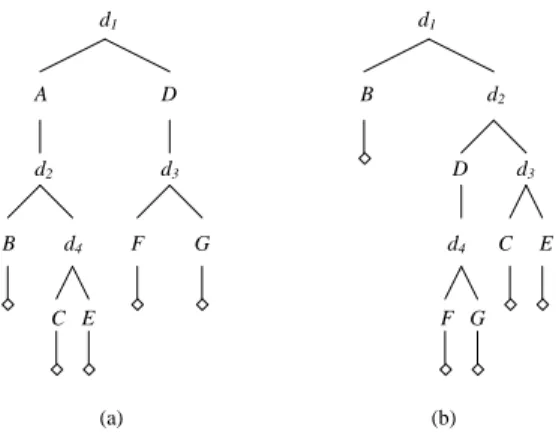
d1 d1 A D B d2 d2 d3 D d3 B d4 F G d4 C E C E F G (a) (b)
Figure 2: (a) An example purchase procedure tree. (b) The new purchase procedure built if A is pur-chased.
Auctions are sorted by finish time (earliest to latest). The set of products auctioned on a path in the tree uniquely corresponds to a bundle in B, and all elements of B are represented by some path. Figure 2 depicts two examples. Starting at the root node, the buyer proceeds toward the leaf nodes, bidding in auctions at auction nodes and making decisions at decision nodes. Auction nodes are represented by upper case letters and decision nodes by lower case d’s. At each decision node there are two choices: participating in the auction that will end next, which is always represented by the left child of the decision node, or allowing it to pass. When the auction ends, if the buyer is the winner then ex-ecution moves through the left child (which represents the auction just won), else execution moves to the right. Once a terminal node is reached, the buyer will have procured a complete bundle.
The example PPT in Figure 2(a) represents the problem where there are bundles B = {AB, AC, AE, DF, DG} and the auction for A ends first. The current decision (d1) to
be made is whether or not to bid on A. The PPT shows the consequential decisions and auctions which result from each choice. Note that a new PPT is built for each decision. For example, if A is purchased and D ends before C, the tree in Figure 2(b) would be built. The new tree would also include any new options that may have arisen. Note that this tree still contains bundles that do not include A, since it may be possible that such products could be so valuable or obtainable cheaply enough to justify their consideration, even if their acquisition could mean that A would be wasted.
4.
MODELING THE PROBLEM AS A
MAR-KOV DECISION PROCESS
To determine the expected utility of each option, the se-quence of auctions and decisions is modeled as a Markov de-cision process (MDP), and the optimal policy in the MDP is determined using the value iteration method of dynamic pro-gramming. Each state in the MDP is a 5-tuple hP, c, Acur,
cb, ti where P is the set of purchased products, c is the total
amount spent on purchases, Acuris the set of auctions that
are currently running, cb : Acur→ < maps each auction in
Acurto its current bid, and t is the time. The set of actions
is Q = {bid, notbid}. Each terminal state has an associated
reward, equal to the utility u(b, c) of purchasing the bundle
b = P at cost c. The value v(s) for a state s is computed as
the expected utility of s. The problem is to determine v(s) for each reachable state s in order to find the optimal policy
π : S → Q. For a state s0at which a bidding decision must
be made, π(s0) advises the course of action, either bidding
or not bidding, that maximizes expected utility.
Because of the stochastic nature of auctions, for many ac-tions it is not known for certain what the next state will be. However, we assume that the buyer will have some idea of what the outcomes of an auction will be (by examin-ing auction history, market history, estimation of competi-tors reserve values, etc.). We model this information in the form of a prediction function Fa(c, t, t0). For an auction a,
Fa(c, t, t0) takes a bid c and times t and t0 (where t < t0),
and returns a probability distribution p on the outcomes for the current bid at time t0 given that the current bid at time
t is c.
4.1
Reducing the State Space
The problem with modeling the decision problem in this way is that there will be too many states in the MDP for solution to be computationally feasible. At any given time, there may be several auctions open, each of which with sev-eral possible outcomes for the current bid. Also, there may be several different combinations of items already purchased by the buyer, and several possible costs for those purchased goods. An important contribution of this paper lies in how we deal with this computational complexity without losing too much of the important information. Three methods that can be used together to reduce the size of the state space are demonstrated. Note that our model still works when these restrictions are not in place. However, it is likely to be unrea-sonably slow for any interesting set of auctions. Therefore we show how the state space can be significantly reduced in such a way that the resulting MDP is still powerful enough to produce good results. In section 5, we show that our re-duced model can work significantly better than adaptations of other techniques from the literature.
4.1.1
Reducing the Set of Time Points
The first reduction method reduces the set T of time points to contain only those points where an auction is about to end. Specifically, T = {fa | a ∈ A}. Thus the model
assumes that the agent will only choose to bid in an auction at the very end. Since this will be the last bid, if the agent bids, it wins. Realistically, with this strategy the bidder runs the risk of not having a bid accepted before the deadline if there are one or more bidders attempting to bid at the same time, otherwise it would be the optimal strategy. But this is not necessarily the true strategy to be used by the buyer. It is only the assumption made about future actions in the MDP model to ease the computational burden. The buyer is free to bid earlier in an auction if the expected utility of doing so is higher than the expected utility of waiting until the end. As a result, since the utility of winning an auction with an earlier bid is always at least as good as winning it with a later bid (since bids never go down), the buyer’s true expected utility is at least as high as that predicted by the algorithm (given that the prediction functions are sufficiently accurate).
71 71
Outcome xi p(xi)
x1 = the x such that P (X > x) = .95 .185 x2 = the x such that P (X > x) = .5 .63 x3 = the x such that P (X > x) = .05 .185
Table 1: Outcomes for the PT three-point approxi-mation
4.1.2
Using the Purchase Procedure Tree
The PPT shows the sequence of decisions and auctions that follow from any choice. States in the MDP can be envisioned as occurring at some point in the tree. For example, in the PPT in Figure 2(a), any state with purchased products
P = {A} and time t = fB can be thought of as occurring
at decision node d2, since these are possible states that the
buyer could occupy when a decision on whether or not to buy B is being made. The PPT is used to reduce the state space in two ways. First, for any state s at that can occur at node n in the PPT, the set P in s is always equal to the set of ancestor purchases in the PPT. Thus we would never consider a state at time fB where both A and D had been
purchased, for example. It might still be possible to reach such a state, but it is unlikely since no bundle contains both
A and D.
Second, an auction a is in Acurin a state s at time t only if s
occurs at some decision node d, d is an ancestor of the node representing a, and a is running at t. Thus, when a deci-sion is being made, only the current bids are considered for auctions that appear as descendents of that decision node. For example, if the auctions running when the decision at
d3 needs to be made in Figure 2(a) are C, F and G, only
the current bids for F and G would be considered.
4.1.3
Reducing the Number of Bid Outcomes
The number of possible current bids for a set of auctions can be quite numerous. For example, if the possible current bid for an auction at a given time could be any integer be-tween 101 and 200, then there are 100 different outcomes. If there are 10 similar auctions open at the same time, then there are 10010possible joint outcomes for the current bids
in these auctions. The number of states in the MDP can be greatly reduced by reducing the number of possible bid out-comes. To accomplish this, we employ the Pearson-Tukey three-point approximation (PT-approximation) [9, 11]. The approximation works as follows. For a random variable X the space of outcomes is reduced to {x1, x2, x3}, each with
probability p(xi) as given in Table 1.
The PT-approximation is used to limit the number of out-comes given by the prediction function that will have posi-tive probability. Let pta(c, t, t0, i) be a function that takes a
bid c, times t and t0, and an integer i ∈ {1, 2, 3}, and returns
outcome xiat t0 according to Table 1, given that the bid at
t is c. These values are found using the probability
distri-bution given by the prediction function Fa(c, t, t0), inducing
a new prediction function F0
a(c, t, t0) = p0 where p0 assigns
positive probabilities to the three PT-approximation values. The set of possible outcomes using the PT-approximation for the current bid in an auction at a given time is deter-mined as follows. Let {t0, t1, . . . , tm−1, tm} be the set of time
100
105 120 130
110 125 138 125 145 160 136 171 190
Figure 3: A tree giving the set of possible current bid outcomes specified by F0
a
points that occur during an auction a represented by node
n in the purchase procedure tree, where t0 = sa, tm = fa,
and t1, . . . , tm−1are the decision times for ancestor decision
nodes of n. The set C(a, n, ti) of possible outcomes for the
current bid at time ti is as follows:
C(a, n, ti) = {c0} if i = 0 {pta(c, ti−1, ti, j) | c ∈ C(a, n, ti−1), j = 1, 2, 3} if 1 ≤ i ≤ m C(a, n, tm) if m < i (1) where c0 is the starting bid for a. For example, consider an
auction with starting bid of 100 and an example prediction function Fa. Also assume that the auction starts at time
0 and ends at 2. The possible outcomes for current bids can be viewed as a tree, as given in Figure 3. 100 is for sure the current bid at time 0. This particular prediction function Fa dictates that if 100 is the bid at time 0, then
at time 1 there is a 5% chance the leading bid will be 105 or below, a 50% chance it will be 120 or below, and a 5% chance it will be 130 or higher. Thus, F0
a(100, 0, 1) = p01 where p0 1(105) = .185, p01(120) = .63 and p01(130) = .185. In a similar fashion, F0 a(105, 1, 2) = p02 where p02(110) = .185, p0
2(125) = .63 and p02(138) = .185 (as given by the children
of 105). Thus there are at most three possible outcomes at time 1, and at most nine possible outcomes at time 2.
4.2
Specifying the Reduced State Space
Given these reduction techniques, we formally specify the state space for the MDP as follows. Each state is a 5-tuplehP, c, Acur, cb, ti where P is the set of purchased products,
c is the total amount spent on purchases, Acuris the set of
auctions that are currently running, cb is a mapping from
Acurto their current bids, and t is the time. The state space
S is determined by finding the possible states at each time t, which is done as follows. Let N be the set of decision
and/or terminal nodes in the purchase procedure tree such that each n ∈ N has critical time (decision or termination time) equal to t. Let Sn
t be the set of states that the bidder
can occupy at node n in the purchase procedure tree. The set St of states that include t is then the union of the sets
Sn
t for all n ∈ N . Then
where P , C, Acur, CB and t are as follows:
• P is the set of purchased products (i.e. the set of
products that label auction nodes on the path from the root to n in the tree). P is common in all states in Sn
t.
• C is the set of possible outcomes for the total cost
of purchased products. Let cprebe the amount spent
on products purchased before the root decision time (i.e. money already spent). Then c ∈ C if c is the sum of cpreand possible outcomes for the winning bids
for products in P . To state more formally, for each
pj ∈ P = {p1, . . . pm}, let nj be the node in the PPT
associated with pjand let aj be the auction. Then
C = {cpre+ m X j=1 cj| (c1, . . . , cm) ∈ C(a1, n1, t)× C(a2, n2, t) × . . . × C(am, nm, t)} (3)
• Acur is the set of pertinent auctions. The pertinent
auctions for a node n at time t are those auctions that are running at t and are represented by descendents of
n in the PPT. Thus these are the important running
auctions. More formally, a ∈ Acur iff a starts before t
and the node representing a is a descendent of n. Acur
is common in all states in Sn t.
• CB is the set of all possible mappings from Acur to
their possible current bids at t. That is,
CB = {cb | cb(aj) = cj where
(c1, . . . , cm) ∈ C(a1, n1, t) × . . . × C(am, nm, t)}
(4)
• t is the time.
The set St is then the union of all Snt, and the state space
for the MDP is thus the union of all St.
Since many possible states are eliminated from the MDP, it is likely the agent will find itself in states for which an action is not specified by the optimal policy π. However, since constructing a new MDP with the current state as the initial state will be much faster as a result of this reduction, it can be done in real time each time a decision needs to be made. The action specified by the optimal policy for the current state is then advised.
4.3
The Transition Probability Function
The transition probability function P r(s0|s, q) takes statess and s0 and an action q and returns the probability of
oc-cupying s0 directly after q is performed in s. In the PPT,
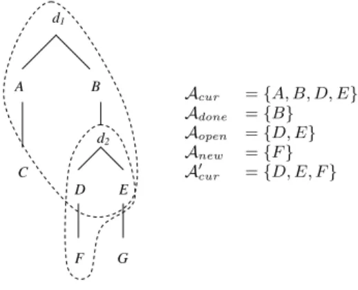
if the agent chooses to bid at a decision point, then the product is purchased and execution would move to the left child. Otherwise execution would move to the right child. d1 A B d2 C D E F G Acur = {A, B, D, E} Adone = {B} Aopen = {D, E} Anew = {F } A0 cur = {D, E, F }
Figure 4: An example partial purchase procedure tree where Acur, Adone, Aopen, Anew and A0cur are
in-dicated.
Let s = hP, c, Acur, cb, ti be a state and let d1 be the node
in the tree where s would take place. Let d2 be the node in
the tree where the next state is encountered after the action
q is performed in s. Let t0 be the time for the states that
occur at d2. Let Adonebe the auctions that are represented
by nodes on the path from d1 to d2 (i.e. the auctions that
the buyer will buy from as a result of the action taken), let
Aopen be the auctions that were pertinent and open at d1
and are still pertinent and open at d2 (i.e. are descendents
of d2), and let Anewbe the products for new pertinent open
auctions (i.e. for each a ∈ Anew, a starts after t and its node
is a descendent of d2). Figure 4 depicts an example partial
purchase procedure tree where Acur, Adone, Aopen, Anew
and A0
cur are indicated. Dashed lines enclose the auctions
that will be running when the decision node at the top of the enclosure is encountered. Finally, let α be a mapping from
Adone∪ Aopen∪ Anew to {1, 2, 3}. Then P r(s0|s, q) assigns
positive probability to s0= hP0, c0, A0
cur, cb0, t0i where
• P0 is the set of products purchased before d
2 is en-countered. • c0= c + X a∈Adone pta(cb(a), t, t0, α(a)). • A0
cur is the set of open auctions pertinent at n0 (i.e.
A0
cur= Aopen∪ Anew).
• cb0gives a new current bid for all auctions in A
open∪
Anew where cb0(a) = pta(cb(a), t, t0, α(a)) for all a ∈
Aopenand cb0(a) = pta(c0, sa, t0, α(a)) for all a ∈ Anew
• t0is the time at d
2
The probability of s0 resulting from performing action q in
s is
P (s0|s, q) = Y a∈Aall
zα(a) (5)
where Aall= Adone∪ Aopen∪ Anew and z1= .185, z2= .63
and z3= .185.
73 73
4.4
Rewards
Rewards are associated only with terminal states. When an entire bundle b is purchased, the reward is the utility of buying b for the total cost c. We assume the use of the von Neumann-Morgenstern theory of utility [14], and use the bilinear two-attribute utility function as given by Keeney and Raiffa [10]:
u(b, c) = kbub(b) + kcuc(c) + kbcub(b)uc(c) (6)
where ub : B → < and uc : C → < are the buyer’s utility
functions for bundles and costs, respectively, and kb, kcand
kbcare scaling constants.
4.5
The Dynamic Programming Model
The value iteration method of dynamic programming is used to determine the optimal action at each state. This optimal action is the one that maximizes expected value (in this case value is utility). Let v : S → < be the value function that assigns to each state its value, let π : S → Q be the optimal policy and let s = hP, c, Acur, cb, ti be a state. Then
v(s) = u(P, c) if P ∈ B max q∈{bid,notbid} X s0∈S v(s0)P (s0|s, q) otherwise (7) and π(s) = null if P ∈ B arg max q∈{bid,notbid} X s0∈S v(s0)P (s0|s, q) otherwise (8)
5.
RESULTS
Testing was performed on a set of auctions with the goal of demonstrating how well our algorithm (referred to here-after as the “tree-based” algorithm) performs with varying information available at each decision point. The algorithm was tested against adaptations of two algorithms from the literature. The first algorithm is an adaptation of that used by Byde et al. [7]. While their model allows for multiple simultaneous bidding in several types of auctions, when de-termining the expected utility of a choice it does not consider information over future decisions. The algorithm advises an agent to bid in an auction simply if that auction is part of the set of auctions that will yield the bundle with greatest expected utility. Since the algorithm tends to pursue the op-tions that are deemed to be the best at that given moment, we refer to this as the “greedy” algorithm1. The second
al-gorithm is an adaptation of that proposed by Boutilier et al. [3]. In their model, only sequential auctions are consid-ered, and thus there are never any other auctions running each time a bidding decision is made. Also, all auctions are first-price sealed-bid. The algorithm uses dynamic pro-gramming to determine the bid amount for each auction that maximizes expected utility, given the auctions that follow. We adapt this algorithm to our model as follows. First, rather than determine the optimal bid, since auctions are
1Note that their algorithm does however allow for
simulta-neous bidding, which we do not allow here.
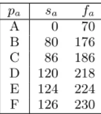
pa sa fa A 0 70 B 80 176 C 86 186 D 120 218 E 124 224 F 126 230
Table 2: Initial start and finish times for auctions in testing
open-cry in our model dynamic programming is used to de-termine the maximum bid such that the expected utility of bidding is greater than the expected utility of not bidding, given the auctions that follow. Second, auction start times are considered to be later to avoid overlaps. For example if auction a runs from time 10 to 20 and auction b runs from time 15 to time 30, if b is the next auction to finish after a then we act as if the auction for b runs from 20 to 30. Note that in testing, if a bidding decision is made on a while b is running, the current bid for b is considered and the ex-pected outcome is computed accordingly. The fact that they overlap is just not considered when looking at future deci-sion points. This algorithm is referred to as the “sequential” algorithm.
Tests were run using the product set P = {A, B, C, D, E, F } and the bundle set B = {AB, CE, DF }. The initial auc-tion times for the various products are given in Table 2. The purchase procedure tree is shown in Figure 5. An agent employing each algorithm was tested against 8 dummy agents who had reserve price and start time chosen at ran-dom for each auction. Bundle utilities for experiments were set at u(AB) = .5, u(CE) = u(DF ) = .53, utility for money uc(c) = 260−c100 and overall bundle utility u(b, c) =
.5ub(b)+.5kcuc(c). Dummy reserve values were chosen from
various distributions with mean $100, and the times at which they commenced bidding were chosen uniformly over the span of the auction. Dummy activity was initially observed for each auction so the agents could learn the prediction function. Fixed-increment bidding (i.e. agents always sub-mit the minimum bid) was used in auction simulations. The hypothesis of the test was that the tree-based method would perform better in relation to the other methods as the time period for auction C was moved later. As C is moved later, information as to the eventual outcomes for the auctions for D, E and F becomes more certain, since the decision on whether to bid on C moves closer to the other auctions’ finish times. This changes the expected utility of not buying A, since the expected utility of not buying A is dependent on the consequential decision of whether or not to buy C. The consequences of incrementally pushing back
C’s start and finish time back 2 time points at a time are
demonstrated by the data in Table 3, and graphically in Figure 6.
A paired t-test indicates that the tree-based algorithm per-forms better than the sequential algorithm with significance
p = .05 when C ends at 206 or later. The tree-based method
d1
A d2
B C D
E F
Figure 5: Purchase procedure tree used in tests.
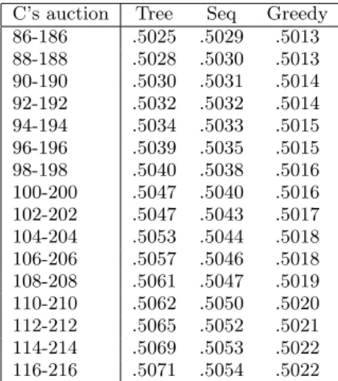
C’s auction Tree Seq Greedy
86-186 .5025 .5029 .5013 88-188 .5028 .5030 .5013 90-190 .5030 .5031 .5014 92-192 .5032 .5032 .5014 94-194 .5034 .5033 .5015 96-196 .5039 .5035 .5015 98-198 .5040 .5038 .5016 100-200 .5047 .5040 .5016 102-202 .5047 .5043 .5017 104-204 .5053 .5044 .5018 106-206 .5057 .5046 .5018 108-208 .5061 .5047 .5019 110-210 .5062 .5050 .5020 112-212 .5065 .5052 .5021 114-214 .5069 .5053 .5022 116-216 .5071 .5054 .5022
Table 3: Average utility achieved by each method over 2000 runs for each auction period for C. Tree-based algorithm performs better than sequential at significance level p = .05 when C ends at 206 or later. Tree-based performs significantly better than greedy for all C.
0.498 0.499 0.5 0.501 0.502 0.503 0.504 0.505 0.506 0.507 0.508 186 190 194 198 202 206 210 214 Finish Time for C's Auction
U ti li ty A c h ie v e d Tree Seq Greedy
Figure 6: Graphical representation of the data from Table 3.
C at p = .05. Notice however that the tree-based method
seems to perform worse than the sequential method when
C finished earlier than 192. This is because not enough
in-formation will be known at C’s decision point to give the based method the advantage. In fact, since the tree-based method uses approximation techniques, when this is the case it will estimate the expected utility less accurately than the sequential algorithm, and thus make poor deci-sions. Thus the tree-based algorithm can be quite powerful, but should be used only when sufficient information will be known at future decision points.
6.
SCALABILITY
The number of states in the MDP, given the reductions dis-cussed in section 4.1, is equal to the sum of the states that can occur at each decision and terminal node. For a termi-nal node n with termination time t, the possible states are
Sn
t = {P } × C × {Acur} × CB × {t}. Since P and t are
com-mon in all states in Sn
t, and Acur= φ and thus CB contains
only one (empty) function, then |Sn
t| = 1 × |C| × 1 × 1 × 1
and is thus bounded by the number of possible outcomes for the auctions for P .
If n is a decision node with decision time t, since P , t and Acur are common in all states in Stn, then |Stn| =
1 × |C| × 1 × |CB| × 1. |CB| is equal to the number of joint outcomes for all auctions in Acur at t, which is
deter-mined as follows. For each ai∈ Acur, let xibe the number
of ancestor decision nodes d of n such that ai begins
be-fore d’s decision time occurs. Then by equation 1, ai has
at most 3xi possible outcomes at time t, according to the
PT-approximation. The number of joint outcomes for all
ai∈ Acur is then less than or equal to
|AYcur|
i=1
3xi= 3P|Acur |i=1 xi (9)
and thus the number of possible states at a node n with occuring at time t is
|Sn
t| ≤ |C| × 3
P|Acur |
i=1 xi (10)
where C is the set of possible total costs for the items repre-sented by ancestors of n in the PPT, and xi is the number
of ancestor decision nodes d of n such that aibegins before
d’s decision time occurs. Thus the algorithm scales well as
the number of auctions increases, as long as |Acur| and/or
xistay small. As |Acur| and xigrow, the MDP can become
unmanageably large and approximation techniques such as the use of factored MDPs (see Boutilier et al. [1] or Guestrin et al. [8], for example) may be needed.
7.
RELATED WORK
Research on bidding decisions and strategies in multiple on-line auctions has been a growing field in recent years. New problems induced by the possibility of monitoring and par-ticipating in several auctions at a time have stretched the
75 75
limits of classical auction theory, and have been moving into the domain of computer science. As discussed previously, the idea of using dynamic programming to make bidding de-cisions was used by Boutilier et al. [2, 3] to determine how much to bid where the products were auctioned in sequence. Those authors also considered the problem of purchasing bundles, however in their model no auctions overlapped. In order to formulate distributions of the bid outcomes, they also examine multi-round auctioning where bid distributions can be learned over time. Byde [6] used dynamic program-ming to make bidding decisions in simultaneous auctions where the bidder is only interested in obtaining a single product. Byde et al. [7] analyzed the problem of determin-ing the optimal set of auctions for purchasdetermin-ing multiple units of a single product, and Preist et al. [12] gave a method that determines the optimal set of auctions when bundles of products are needed, and simultaneous bidding in multiple auctions is permitted.
8.
CONCLUSIONS AND FUTURE WORK
In this paper we present an effective algorithm for mak-ing biddmak-ing decisions in multiple English auctions where the buyer needs to procure one of possibly several bundles of products. We accomplish this by modeling the problem as a Markov decision process (MDP), and use a dynamic pro-gramming algorithm to find the optimal action at each de-cision point. To ease the computational burden, we reduce the number of states in the MDP by limiting the number of decision time points, enforcing the Pearson-Tukey three-point approximation on the transition probability function, and utilizing a purchase procedure tree to determine ex-actly what needs to be analyzed at each state. The dy-namic programming algorithm determines the expected util-ity of each choice (whether to bid or not to bid) based on the expected utility the bidder would have at consequen-tial decision points. We compare our method with adapta-tions of two algorithms from the literature, and show that our method performs significantly better when future bid-ding decisions will be made when the results of auctions are known with more certainty. Our algorithm uses the knowl-edge of this future information availability and more accu-rately determines the expected utility of current options. This results in better decision-making.
For future work, we plan to test our method on sets of actual online auctions, such as eBay. This will involve monitoring auctions for a period of time in order to determine a pre-diction function for similar future auctions, and then simu-lating these real actions with our bidding agent. This will give an idea not only of how well our technique performs in real auctions, but also how accurately these prediction functions can be determined. We also plan to extend the model so that bids can be submitted to several auctions at the same time. Considering such possibilities will make the problem more computationally complex, but we have shown in this paper that such complications can be overcome with creative state-reducing techniques.
9.
REFERENCES
[1] C. Boutilier, T. Dean, and S. Hanks. Decision theoretic plannning: Statistical assumptions and computational leverage. Journal of Artificial
Intelligence Research, 11:1–94, 1999.
[2] C. Boutilier, M. Goldszmidt, and B. Sabata. Continuous value function approximation for sequential bidding policies. In the Fifteenth Annual
Conference on Uncertainty in Artificial Intelligence (UAI-99), pages 81–90, Stockholm, 1999.
[3] C. Boutilier, M. Goldszmidt, and B. Sabata.
Sequential auctions for the allocation of resources with complementaries. In the Sixteenth International Joint
Conference on Artificial Intelligence (IJCAI-99),
pages 527–534, Stockholm, 1999.
[4] S. Buffett and A. Grant. A decision-theoretic algorithm for bundle purchasing in multiple open ascending price auctions. In the Seventeenth Canadian
Conference on Artificial Intelligence (AI’2004), pages
429–433, London, ON, Canada, 2004.
[5] S. Buffett and B. Spencer. Efficient monte carlo decision tree solution in dynamic purchasing environments. In Proc. International Conference on
Electronic Commerce (ICEC2003), pages 31–39,
Pittsburgh, PA, USA, 2003.
[6] A. Byde. A dynamic programming model for algorithm design in simultaneous auctions. In
WELCOM’01, Heidelburg, Germany, 2001.
[7] A. Byde, C. Preist, and N. R. Jennings. Decision procedures for multiple auctions. In Proc. 1st Int
Joint Conf. on Autonomous Agents and Multi-Agent Systems (AAMAS’02), pages 613–620, Bologna, Italy,
2002.
[8] C.E. Guestrin, D. Koller, and R. Parr. Multiagent planning with factored MDPs. In 14th Neural
Information Processing Systems (NIPS-14), pages
1523–1530, 2001.
[9] D. L. Keefer and S. E. Bodily. Three point approximations for continuous random variables.
Management Science, 29(5):595–609, 1983.
[10] R. L. Keeney and H. Raiffa. Decisions with Multiple
Objectives: Preferences and Value Tradeoffs. John
Wiley and Sons, Inc., 1976.
[11] E. S. Pearson and J. W. Tukey. Approximating means and standard deviations based on distances between percentage points of frequency curves. Biometrika, 52(3-4):533–546, 1965.
[12] C. Preist, C. Bartolini, and A. Byde. Agent-based service composition through simultaneous negotiation in forward and reverse auctions. In Proceedings of the
4th ACM Conference on Electronic Commerce, pages
55–63, San Diego, California, USA, 2003.
[13] T. Smith. eBay and your IT supply chain. TechWeb’s Internet Week, April 12, 2002, url =
“http://www.internetweek.com/story/showArticle.jhtml ?articleID= 6406064” (accessed on December 10, 2003), 2002.
[14] J. von Neumann and O. Morgenstern. Theory of
games and economic behaviour, 2nd ed. Princeton