Propulsion and maneuvering model tests of the USCGC Healy in ice and correlation with full-scale

(1)

Publisher’s version / Version de l'éditeur:

Questions? Contact the NRC Publications Archive team at

https://publications-cnrc.canada.ca/fra/droits

L’accès à ce site Web et l’utilisation de son contenu sont assujettis aux conditions présentées dans le site LISEZ CES CONDITIONS ATTENTIVEMENT AVANT D’UTILISER CE SITE WEB.

7th International Conference and Exhibition on Performance of Ships and

Structures in Ice [Proceedings], 2006

READ THESE TERMS AND CONDITIONS CAREFULLY BEFORE USING THIS WEBSITE.

https://nrc-publications.canada.ca/eng/copyright

NRC Publications Archive Record / Notice des Archives des publications du CNRC :

https://nrc-publications.canada.ca/eng/view/object/?id=015a8f4f-ab81-4b3c-8e30-df519dc60c0f

https://publications-cnrc.canada.ca/fra/voir/objet/?id=015a8f4f-ab81-4b3c-8e30-df519dc60c0f

NRC Publications Archive

Archives des publications du CNRC

This publication could be one of several versions: author’s original, accepted manuscript or the publisher’s version. / La version de cette publication peut être l’une des suivantes : la version prépublication de l’auteur, la version acceptée du manuscrit ou la version de l’éditeur.

Access and use of this website and the material on it are subject to the Terms and Conditions set forth at

Propulsion and maneuvering model tests of the USCGC Healy in ice

and correlation with full-scale

(2)

Propulsion and Maneuvering Model Tests of the USCGC Healy in Ice and Correlation with Full-Scale

Stephen J. Jones and Michael Lau

National Research Council of Canada, Institute for Ocean Technology, P.O. Box 12093, Stn. A, St. John’s, NL A1B 3T5. stephen.jones@nrc.ca

ABSTRACT

Propulsion model test results of the USCGC Healy are reported here and correlated with full-scale data. The design requirement for the Healy was for “continuous icebreaking at 3 knots through 4.5 ft (1.37 m) of ice of 100 psi (690 kPa) strength”. The full-scale trials were designed to test this capability. Unfortunately, the ice strength found on the trials was approximately half of that specified. One of the objects of the model tests was to determine the effect of ice strength on the delivered power necessary for the Healy to meet her icebreaking specification. Propulsion overload tests in open water combined with limited ice tests, and the IOT standard method for analyzing propulsion tests in ice, gave consistent results for delivered power, which agreed well with the available full-scale data from the Healy. A correlation friction coefficient of 0.05 was again shown to be appropriate. From the analysis of the resistance and propulsion tests, the Healy, with its total shaft horsepower of 30,000, was shown to be capable of its design requirement. Using a similar analysis, an imaginary “Polar 8” icebreaker of the Healy design was shown to require 85,000 HP to continuously break ice of 2.44 m (8 ft.) thickness, of 500 kPa strength, at 3 knots. Free running maneuvering tests performed in the ice tank gave arcs of circles whose diameters agreed well with the full-scale data of turning circles obtained on the ship trials.

KEY WORDS: USCGC Healy; ship performance; icebreaker; propulsion in ice; maneuvering in ice; ice-ship interaction

INTRODUCTION

Following the successful full-scale trials of the USCGC Healy in 2000, it was decided to conduct a complete set of resistance, propulsion, and maneuvering model tests of the vessel for correlation with the full-scale data. The proceedings of the POAC ’01 conference (Frederking et al. 2001) contain several papers outlining the results of the full-scale trials. Jones and Moores (2002), at the IAHR conference in Dunedin, have summarized the results of the resistance tests conducted at IOT. This paper details the propulsion and maneuvering model tests conducted at IOT and their correlation with the full-scale data.

USCGC HEALY

The USCGC Healy was launched on 15 November 1997 from Avondale Industries in New Orleans. She was delivered to the US

Coast Guard on 10 November 1999, departed New Orleans on 26th

January 2000, and proceeded north for extensive full-scale ice trials

before arriving in Seattle on 9th_{August 2000.}

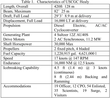
The essential details of the Healy are shown in Table 1. Table 1. Characteristics of USCGC Healy

Length, Overall 420ft 128 m

Beam, Maximum 82’ 25 m

Draft, Full Load 29’3’ 8.9 m at delivery

Displacement, Full Load 16,000 LT at delivery

Propulsion Diesel Electric, AC/AC

Cycloconverter Generating Plant

Drive Motors

4 Sultzer 12Z AU40S 2 AC Synchronous, 11.2 MW

Shaft Horsepower 30,000 Max

Propellers 2 fixed pitch, 4 bladed

Fuel Capacity 1,220,915 gal. 4,621,000 l

Speed 17 knots @ 147 RPM

Endurance 16,000 NM @ 12.5 knots

Icebreaking Capability 4.5 ft (1.4 m) @ 3 knots

(continuous)

8 ft (2.44 m) Backing and Ramming

Accommodations 19 Officer, 12 CPO, 54 Enlisted,

35 Scientists, 19 Surge, 2 Visitors

The design icebreaking capability of the Healy was for continuous icebreaking at 3 knots through 4.5 ft (1.37 m) of ice of 100 psi (690 kPa) strength. The full-scale trials were designed to test this capability. Unfortunately, the ice strength found on the trials was approximately half of that specified. One of the objects of the model tests was to determine the effect of ice strength on the delivered power necessary for the Healy to meet her icebreaking specification.

(3)

MODEL CONSTRUCTION

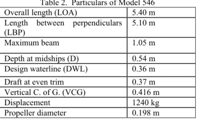
Model 546 was constructed, in accordance with IMD’s standard method, at a scale of 1:23.7. This scale was chosen so that we could use an existing set of propellers, namely our R-Class propellers 66L and 66R. The model’s principal dimensions were:-

Table 2. Particulars of Model 546

Overall length (LOA) 5.40 m

Length between perpendiculars (LBP)

5.10 m

Maximum beam 1.05 m

Depth at midships (D) 0.54 m

Design waterline (DWL) 0.36 m

Draft at even trim 0.37 m

Vertical C. of G. (VCG) 0.416 m

Displacement 1240 kg

Propeller diameter 0.198 m

A non-removable ice knife and two bossings, also non-removable, were fitted, together with the twin rudders and propellers. Fig. 1 shows the model in the ice tank.

ig. 1. Model 546 of the USCGC Healy in the ice tank at IOT.

e-hull friction coefficient

he ice-hull friction coefficient requested was 0.05. However, for

EST PLAN METHOD

ESISTANCE RESULTS

tance tests were conducted. Since the open water term a small contribution to the total icebreaking resistance, a least squares

ig. 2. iction.

evel Ice Resistance Results

Jones and Moores (2002) and will nly be summarized here. The standard IOT method breaks the total

= total resistance

breaking the ice

ice R

he end result t the resistance, one

r each ice-hull friction coefficient tested, from which the resistance F

Ic

T

unknown reasons, it was much smaller at 0.014 (Low friction) so the resistance tests were repeated after re-painting, at a friction coefficient of 0.034 (High friction). From these results, the resistance for a friction coefficient of 0.05 was extrapolated. The ice density was maintained

constant for the different ice sheets at 0.870 ± 30 Mg/m3.

T

overload tests, were conducted. The resistance tests were analyzed in accordance with IOT’s standard method (Standard # TM7) and the propulsion tests were analyzed in accordance with a draft standard method (TM 8 D1). Performance predictions were then made and compared to full-scale data previously collected. Further details of the test method can be found in an internal IOT report (Jones, 2004).

R

Open Water

Open water resis is

polynomial was fitted to the data and this was used to calculate the open water term as needed. Fig. 2 shows the result for the low friction model. This equation was used in order to subtract the open water term from the total resistance in ice.

F Open water resistance of the USCGC Healy model 546, low

fr

L

These results have been given in o

resistance down into four terms:-

OW B C BR T=R +R +R +R R where, R _T = resistance due to BR R

= resistance due to clearing the ice

C

R

= resistance due to buoyancy of the

B

R

W = resistance due to open water

O

T of he analysis is two equations for

fo

can be calculated for any value of ice thickness, strength, friction

100 y = 24.99x2 - 1.71x R2 = 0.997 0 20 40 60 80 0 0.5 1 1.5 2 2.5 Velocity m/s R e s is ta n c e N

(4)

( ) ( 2 M i i 6845 . 1 N 2 M i i 771 . 0 i M i i OW t BhV +0.866S BhV gh V 239 . 1 + T gBh 290 . 1 + R = R Δρ ρ ρ )

for the low friction (0.014) model and

( ) ( 2) M i i 771 . 1 N 2 M i i 642 . 0 i M i i OW t BhV +1.167S BhV gh V 035 . 1 + T gBh 138 . 1 + R = R Δρ ρ - ρ

-for the high friction (0.034) model.

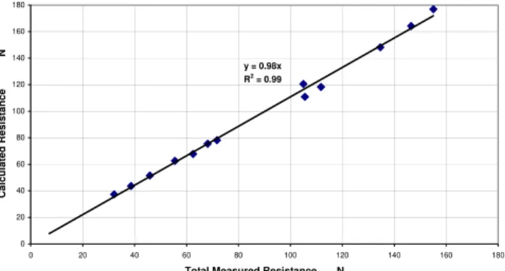
Fig. 3 demonstrates that the above equation (2) is indeed a good fit to the model data. A perfect fit would give a slope of 1.0.

Fig. 3. Calculated versus measured total resistance for the low friction, 0.014, Healy model.

Other resistance results obtained can be summarized as follows:- Effect of velocity on the total ice resistance, RIT = RT-ROW, can be best

fitted to a linear equation 1 49 + 5 68 = . v .

R_IT , where v is the velocity in m/s, and RIT is in N.

Effect of ice thickness can be best fitted to

i i

IT . h . h

R =002 2+135 , where hi is in mm and RIT in N.

Effect of friction was found to be best described as an increase of 15% in total ice resistance for an approximate doubling (from 0.014 to 0.034) in the friction coefficient.

Effect of ice strength was best described as a doubling of the ice

strength caused RIT to increase by 25% in thin ice (27mm) and 40% in

thick ice (76mm).

Further details of the resistance tests can be found in Jones and Moores (2002) and Jones (2005).

PROPULSION RESULTS

Propulsion tests were conducted according to IOT’s Standard Method TM8, D1.

Background and Theory of the Method

The principle of the method is that overload experiments in open water are used to predict the hydrodynamic torque required to develop a thrust sufficient to move the hull against a force equal to the hull

resistance in ice. Because such open water tests cannot take account of any ice-propeller interaction, it is necessary to conduct a corresponding experiment in ice to determine the increase in torque due to propeller-ice interaction. It is assumed in this method that propeller-propeller-ice interaction has a negligible effect on the thrust developed by the propulsion system. This has been shown to be true for small values of

hi/D where hi is the ice thickness and D is the diameter of the propeller

(Molyneux, 1989).

This method has certain advantages. If hydrodynamic effects can be separated from ice effects, some aspects of propulsive performance, for example, the effects of propeller pitch variation on tow force, can be investigated using only open water experiments. The torque due to ice can be considered as a function of the ice parameters (thickness, strength etc.) and added to the open water values. This method has the practical advantage that, because the towing carriage arrangement for resistance in ice tests and overload propulsion in ice tests are similar, it is possible to change quickly from one to the other. Thus, resistance and propulsion experiments in the same ice sheet are possible, provided that the propellers can be fitted or removed easily.

y = 0.98x R2 = 0.99 0 20 40 60 80 100 120 140 160 180 0 20 40 60 80 100 120 140 160 180

Total Measured Resistance N

C al cu lated R esi stan ce N

Self-propulsion tests in open water using an overload

method

The Healy model was equipped with the R-Class propellers, 66L and 66R. First, overload tow force tests were conducted in open water to give equations relating the tow force to rps for a given speed. The model was towed at a constant speed given by the carriage, and the rps was varied from 0 to between 12 and 18 rps depending on the speed. For a speed of 0.02 m/s the maximum rps was 12, for 1.2 m/s the maximum was 18 rps. The data were fitted to second order equations with high levels of accuracy. The results are shown in Fig. 4 below for the port side propeller. Similar equations were derived for the torque, Q, as a function of RPS, during these overload tests, as

Overload Tow Force

y = -1.0991x2_{+ 6.3992x + 33.985} y = -1.1487x2_{+ 5.9249x + 5.0078} y = -1.1015x2_{+ 3.5436x + 6.5797} y = -1.0762x2_{+ 1.6294x + 2.203} y = -1.0865x2_{+ 2.4328x + 2.8971} y = -1.0831x2_{+ 0.618x + 0.3834} y = -1.0762x2_{+ 0.2607x - 0.017} y = -1.0715x2_{+ 1.5881x - 1.655} -250 -200 -150 -100 -50 0 50 100 0 2 4 6 8 10 12 14 16 18 20 Port RPS [1/s] Tow Force [N ] 1.21 m/s 0.8 m/s 0.6 m/s 0.4 m/s 0.3 m/s 0.2 m/s 0.1 m/s 0.02 m/s

Fig. 4. Tow force in overload tests in of Healy model in open water

shown in Fig. 5. Neglecting ice-propeller interaction for the moment, it is now possible, therefore, to determine delivered power by:-

1. Equating resistance in ice for a specific ice thickness, strength, and speed to tow force from the open water overload tests

2. Determine an rps value from this tow force and Fig. 4.

(5)

4. Calculate PD from (2.π.Q.rps) and scale up for comparison

with full-scale.

5. Repeat for different values of ice thickness, strength, and ship speed.

Fig.5. Torque of port side propeller as a function of RPS for the open water overload tests.

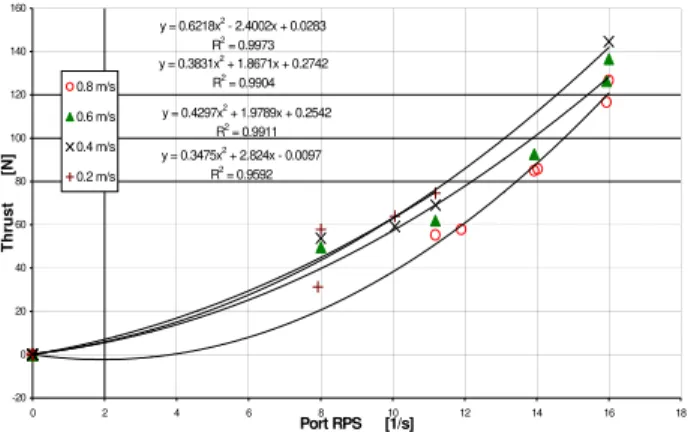
Propeller-ice interaction was taken account of as follows. Two ice

sheets were used for overload tests, one 39 mm thick and one 27 mm thick. Four speeds were used at five different rps. From these tests two

graphs were drawn as shown in Fig. 6 and 7. They show thrust, Ti, and

torque, Qi, plotted against rps. For a given set of ice thickness, strength

and ship speed, resistance can be calculated, equated to tow force and

an rps found from Fig. 4 above. From this rps, Q and Qi can be

calculated from Figs 5 and 7, and the ratio Qi/Q determined. A mean

value of this ratio is then determined and used to convert Q to Qi. From

this value of Qi, a value of Delivered Power is obtained and compared

to full-scale. The values of Qi/Q used are shown in Table 3 below.

Table 3. Values of Qi/Q used in the calculation of PD for model ice

thickness of 0.057 m and strength 15 kPa.

Model speed Ship speed Qi/Q

m/s kn 0.10 0.09 1.067 0.02 0.19 1.068 0.10 0.95 1.077 0.20 1.89 1.087 0.30 2.84 1.097 0.40 3.79 1.107 0.60 5.68 1.128 0.80 7.57 1.148 1.00 9.46 1.169 1.20 11.36 1.189 y = 0.6218x2_{- 2.4002x + 0.0283} R2 = 0.9973 y = 0.3831x2_{+ 1.8671x + 0.2742} R2 = 0.9904 y = 0.4297x2 + 1.9789x + 0.2542 R2_{= 0.9911} y = 0.3475x2 + 2.824x - 0.0097 R2 = 0.9592 -20 0 20 40 60 80 100 120 140 160 0 2 4 6 8 10 12 14 16 Port RPS [1/s] Thrust [ N ] 18 0.8 m/s 0.6 m/s 0.4 m/s 0.2 m/s y = -0.0151x2_{+ 0.0697x - 0.0043} y = -0.0145x2_{+ 0.0382x + 0.0002} y = -0.0153x2 + 0.0365x + 0.0064 y = -0.0119x2_{- 0.0082x - 0.0327} y = -0.0103x2_{- 0.0232x - 0.0309} y = -0.0105x2_{- 0.0237x - 0.0031} y = -0.0124x2_{+ 0.0021x + 0.0347} y = -0.0088x2_{- 0.0205x + 0.0064} -4.5 -3.0 -1.5 0.0 0 2 4 6 8 10 12 14 16 18 20 Port RPS 1/s Tor que Nm 1.21 m/s 0.8 m/s 0.6 m/s 0.4 m/s 0.3 m/s 0.2 m/s 0.1 m/s 0.02 m/s

Tared - Friction Values Removed

Fig. 6. Thrust developed during overload tests in ice, port side.

y = -0.0174x2_{+ 0.0604x + 0.0003} R2_{= 0.9929} y = -0.0111x2_{- 0.0332x + 0.0009} R2_{= 0.9964} y = -0.0126x2_{- 0.0174x - 0.0008} R2_{= 0.9995} y = -0.0158x2_{+ 0.0099x - 0.0003} R2_{= 0.9939} -6.0 -5.0 -4.0 -3.0 -2.0 -1.0 0.0 1.0 0 2 4 6 8 10 12 14 16 1 Port RPS [1/s] Tor que [N m ] 8 0.8 m/s 0.6 m/s 0.4 m/s 0.2 m/s

Fig. 7. Torque developed during overload tests in ice, port side.

Fig. 8 below shows the results of these calculations for the specific ice conditions of 1.36 m thickness and 351 kPa strength, which was the mean strength found during the full-scale trials for this thickness. The three “model” lines correspond to three friction coefficients; 0.014 and 0.034 as model tested, and 0.05 as extrapolated from the two others. The friction value 0.05 is the value that IOT has found gives best agreement between model-scale and full-scale, for a new hull in ice with little snow. The full-scale data was taken from Sodhi et al (2001) and was the delivered power measured independently on the propeller shafts by both torsion meters and strain gauges.

A shaft speed measurement system was also installed on each shaft. The shaft speed and torque measurements were then combined to determine the power delivered to each shaft. The two measurements of shaft torque agreed with each other within 1%.

(6)

Fig. 8. Delivered power for the Healy calculated from the model tests for three friction coefficients, the two experimental ones, 0.014 and 0.034 and extrapolated to 0.05, compared to the measured full-scale power. Ice conditions, 1.36 m thick of strength 351 kPa.

Good agreement can be seen in Fig. 8 between the model scale data for a friction coefficient of 0.05 and the full-scale data. Similar good agreement was found for the other ice thicknesses and strengths measured on the full-scale trials, although the power predicted from the model tests was always slightly lower than that measured at full-scale. Possible reasons for that are frictional losses in the ship’s shaft bearings aft of the point at which the power was actually measured, and the fact that we were not using true Healy propellers in the model tests, but stock R-Class propellers.

The Healy was designed for “continuous icebreaking at 3 knots through 4.5 ft (1.37 m) of ice of 100 psi (690 kPa) strength”. We have calculated, therefore, the delivered power required to do this, based on the model tests. The result is shown in Fig. 9 for the two friction coefficients tested and the 0.05 value extrapolated from them, in which it can be seen that the power required is just slightly greater than the 30,000 HP available on the Healy. Given the errors expected in both the full-scale and model-scale measurements of at least ±5%, we conclude that the Healy is capable of its design requirement.

For the sake of interest, we calculated the power required for an imaginary “Polar 8” icebreaker, assuming it to be identical in design to the Healy, as was proposed some

Fig. 9. Delivered power required for the Healy to break 1.37 m ice of 690 kPa strength calculated from the model tests.

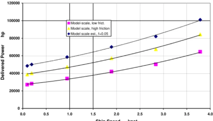
years ago in Canada. Fig. 10 shows the result for ice conditions of 2.44 m (8ft) of strength 500kPa. This shows that for continuous icebreaking at 3 knot in these ice conditions, a delivered power of about 85,000HP would be required. 0 5000 10000 15000 20000 25000 30000 35000 0 1 2 3 4 5

Ship Speed knot

De liv e re d Powe r hp 6 Full-Scale

Model scale, low frict. Model scale, high frict. Model scale, f=0.05 0 20000 40000 60000 80000 100000 120000 0.0 0.5 1.0 1.5 2.0 2.5 3.0 3.5 4.0

Ship Speed knot

D e liv e re d Powe r hp

Model-scale, low frict. Model scale, high friction Model scale est., f=0.05

Fig. 10. An imaginary “Polar 8” icebreaker of the Healy design for ice conditions 2.44 m thick and 500kPa strength.

MANEUVERING TESTS

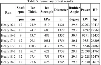
A total of 8 self-propelled maneuvering runs were conducted in three ice sheets. In addition, open water bollard (overload tests carried out at zero speed) and shaft friction tests were conducted. Selected test conditions from the sea trials were duplicated for the maneuvering tests and turning diameters were measured from the arcs of partial circles made in the ice tank. Performance predictions were then compared to the full-scale data previously collected. Table 4 shows the three ice sheets (in full scale units) that were used for the tests. Table 5 summarizes the test condition and the result for each run. The first three runs were conducted at a target ice thickness of 75 cm and an ice strength ranging from 483 to 683 kPa. Shaft speed was varied from 9 to 10 to 12 rpm for these runs. The remainder of the tests was conducted at a target ice thickness of 100 cm and an ice strength ranging from 417 to 1081 kPa. The rudder angle was kept at 30 degrees as used in the sea trials. The delivered power was kept at around 30000 hp, which was consistent with the delivered power employed during the full-scale trials.

Table 4. Details of ice sheets used

0 5000 10000 15000 20000 25000 30000 35000 40000 0.0 0.5 1.0 1.5 2.0 2.5 3.0 3.5 4.0

Ship Speed knot

D e liv e re d Powe r hp

Model-scale, low frict. Model scale, high friction Model scale est., f=0.05

Name Date Thick.

(cm) Strength (kPa) Density (Mg/m^3) E/σf Healy16 23 Nov 01 74 562 0.916 1938 Healy17 27 Nov 01 100 749 0.866 2156 Healy18 29 Nov 01 97 667 0.868 1256

(7)

Table 5. Summary of test results Shaft rpm Ice Thick. Ice Strength Diameter Rudder Angle Power HP Run rpm cm kPa m degree kW hp Healy16-1 12 74.9 519 1321 29.6 22703 30433 Healy16-2 10 74.7 683 1329 29.9 14592 19560 Healy16-3 9 73.7 483 1337 30.4 9291 12455 Healy17-1 12 99.1 1081 1756 30.1 19551 26208 Healy17-3 12 100.7 417 1757 29.9 18546 24860 Healy18-1 12 96.7 621 1738 29.7 23698 31767 Healy18-2 12 97.4 751 1738 29.6 24228 32478 Healy18-3 12 97.6 628 1745 29.8 23630 31676

Table 6. Summary of maneuvering data from the sea trial Test

Ice

Thickness Power Diameter Dia./B h/B Dia/L

# Cm HP m 000420_1740 87 20780 1538 61.5 0.0348 12.0 000421_1348 95 28377 1538 61.5 0.0380 12.0 000421_1901 95 28830 1388 55.5 0.0380 10.8 000506_0015 140 23848 1666 66.6 0.0560 13.0 000515_1258 132.5 29254 2174 87.0 0.0530 17.0 000515_1400 132.5 29414 2128 85.1 0.0530 16.6 000515_1532 70.5 27222 470 18.8 0.0282 3.7 000515_1532 70.5 23234 528 21.1 0.0282 4.1 000515_1532 70.5 23440 1142 45.7 0.0282 8.9 000515_1615 70.5 29299 1274 51.0 0.0282 10.0 Average 96.4 26370 1385 55.4 0.0386 10.8

The full scale data have been reported in by Sodhi et al (2001). They are summarized in Table 6 for completeness.

Comparison with full-scale data

Figure 11 shows the non-dimensional turning diameter as a function of the non-dimensional ice thickness for both the model and the full-scale data. Despite some discrepancy in ice strength and power level between the model tests and sea trial, the model data agree well with the sea trial data except for the three data points identified in the figure. These 3 points should be further investigated which were seen as outliers in the full-scale report.

A multi-variance regression of the turning diameter conducted for the eight test runs as a function of ice thickness, ice strength, and the power level gave the following equation:

D f i . . P h . . D= -2502+2167 -0226σ -00095 …(1)

where D is the turning diameter (in m), hi is the ice thickness (in cm), σf

is the flexural strength of ice (in kPa), and P is the power level (in

thought to be an anomaly due to applying a least squares fit to limited, somewhat scattered, data and for which the ice strength varied little.

ig 11. The dimensional turning diameter as a function of

non-ISCUSSION AND CONCLUSIONS

ropulsion overload tests in open water combined with limited ice tests

rom the analysis of the resistance and propulsion tests, the Healy is

n imaginary “Polar 8” icebreaker of the Healy design would require

preliminary analysis of the maneuvering test data showed a good

13.02 3.67 4.13 0 2 4 6 8 10 12 14 16 18 0 0.01 0.02 0.03 0.04 0.05 0.06

Ice Thickness/Beam Width Sea Trial IOT - HEALY16 IOT - HEALY17 IOT - HEALY18 Full Scale Average Power = 26370 HP Ship Length = 128 m Beam Width = 25 m Tur ni ng D ia m e te r/ S hi p Le ngt h F

dimensional ice thickness for the Healy sea trial and model test data

D

P

have demonstrated that the IOT Standard Method for analyzing propulsion tests in ice gives consistent results for delivered power, which agree well with the available full-scale data of the Healy. A correlation friction coefficient of 0.05 is again shown to give good agreement between model and full-scale..

F

shown to be capable of its design requirement of “continuous icebreaking at 3 knots through 4.5 ft (1.37 m) of ice of 100 psi (690 kPa) strength” with its 30,000 HP.

A

85,000 HP to continuously break ice of 2.44 m (8 ft.) thickness, of 500 kPa strength, at 3 knots.

A

correlation between the model test and sea trial results. Multi-variance regression was performed with the model test data and the result compared with selected full-scale measurements. The turning diameter obtained during the model tests was the same in one case and slightly larger than its counterpart measured at sea trial in another case. The three outliers associated with the sea trial results (identified in Figure 11) warrant closer re-examination of these data points. The hull friction, 0.034, used in the model tests was slightly lower than the target of 0.05. The effect of this discrepancy was not incorporated in the maneuvering analysis.

(8)