Analysis of weighted l̳₁-minimization for model based compressed sensing

Analysis of Weighted

fi-minimization

for Model

Based Compressed Sensing.

by

Sidhant Misra

B.Tech., Electrical Engineering

Indian Institute of Technology, Kanpur (2008)

MASSACHUSETTS INSTITUTE OF TECH4LOGY

MAR 10 2911

ARCHNES

Submitted to the Department of Electrical Engineering and

Computer Science

in partial fulfillment of the requirements for the degree of

Master of Science

at the

MASSACHUSETTS INSTITUTE OF TECHNOLOGY

February 2011

©

Massachusetts Institute of Technology 2011. All rights reserved.

A u th o

...

...

Department of Electrical Engineering and

Certified by ...

Computer Science

/ anuary 21, 2011

ablo A. Parrilo

Professor

Thesis Supervisor

Accepted by.

...

Terry P. Orlando

Chairman, Department Committee on Graduate Theses

Analysis of Weighted fi-minimization for Model Based

Compressed Sensing.

by

Sidhant Misra

Submitted to the Department of Electrical Engineering and Computer Science on January 21, 2011, in partial fulfillment of the

requirements for the degree of Master of Science

Abstract

The central problem of Compressed Sensing is to recover a sparse signal from fewer measurements than its ambient dimension. Recent results by Donoho, and Candes and Tao giving theoretical guarantees that (1-minimization succeeds in recovering the signal in a large number of cases have stirred up much interest in this topic. Subse-quent results followed, where prior information was imposed on the sparse signal and algorithms were proposed and analyzed to incorporate this prior information. In[13] Xu suggested the use of weighted fl-minimization in the case where the additional prior information is probabilistic in nature for a relatively simple probabilistic model. In this thesis, we exploit the techniques developed in [13] to extend the analysis to a more general class of probabilistic models, where the probabilities are evaluations of a continuous function at uniformly spaced points in a given interval. For this case, we use weights which have a similar characterization . We demonstrate our techniques through numerical computations for a certain class of weights and compare some of our results with empirical data obtained through simulations.

Thesis Supervisor: Pablo A. Parrilo Title: Professor

Acknowledgments

I would like to thank my advisor Pablo Parrilo for guiding me through my research. Through the numerous discussions we had, he gave me great insights and helped me learn several mathematical ideas and techniques.

I would like to thank my colleagues in LIDS for making the environment inspiring and enjoyable. I thank Parikshit Shah. Michael Rinehart and Mesrob Ohannessian for their useful advise and encouragement.

I am greatly thankful to Aliaa for her infinite support during the whole course of my masters. To my parents, I can never be thankful enough. Their unconditional love and encouragement has always been my guiding force.

Contents

1 Introduction

11

1.1

Compressed Sensing...

. . . . .

. . . .

11

1.2 Model-Based Compressed Sensing... . . . . .

. . . .

..

13

1.3

Organization of the thesis and Contribution . . . .

15

2 Background and previous work

17

2.1 The Ci-minimization method... . . . .

. . . .

17

2.1.1

Restricted Isometry Property...

. . . ...

18

2.1.2

Neighborliness of Randomly Projected Polytopes. . . . .

20

2.2

Iterative Recovery Methods... . . . .

. .

23

2.3

Model Based Compressed Sensing... . . . .

. . . .

25

2.3.1

Deterministic model.. . . .

. . . .

25

2.3.2

Probabilistic model.. .

. . . .

28

3 Weighted fi-minimization for a specific family of weights-

Formula-tion and Analysis

31

3.1 Derivation of Internal and External Angles... .

. . . .

..

32

3.1.1

Internal A ngle . . . .

33

3.2 Angle Exponents for a specific class of weights... .

. .

.

37

3.2.1

Internal Angle Exponent.. . . .

. . . .

38

3.2.2

External Angle Exponent . . . .

41

3.3

Derivation of the critical Threshold . . . .

43

3.4 Improving the Bound on the Exponents.. . . . . .

. . . .

46

3.4.1

Combinatorial Exponent... . . . .

. . . .

48

3.4.2

External Angle Exponent... . . . .

. ..

48

3.4.3

Internal Angle Exponent.. . . .

. . . .

49

3.5

Concavity of the Exponent Functions.

. . . .

.

51

3.6

Incorporating the probabilities in the derivation. . . . .

54

3.6.1

Bounding the probability of error and c-typicality....

. .

.

55

3.6.2

Exponents . . . .

62

4 Numerical Computations and Simulations

65

4.1

Behavior of FO under random projection.. . . .

. . . .

66

4.2 Performance of weighted el-minimization . . . .

69

5 Conclusion and Future Work

List of Figures

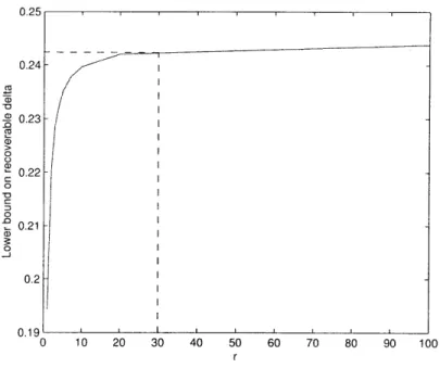
3-1 Maximum recoverable 6 vs r computed using the methods of this section. 51

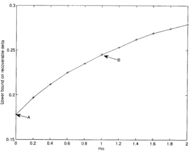
4-1 _{Lower bound on maximum recoverable J vs p for the "first face"' FO,}

computed using the methods developed in Chapter 3 for r = 30 . . . 67

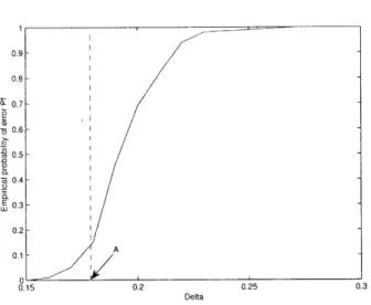
4-2 Empirical probability of error Pf vs 6 with p = 0 for FO obtained through simulations using in = 200, n = 400 and 100 iterations. The vertical line refers to the lower bound computed using methods of Chapter 3... ... 68 4-3 Empirical probability of error Pf vs 6 with p =1 for FO obtained

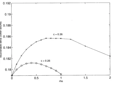
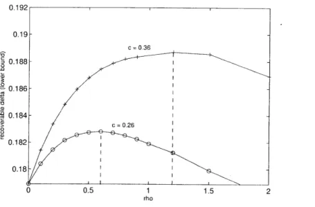
through simulations using in = 200. 1 = 400 and 100 iterations. The vertical line refers to the lower bound computed using methods of Chapter 3... ... 68 4-4 Lower bound on recoverable

o

vs p for ' = 0.5 computed using the

methods of Chapter 3, for c = 0.26 and c = 0.36. The parameter r is

fixed at 30. ... ... 70

4-5 Lower bound on recoverable 3 vs p for ! = 0.5 computed using the methods of Chapter 3, for c = 0.26 and c = 0.36. The parameter r is fixed at 60... . . . . . . ... 71

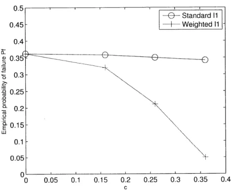
4-6 Empirical probability of error Pf vs c. Probability function p(u) =

0.185 - c(u - 0.5). Problem size is given by m

500, n

=

1000.

Number of iterations = 500... . . . . . . . . 72

Chapter 1

Introduction

1.1

Compressed Sensing

Compressed Sensing refers to obtaining linear measurements of a signal and com-pressing simultaneously and has been an area of much interest recently. Previously, the most common way to view recovery of signals from its samples was based on the Nyquist criterion. According to the Nyquist criterion for band-limited signals, the signals have to be sampled at twice the bandwidth to allow exact recovery. This is true for general band-limited signals but does not take into account any additional structure of the signal that might be known. In compressed sensing literature, the additional structure considered is that the signal is sparse with respect to a certain known basis. As opposed to sampling at Nyquist rate and subsequently compress-ing, measurements are now obtained by the action of linear operators on the signal. After fixing the basis with respect to which the signal is sparse., the process of ob-taining the measurements can be written as y = Ax. where. y E R"m is the vector of measurements.

x

C

R" is the signal and A E R"' " n represents the m linear

fune-tionals acting on the signal x. The signal x is considered to have at most k non-zero components. Compressed Sensing revolves around the fact that for sparse signals, the number of such linear measurements needed to reconstruct the signal can be significantly smaller than the ambient dimension of the signal itself. This recovery method aims at finding the sparsest solution x satisfying the constraints imposed by the measurements y which we represent by.

min ||x|o subject to y = Ax.

Note that this problem is inherently combinatorial in nature. For a certain value of the size of the support given by

k,

it involves searching through all possible

(k)

possible supports of the signal resulting in a NP-hard problem. Seminal work by Cand6s and Tao in

[5]

and Donoho in [7] show that under certain conditions on the linear operator in consideration, fi norm minimization, which can be recast as a linear program, can recover the signal from its measurements. The implication of this result is profound. Linear programming is known to have polynomial time complexity, and the above mentioned result tells us that for a large class of problems we can solve an otherwise combinatorial problem in polynomial time. Subsequently, iterative methods based on a greedy approach were formulated which recover the signal from its measurements by obtaining an increasingly accurate approximation to the actual signal in each iteration. Examples of these include CoSaMP [10] and IHT [3]. In Chapter 2, we will give a fairly detailed description of CoSaMP and its performance.

1.2

Model-Based Compressed Sensing

Most of the earlier literature on Compressed Sensing focused on the case where the

only constraints on the signal x are those imposed by its measurements y. On the

other hand it is natural to consider the case where apart from sparsity, there is

cer-tain additional information on the structure of the underlying signal known to us.

It would still of course be a valid approach to use some of the previously suggested

methods such as fe-minimization or CoSamp. but this would fail to exploit this

addi-tional information. It would be of interest to devise recovery methods specific to the

case at hand. Furthermore, one would also want to know if using the new recovery

method gives us benefits over the previous method (lesser number of required

mea-surements for the same level of sparsity of the signal). The authors in [2] introduced

a deterministic signal model. The support of the underlying signal under this model

is constrained to belong to a given known set. This defines a subset

M

of the set

of all k-sparse signals, which is now the set of allowable signals. This results in an

additional constraint on the original problem.

min |x|0

subject to y

Ax,

x

E M.

It turns out that a simple modification to the CoSamp or IHT actually succeeds in

exploiting the information about the model. The key property defined in [5], known

as the Restricted Isometry Property was adapted in [2] to a a model based setting.

With this, it was shown that results similar to [5] can be obtained for the

model-based signal recovery. The fact that the number of sparse signals in the model

M

is now fewer than the unconstrained case allows us to use lesser number of linear

measurements.

As opposed to this, Xu in [13] considers a probabilistic model. Under this model

there are certain known probabilities associated with the components of the signal

x. Specifically, pi, i = 1, 2..

n

with 0

<

pi < 1 are such that

P(xi is non-zero) =p

i =1 2..n.

Use of a weighted El-minimization as opposed to the standard El-minimization was suggested for this case. This can be written as

min ||IW||.1

subject to y = Ax,

where

||x|i

|

=1 = _1 w

jx

denotes the weighted f1 norm of x for a certain set of positive scalars wi,

i

1, 2 .... n. High dimensional geometry based ideas similar to those in [7] were used to provide sufficient conditions under which this linear program recovers the sparse signal. The specific model considered involves a partition of the indices 1 to n into two disjoint sets T and T2. The probabilities described above

are given by pi

= P

1

, i C T

1 and

pi =

P2.

i

C

T

2

. Naturally, the weights used are

w = W1, i E Ti and wi = W1, i E Ti. We will give a more detailed discussion on this in the next chapter.

1.3

Organization of the thesis and Contribution

In Chapter 2, we give a more comprehensive survey of the main results in Com-pressed Sensing literature, both for the standard and model-based case. Towards our contribution, in Chapter 3, we consider a more general probabilistic mode than in

(13).

Consider a continuous monotonically decreasing function p : [0, 1] - [0, 1]. Let the probability pi that the ith entry of x is non zero be given by

pA = p --.

The weighted 11-minimization for recovering x from the measurements y is as follows:

min ||x||,

(1.1)

subject to Ax = y. (1.2)

For this case, we consider the positive weights wi, which have a similar characteriza-tion

wi

=

f

-,

n

where

f

: [0, 1) -+ R is a continuous, positive and monotonically increasing function. The choice of a monotonically increasing

f(.)

for a monotonically decreasing p(.), is based on the intuition that we want to "encourage" the positions with higher prior probability to be more likely to be nion-zero by assigning lower weights to them. We generalize the proof machinery in

[13]

to provide sufficient conditions for success of the weighted e-minimization in our setting. In Chapter 4 we provide numerical and

simulation results, pointing out some of the salient features of our case. In Chapter

5, we conclude, with discussion on possible future works and interesting problems on

Chapter 2

Background and previous work

In this chapter we will describe some of the main results in Compressed Sensing. Most

of the results show that under certain conditions on the parameters of the problem,

comiputationally efficient methods such as el-minimization succeeds in recovering the

sparse signal from its measurements. It is difficult to prove such sufficient conditions

for general deterministic matrices. So. typically in the literature it is assumed that

the measurement matrix A is drawn from a random Gaussian ensemble, that is, the

entries of the matrix are i.i.d Gaussian random variables with mean zero.

2.1

The

e

1

-minimization method

In this section, we will present the seminal works of Candes and Tao

[5]

and Donoho

[7]

regarding the success of Er-minimization in recovering sparse signals from

underde-termnined systems. The approach in

[5]

is based on the so-called Restricted Isometry

Property which is the topic of the following section. In the subsequent section, we

will discuss the work in

[7),

based on the so-called neighborliness property of high

dimensional polytopes.

2.1.1

Restricted Isometry Property

Candes and Tao in

[5]

defined a notion of Restricted Isometry Property (RIP) for

matrices. The RIP is in a sense a weaker notion of orthonormality and stems from

the observation that in higher dimensions, two random vectors are nearly orthogonal

to each other. In the subsequent parts

||xI|

will be used to refer to the

f2

norm of

the vector x.

Definition 2.1.1.

[5]

Let A

C

R"'"m

be a matrix. For every integer 1 < k < n, the

k-Restricted Isometry constant

ok

is defined to be the smallest quantity such that

for all vectors x with

|supp(x)|

< k, A satisfies

(1

-

6k) Ix

2

||Ax||

2

< (1

+

6k) XII

Similarly, the ki, k

2

restricted orthogonality constant

Okik 2

for ki

+

k

2

< n is defined

to be the smallest constant such that, for any vectors

x1,

x

2

with disjoint supports

which satisfy supp(xi)j < k

1

and |supp(x

2)|

< k

2

, A satisfies

S(Ax

1

Ax2)

I

k,k2IIXIII

-

IX2I-The constants

ok

and 0

k,,k2 gives us an indication of how close the set of coluin

vectors of A are to being an orthonormal system. Of course for an exact orthonormal

system the vector x can be easily determined from its measurements y = Ax.

How-ever for sparse vectors. near-orthonorniality in the sense of the RIP suffices. This is

encapsulated in the following theorem.

Theorem 2.1.1. [5] Assume that

for

a given k, with 1

K

k < n, the restricted

isometry constants

satisfy

6

k + 0k,k + 0k,2k < 1.

Let x z R" be such that

|supp(x)|

< k, and let y = Ax. Then x is the unique solution

of

min ||x||1

subject to Ax = y.

While this theorem gives a sufficient condition for recovery, it is of interest to

know when is this condition satisfied. Now, for a system to be strictly orthonormal,

we must have m = n. Surprisingly, if the strictness is relaxed in the sense of the RIP,

it is now possible to have a much larger number of column vectors and still satisfy

the near orthonormality condition. Furthermore, matrices drawn from the random

Gaussian ensemble with certain conditions on its dimensions satisfy this property

with overwhelming probability.

Theorem 2.1.2. [51 Let A G R"xf with m < n be a matrix with entries that are i.i.d Gaussian with mean 0 and variance . Then there exists a constant 6*(m, n) such that if k = 6 satisfies 6 < 6 (m, n), then the conditions on the Restricted Isometry_n

Constants given in Theoren 2.1.1 are satisfied with overwhelming probability.

It turns out that the constant 6*(m,n) in the above theorem is such that for a

given level of sparsity k, we need only m = O(k log(n/k)) number of measurements

The Restricted Isometry based analysis turned out to be a powerful tool in Coni-pressed sensing and has been used extensively in subsequent work on the topic. Interestingly, it has been shown that recovery methods not based on E1-minimization can also guarantee recovery under certain conditions on the Restricted Isometry

Constants.

2.1.2

Neighborliness of Randomly Projected Polytopes.

In this section we present an overview of the high dimensional geometry based ap-proach introduced by Donoho to analyze the performance of f1-minimization. It revolves around the fact that the so-called neighborliness property of high dimen-sional polytopes has a strong connection to sparse solutions of underdetermined system of linear equations. Before proceeding, we provide a precise definition of this

neighborliness property.

Definition 2.1.2. [6] A polytope P is called k-neighborly if every set of k vertices forms a k - 1 dimensional face of the polytope. Similarly, a centrally symmetric polytope P is called k-centrally-neighborly if every set of k vertices not including antipodal pairs, form a k - 1 dimensional face of P.

Consider the unit fi-ball C defined by

C

=

{

Ec:

R"|IX

<1}.

For a given measurement matrix A, one can talk of a corresponding quotient polytope

P = AC which is the image of C under the transformation defined by A. The theorem

connecting neighborliness to recovery can then be stated as follows:

for

every xO E R"

with at

most

k non-zero

entries with

y =

Axo. xo is the unique

solution to the optimization problem.

imin

_||IIxi

subject to Ax = y.

When m < n and A has i.i.d. Gaussian entries, the polytope P can be interpreted as "a random projection" of the symmetric crosspolytope C C Rn onto a lower dimension m. One would expect that projecting onto a lower dimension would make the polytope "lose" faces. However it turns out that in higher dimensions, the lower dimensional faces "survive" with overwhelming probability. Therefore, it is of interest to characterize exact conditions under which this neighborliness holds. To this end, we need to define the face numbers of a polytope,

fi(C)

= the number of 1-dimensional faces of polytope C. The polytope P is then k-neighborly if and only if

f

1(AC)

f

1(C). I - 0.1, ... k - 1. We can now state the main Theorem in [7).

Theorem 2.1.4.

[7]

Let 0 < 6 < 1 be a constant. There exists a certain function

PN

(0,

1] -+ [0.

1).

such

that

for p

< pN(6

), and a uniformly distributed

random projection A

C

R""" with mn > n. we have

Pff(AC) =

fl(C),

1 = 0, 1,

...

pm} -+

1

as n

-4 oo.

To prove this central theorem, the author makes use of powerful results in high dimensional geometry. Affentranger and Schneider in [1] proved the following result.

Efk(AC) =

fk(C)

- 2

(

(

(F. G)y(G. C).

where Efk(AC) refers to the expectation over all possible projections and JK(C) denotes the set of all (k - 1)-dimensional faces of the polytope C. As there is a possibility that some of the k - 1-dimensional faces of C are "swallowed" up by the projection. we always have fk(AC) < fk(C). This in turn yields

P{fk(AC)

$

fk(C)} < fk(C)

-

Efk(AC)= 2Z

E

E

(F,G)>(G,C).

s>O FEJk(C) GEJ,,+i+2s(C)

The quantity

#(F,

G) is called the internal angle at face F of G and is the fraction of the unit hypershpere covered by the cone obtained by observing the face G from an internal point in F. For a given face G, -y(G, C) is called the external angle of the polytope C at the face G and is defined as the fraction of the unit hypersphere covered by the cone formed by the outward normals to the supporting hyperplanes of C at the face G. In [7] the author then proceeds by showing that these internal and external angles decay exponentially with respect to

n

whenever p

PN(6)-The quantity pN(6) is called the strong neighborliness threshold. PN(6)-The "strong" refers to the fact that below the threshold, all the k - 1-dimensional faces of C survive under the projection and the number fk(AC) is exactly equal to fk(C). This in turn guarantees that all k-sparse vectors x can be recovered by using El-minimization. Corresponding to this, Vershik and Sporyshev in [12], study a weaker notion of threshold in the same setting. They derive a threshold corresponding to approximate equality of face numbers. Formally this can be written as follows.

Theorem 2.1.5. Let 0 < 6 < 1 be a constant. There exists a certain function

p, : (0. 1] -s [0, 1], such that for p < pF,(

6

),. and a Uniformly distributed random

projection A G R"'x with m > 6n. Uc have

fi(AC) = fi(C) + op(1).

As will be described in the next section, this weak threshold is the one that will be useful when we consider probabilistic model based compressed sensing.

2.2

Iterative Recovery Methods

There have been some greedy-based algorithms that have been proposed to recover sparse signals from underdeterinined systems. CoSanip[10] , and IHT[3] are among such methods with comprehensive theoretical guarantees. These algorithms proceed by constructing an approximation to the solution at each iteration. We will describe the CoSaMP algorithm in detail.

CoSaMP[10

Initialization

Updating

u =A*v

Q supp(u2k),

T =

supp(azl) U Q

bT= A'Ty,be

= 0 a= bk v y - Aa'.

Here,

bT

is defined by

bT(j) - b(T).

1

j

<

TI,

Xk,

denotes the best

k-sparse

approximation in the least square sense to the vector x, and A+ is the pseudo-inverse

of the matrix A.

Note that if A were a perfectly orthonorinal system, the step u = A*v would

straight away give us back the vector x in the first iteration itself. Here, u serves

as a "good" estimate for x because of the near-orthonormality of A in the sense of

the RIP. Infact, the authors make use of an assumption on the restricted isometry

constants to guarantee that this algorithm converges and recovers the correct x. We end this section with the main theorem from [10]

Theorem 2.2.1.

[10J

Assume the matrix A satisfies 6

4k < 0.1, then the estimation ai at the end of the ith iteration satisfies

|i

-

ai112

2

-ki|xI2

+

20v

Here v refers to the so called unrecoverable energy which takes into account the

2.3

Model Based Compressed Sensing

In the previous two sections, we discussed about the basic compressed sensing prob-lem and presented the two primary approaches to efficiently recover sparse solutions to underdetermined systems. In the basic problem, the constraints on the signal x are only those imposed by its measurements, i.e. Ax = y. It is then natural to consider the scenario when additional information about the signal is known a priori. The question arises as to what kind of prior information is of interest and how do we in-corporate this prior information to our advantage. In the next couple of subsections, we will describe the two different kind of characterization of prior information that has been considered in recent literature and the corresponding suggested recovery methods and their performance.

2.3.1

Deterministic model

The authors in

[21

considered the case when there is a deterministic model imposed on the support of the k-sparse vector x. Using the terminology of

[21,

we give the definition of this model. Let

xIQ

denote the entries of x corresponding to the set of indices Q C {1, 2 .. , n}.

Definition 2.3.1. [2] A signal model Alk is defined as the union of mk canonical k-dimensional subspaces denoted by

Mk

Mk

U

Xi

{x.

X12 -

O}.

i-1

{

Q1,..., Qrmk} are the set of possible supports that define this model.

a simple modification to the CoSamp and IHT algorithms. Before we present the modified CoSamp algorithm, we first give a couple of definitions from [2].

Definition 2.3.2.

[2] For a positive integer

B,

the set

M

is defined as

B

M

{

x : X x',x

C

Mk.} r=1

Definition 2.3.3. [2] For a positive integer B, MB(x, k) is defined as

MB(x, k) = arg

min

I -

X 11

2

.

~MB

_k

which refers to the best model based Bk-sparse approximation to x.

The modification to the CoSamp Algorithm essentially involves replacing the best Bk-sparse approximations with the best model based Bk-sparse approximation. Surprisingly, this simple modification captures and exploits the information provided by the knowledge of the model very well.

Model Based CoSamp[2]

Initialization

Updating

i~i+1

u

A*v

Q supp(M2(u, k)), T = supp(ai- 1) U Q

bT = A+Ty,bT = 0

a'

=

M1(b,

k)

v = y - Aa.

Of course for the algorithm to be efficient, finding best model based approximation to a given vector should allow efficient computation. The performance guarantees of the above algorithm provided in [2] are very similar to those in [10], except that it

is now based on a model-based Restricted Isometry Property.

Definition 2.3.4. [2] (Model Based RIP -

Me-RIP)

A E R"nxn is said to have the MB restricted isometry property if there exists a constant 6_{,, such that for all}

£

E Mf,

we have

(1

-

8B)||xI|

2

<

||AxI|

2

<

(1

+ _AI)3)Ix||2

We now state the theorem in [2] corresponding to Theorem 3.2.1, giving sufficient conditions on recovery for the model based CoSamp.

Theorem 2.3.1. [21 Assume the matrix A satisfies

agf4 K

0.1, then the estimation

a at the end of the

ith iteration

satisfies

For a matrix A drawn from the random Gaussian ensemble to satisfy the model based RIP, we need m = O(k +log(mk)) [4]. For the unconstrained case (absence of any model), we have mk =

()

which gives m

= O(klog(n/k))

as before. This tells

us that for more restrictive models (smaller mk). we need much fewer measurements for recovering the signal if we use model based recovery methods (e.g. model based CoSAmp) as opposed to the standard methods for the unconstrained case.

2.3.2

Probabilistic model

In this subsection, we present in fair amount of detail the work by Xu in

[13].

Our work is based on the methodology that we will discuss subsequently. We mention the main steps of this methodology so that our work, which is the content of the next chapter, will be in continuation of what we present in this subsection.

In

[13],

the author considered that there is a set of probabilities pi, . . ,

p,

known

to us such that P{xi / 0} = p.. The use of weighted t1-minimization is suggested to recover x from its measurements y and is given by,

n

mm

in

wijxi|

subject to Ax = y.

Intuitively, we would use a larger wi corresponding to a smaller pi. We are in some sense improving the chances of recovery for those sparse vectors with higher proba-bility at the same time paying by reducing the chance of correct recovery for sparse vectors with low probability. By doing so we are aiming at enhancing the chances of recovery on an average. The notion of a strong threshold as described in the previous section is no longer applicable inthis case, because the strong threshold characterizes

the condition when all k-sparse x can be recovered. Also, the Restricted Isometry

Property defined in section 2.1 treats all k-subset of columns of A uniformly and thus

in its current form is not going to be useful in analyzing weighted E-minimization.

The author in [13] makes use of a method similar to the high dimensional geometry

approach in

[71,

but considers the notion of weak threshold. Herewe give a detailed

description of this notion.

Let P be the skewed crosspolytope given by {x E R I

||xfl|

1

< 1}. Without

loss of generality we can assume that the vector x has

||x||,

= 1. Let the support

set of x be

given

by

K

=

{ii i, 2 ... ik}.

We fix a particular sign pattern for

x,

say all positive. Then x lies on the k

-

1 dimensional face F of the cross polytope

P which is the convex hull of the vertices e,.

.

e,, where et denotes the vector

in R" with

_wiI

in the

ith

position and 0 everywhere else. As any solution to the

weighted ei-minimization problem satisfies Ax = b, the solution is of the form x

+u

where u belongs to the null space of A. The event that an incorrect solution is

obtained is precisely the event that there is a vector u in the null space of A such

that x + ul

< 1. The following lemma regarding the null space of a matrix with

i.i.d. Gaussian serves as a key observation.

Lemma 2.3.1. Let A

C R"x" be a random 'matrix with i.i.d.

N(0.

1) entries. Let

Z be a matrix of colurn vectors spanning the null space of A. Then, the distribution of A is rotationally invariant and it is always possible to choose a basis such that the entries of Z are distributed independently according to a normal distribution with mean 0 and variance 1.

This says that the null space of A is a random subspace and sampling from

this null space is equivalent to uniformly sampling from the Grassman manifold

probability of failure Pf, the probability that weigthed fi-minimization fails to

re-cover the correct x. Pf is the probability that a uniformly chosen n

-

m dimensional

random subspace shifted to the point x on the face F intersects the crosspolytope P

non trivially at some other point other than x. This is the so called complementary

Grassmann Angle for the face F with respect to the polytope P under the

Grass-mann manifold Gr(n-m)(n). Based on work by Santalo [11] and McMullen [9] the

Complementary Grassmann Angle can be can be expressed explicitly as the sum of

products of internal arid external angles as follows.

Pf

=

2Y

E

(F, G) -y(G, P)

(2.1)

s>O GEJ(m+1+2s)

where O(F, G) and -y(G, P) are the internal and external angles defined previously.

The author in [13] then proceeds by bounding the exponential rate of decay of the

in-ternal arid exin-ternal angles, to characterize the conditions under which the probability

of failure Pf goes to zero with overwhelming probability. Much of this technique is

suitably adapted to our case and will be presented in full detail in the next chapter.

Chapter 3

Weighted

fi-minimization

for a

specific family of

weights-Formulation and Analysis

In this chapter, we consider the problem of model based compressed sensing with a probabilistic model. Under this model, the probability that the i'h entry of the signal x is non-zero is given by

P{xi /}

= p.

₂

Specifically we consider the case when the probabilities pi mentioned above are values of a continuous function at uniformly spaced points on a given interval. Let p : [0, 1] -+

[0,

1] be a continuous monotonically decreasing function. Then pi is defined as pi = p

().

In this chapter. we will prove that under certain conditions similar to the threshold conditions in [13], for the class of weights under consideration, the probability that weighted frminimization fails to recover the correct sparse solution

will

decay exponentially with respect to ambient dimension of the signal n. We also give bounds on the rate of this exponential decay, which will allow us to formulate conditions under which the the probability of failure of weighted [E-minimization to recover the correct x decays exponentially.

In

section 3.1, we will derive the expressions for the Internal and External Angles described in section 2.3.2. In section 3.2, we will show that these internal and exter-nal angles can be bounded by exponential functions and obtain the corresponding exponents for these functions. Following this, in section 3.3, we will characterize the conditions under which the angles exponents decay exponentially. All of the above mentioned section focus on analyzing the behavior of a specific face of the skewed cross-polytope (see section 2.3.2). In sections 3.4 and 3.5 describe how we can en-hance the accuracy of our bounds by exploiting the structure of the weights. In section 3.6, we generalize the machinery developed in the previous sections to give a bound on the probability of failure of weighted E-minimization and characterize the conditions under which it decays exponentially with respect to n, the dimension of the signal x.

3.1

Derivation of Internal and External Angles

In this section we will derive the expressions for the internal and external angle defined by a specific pair of faces F and G of the unit weighted [E-ball P. The weights considered are denoted by wi, i = 1, 2,. n. We will maintain the generality of

the weights in our discussion before specializing the expressions to our case in the next section. Let 1 < k < I < n be given. In the subsequent derivation, the face FO

is the face corresponding to the corners given by ei,...,

ge,

and Go is the face

1t 1,

corresp)ondling to the corners -1 . . .. -el.

3.1.1

Internal Angle

We follow closely the method in

[13].

We first outline the major steps in the derivation of 0 (Fo, Go).

1. The internal angle 1

(F,

G) is the fraction of the hypersphere S covered by the

cone of feasible directions ConF,G for the face G at any interior point xFo of Fo. This is essentially the relative spherical volume of the cone ConF,Go

-2. Let LF be the linear span lin(Fo - xFo). Define ConFGo ConFO,G n LFo1 ,

where LFO' denotes the orthogonal complement of LFo. Then the relative spherical volume of ConF,GO and ConFolGo are the same.

3. From [8]. we have Jofo I Go exp(-||x|| 2_)dx

=(Fo.

Go)V-k-1(S'-k-1) x

J

er 2 I

dr

(1-k)

=3(Fo, Go)7r

2

For any internal point x C FO, define

ConFIGo - COnF/GO n LFo -. Consider

ei I

_{~k W-i}

ConFo/Go = cOnefQ -x. ... -x}. Then

Note that every y E Lpo satisfies

k

ZWyj = 0.

i=1

yi =

0.

i

> k +

1.

So for any yi E LFo and Y2 E ConFO/Go, we have (YI, Y2) = 0 which means ConFo/Go C

LFO' and hence for this point X, we have ConFOIGo =

ConFo/Go-Any point in ConFOIGo is now described by

1-k / I 6 k+i Wk+2"

1

k

Ek 1 aj> 0.

Now, we can easily transform this representation to the one given in

[13].

U C R-k+1 described by the set of all non-negative vectors x satisfying.

Let

1Wp-k+1'

p=1 p=k+1

The following map describes every point in ConFOlG) niquely.

k

f1

(XI,

,Xl-k+1 1XIWpep +

The map fi : U - ConpolGo is a bijective map. From here, we follow closely the

steps outlined in

(13].

The internal angle can then be computed as

8,(F

0

, G

0

)=

2 k C 2

=

je-

2 df

(X)Ildf jX.

We give the final expression.

e

IIXII2

dx

JConFO1Go

12--I

k+1 ? 0 Pk+1.l F 1,'k exp-4u01k-

E

Xpk+lW'pdX2 p=k±1

..

dx1 k±1-where 1 ₂ XI - -5 Xp-kk±1WP 01,k _p=k+1 k 0-1,k W. p =P

Let

Yo ~ N(0,

1) be a normal random variable and

Yp ~

2

HN(O. WP ) for p 2or,k

1, 2, ... ,i-k be half normal distributed random variables. Define the random variable

Z

=Y -

ji

Yp. Then, by inspection we get

3

(F

0

.

G

0

)

7F

2

IConF

₀IGOeC-

dx =

2 2'k\ _{0~k 1} P"0.

- 1k7 k'

This gives us an expression for the internal angle of Go at face FO in terms of the weights wi.

3.1.2

External Angle

We outline the method in [13], which we closely follow, for computing the external angle for the face G defined by the vertices

yeI..e

1.

1. The external angle -y(Go, P) is defined as the fraction of the hypersphere S covered by the cone of outward normals CGo to the hyperplanes supporting the cross polytope P and passing through the face Go.

e~ ( III2 (n--1+1

2.

fcaep-||

)dx = -y(Go, P ),r 2.

3. Define the set U C Rn-1+1 by

U =

{x

E Rn-1+1IXn-₁+1 > 0, xj/wj

|

x,-,+1. 1 < i < n - l}.

Let f2 : U -+ c(Go., C) be the bijective map defined by

n-1 n

f2 (XI- ,

In-l+1)

Xiei +

Using this. we obtain the expression for the external angle as.

-(n-l+1)

-(Go,

C)

=

r

2 = je If2(X)IIdf(x).

1000

exp(|x|11

2

)dx

After some algebra, we obtain the final expression for the external angle -y(Go, P)

--y(Go, P) = 2r 1 2" e- Q ( e- d dyp) dx. (3.2)

o

p=1+1o

3.2

Angle Exponents for a specific class of weights

We aim at finding the asymptotic exponential behavior of the internal and external

angles described in the previous section. Defining 6 = j and -y we aim at

find-ing exponents $')in( 6,

-y)

and @ex(-) for the internal and external angle respectively satisfying the following:

1. Given

e

> 0, 6, . ]no(E) such that for all n > no(c)

n7- log

((Fo.

Go)) < @int (, _Y) + E.

2. Given E > 0, -y, 3no(c) such that for all n > no(E)

n-1 log(y(Go, P)) < )et (-) +

c.

What the above bounds will allow us to do is to formulate conditions on the parameters of the problem under which the image of the face F in consideration, under the projection defined by A. will also be a face of the projected polytope (i.e. the face "survives" under the projection). In terms of sparse solutions to underdetermined systems, this translates to saying that if the signal

x

has its non-zero entries in the first k positions, then the weighted fi-minimization algorithm will successfully recover x from its measurements given by y = Ax. The derivation of the above exponents for a general set of weights wi is rather computationally difficult. To demonstrate their methods the author in [13] derived the exponents for the case when the weights are chosen as wi = W1 for 1 <

<

An and wi

W

2 for An < i

<

n

weights are "continuously" varying. Specifically, let

f

:

[0.

1]

-+

R+ be a continuous

and nionotonically increasing function. For a particular n, we choose the weights as

wi

f(

).

We bound the internal and external angles corresponding to this choice

of weights by exponential functions in n and characterize the exponents of these

functions. This is the topic of the next two subsections.

3.2.1

Internal Angle Exponent

Recalling the expression for the internal angle

#(F,

G)

jCk

I|X1

2

_dx

- k ,z(0),

v/ir conF0OLGO

21

01,k

where Z =-Y

Y with Y defined as before. Define S = E-

YP. Z

-

Yo+S.

Using the convolution integral the density function of Z can be written as

Pz(0)

=

pyo(-v)ps(v)dv

= 2 vpyo(v)Fs(v)dv,

0

where Fs(v) is the cumulative distribution function of S. Let yus be the mean of the

random variable S. We get

AS

00

Pz(0) = 2

vpyo(v)Fs(v)dv

+ 2

vpyO (v) Fs(v) dv.

As in [7], the second term satisfies II < eS and is negligible. For v < ps,

Fs(v)

< exp(-A*(v)), where

A*(v)

denotes the rate function

(convex

conjugate

of the characteristic function A) of the random variable S. So we get

I

<

f

ye v2-A,(v)dv.

After a change in variables in the above integral, we get

- Sk+1.l

-,F-

2

a1,k

I

0 a

VT

82 y eXp - Sk+1,l 2

2a1,k

- Sk+1,A*(y)]dy,

I

-k

A*(y) = max, ys - 1

A(W+kS)-Sk+1,l

Now, as the weights wi are the samples of the continuous function

f,

we have

Sk+1,l

iz-k±1 n

f (x) dx.

Define co(6.

-7)

=

f(x)dx.

This gives us Sk+1.1 = nco(6, -'). Similarly,

k

f

2

_(n

n

₀

where c1(6) is defined as c1(6) =

fo

f2(x)dx. This gives us

2 Sk+1J ₂ 2 7k+1,l y2

(2ci

+ Sk+1, A*(y) + coA*(y)) = nr?(y). where k

1

~zW?

f2(x)dx

-where q(y) is defined as r(y) the integral as in [7], we get

y?-

y

2

_{+ coA*(y)}

_{Using Laplace's method to bound}

I

< -n7(*)(Rn)

where n- log(R,) - _{o(1). and y* is the minimizer of the convex function q(y). Let}

A*(y*) = max, sy*

-

Ao(s)

= s*y* - Ao(s*).

Then the maximizing s* satisfies A' (s*) = y*. From convex duality, we have A*'(y*)

s*. The minimizing y* of q(y) is given by

y* Ci 2 y* + coA*'(y*) _{= 0}

+

cos* - 0.

(3.3)

This gives (3.4)

First we approximate Ao(s) as follows

A(Wp+ks)

no

A (f ()s p=k+l Co

J

A (sf(x)) dx. sk 1. k AO Sk±1l1 E

A'()

= Cs.

d

di1

Ao(s)

~-

f

ds

dsco

₆

A (sf(x)) dx

=

f

(x)A' (sf (x)) dx.

Combining this with equation 3.4, we can determine s* by finding the solution to the equation

6

f (x)A'(s*f (x))dx + cis*

= 0.

(3.5)

Thus the internal angle exponent is given by

+

coA*(y*))

(3.6)

where y* is determined through s* from equation 3.3 and s* is determined by solving the equation 3.5.

3.2.2

External Angle Exponent

Recall the expression for the external angle

(Go, P)= 2"

e-

21 (1 S P=1+1

e-Pdy,)dx.

So. #, -) = -r(y* = S_ c Y2

2ci

The standard error function is by definition given by

erf(x) =2

NF o

e-O dt.

Using this we can rewrite

-(Go, P) =

F27

JF1

o0

e-"uj2

erf (wix) dx.

Using a similar procedure to that used in the internal angle section

o1 w2 ~

n

1o0

f

2

_{(x)dx = nc2(7Y).}

where c

2

(Y)

is defined as c

2

(7) =

f

2

(x)dx.

Substituting this we have

y(Go. P)

-

exp

-n c2X2f

1

n

Slog(erf

(w~x))) dx

If

exp[-n((x)]dx.

where ((x) is defined as ((x)

(c

2

x

2 -

1 log(erf (wix))). Again using Laplace's

method we get

where x* is the minimizer of

((x)

and

n-

1 log(R,) = o(1) The minimizing x* satisfies

2c2x* = G'(x*). where

Go(x) = n

log(erf(wzx)).

nn

i-l+1

We first approximate Go(x) as follows:

Go(x) = log(erf(wix))

n i=l+1

log(erf(f (i/n)x)) ~

log(crf(xf(y)))dy.

ni=l+1

So the minimizing x* can be computed by solving the equation

f (y)

erf'(x(f(y))

22X -(fy)dy. _(3.7)

erf(xf(y))

The external angle exponent of face G is therefore given by

Oext (Y) (X = - *2 - log(erf (x*f (y)))dy) . (3.8)

and x* can be obtained by solving equation 3.7.

3.3

Derivation of the critical Threshold

In the previous sections we established the fact that the internal and external angles can be bounded by exponential functions of n and derived the expressions for the ex-ponents involved. We are now in a position to use this to formulate conditions under which the face FO survives the projection defined by A. In other words every vector

x which can be normalized to lie on the face FO can be successfully recovered through

weighted Ei-minimization with overwhelming probability. We do so by bounding the

probability of failure of the weighted Er-minimization by an exponential function of

n, and characterizing conditions which guarantee the exponent of this function to be

negative. From our previous discussion, the probability of failure Pf is given by

P = 2E

E

(F, G)y(G, P).

s>0 GEJ(m+1+2s)

For a fixed value 1, where G is a I

-

1 dimensional face of the polytope, the maximun

value of 3(F, G) with G varying over all 1

-

1 dimensional faces is attained by the

face with the smallest set of indices as its corners. The same is also true for 'Y(G, P).

These facts can be easily seen from the expressions of the corresponding quantities

and the fact that the weights wi's are assumed to be monotonically increasing. This

allows us to can upper bound the probability of error as

n P5n

k

2'-k

_{O( F, G1)-y(G1, P)}

Pf

E5

1=m+1

<

(n

-

m)

inax{j

n

)

21

-ko(F,

G1)-(G

1

, P)},

1

1 - k)

where G1 is the face of P with 1. 2, ...

1

as the indices of its corners. To find the rate

of exponential decay of Pf, we calculate 1

7/tot = - log(Pf)

n

<

- log( ) + (-y - 6) log (2) + f'int (6, ') + Vfext (7Y) + 0(1),

where

@int

and ext arc defined in equations 3.6 and 3.8 respectively. We call ttot

the total exponent and it serves as the exponent of the probability of failure Pf.

Whenever = is such that $tot < 0. the probability of failure of weighted

ti-minimization to recover x E FO decays exponentially with respect to the size of the signal n.

Using Stirling approximation for factorials, the exponent of the combinatorial term can be easily found.

-log( )-+6H .

n

((-k)

1-6

where H(x) is the standard entropy function with base e. This gives us a bound on the total exponent

1

-- log(Pf)

<

(1

- 6)H

+

Oint

+

Oext

+ 0(1).

n

1-6)

However this bound is a strict upper bound on the decay exponent, and can often be loose as for example in the case of linearly varying weights. To improve on the tightness of the bound, we can use a simple technique. Divide the set of indices

k+1,...n

into

2

partswith T ={k+ 1. n+k}and T2 ={n +1,...,n}For a particular

1,

let G have 11 vertices in T and 12 vertices in T2. Using the same

arguement as before, among all faces G with the values of 11 and 12 specified as above, the choice that maximizes B(F, G) and -y(G. P) is the face G with vertices given by the indices 1, 11 . 2 +1, ... , k + 12. Using this we get a revised upper

bound on Pf as

Pf ( 2 2 ,G)(G, P)

l=m+1 11+12=1

< (n - m)(l + 1) ( ) (2 )(F, G₂)y(G2., P),

11 12

where the face G2 is

the

one

obtained

by maximizing the expression over

11

+ 12 = L.

Define

y1

=

and

7Y2 =

. Then the

revised

bound on the exponent of

Pf

can be

obtained as

- log(Pf)

H

+

H

+ *int (6, 71, 72) + Vert(71,

72)

+

(

n

2

1-6

2

1-6

We call the term 1- H

(2

)

+

1

_-6H

₍₂₂₎

_{the combinatorial exponent and denote it}

by

?/com(6, 1, 'Y2).

We can similarly define the face Gi corresponding to dividing the

indices denoted by k + 1,.

.

n into p parts and compute the corresponding bound.

This gives us method to control the trade-off between the tightness of the bound and

the amount of computation it needs. This is described in detail in the next section.

3.4

Improving the Bound on the Exponents

We seek to generalize the method described in the previous section to improve the

upper bound on the probability of error. Divide the interval

[,

1] into r equal parts.

Assume that the face G has 1i indices in the ith interval created by this division.