An overview of model tests and numerical predictions for propeller-ice interaction

Publisher’s version / Version de l'éditeur:

Vous avez des questions? Nous pouvons vous aider. Pour communiquer directement avec un auteur, consultez la première page de la revue dans laquelle son article a été publié afin de trouver ses coordonnées. Si vous n’arrivez pas à les repérer, communiquez avec nous à PublicationsArchive-ArchivesPublications@nrc-cnrc.gc.ca.

Questions? Contact the NRC Publications Archive team at

PublicationsArchive-ArchivesPublications@nrc-cnrc.gc.ca. If you wish to email the authors directly, please see the first page of the publication for their contact information.

https://publications-cnrc.canada.ca/fra/droits

L’accès à ce site Web et l’utilisation de son contenu sont assujettis aux conditions présentées dans le site LISEZ CES CONDITIONS ATTENTIVEMENT AVANT D’UTILISER CE SITE WEB.

8th Canadian Marine Hydromechanics and Structures Conference [Proceedings],

2007

READ THESE TERMS AND CONDITIONS CAREFULLY BEFORE USING THIS WEBSITE.

https://nrc-publications.canada.ca/eng/copyright

NRC Publications Archive Record / Notice des Archives des publications du CNRC :

https://nrc-publications.canada.ca/eng/view/object/?id=8cab3d90-0993-439b-b5ad-3857a5192447 https://publications-cnrc.canada.ca/fra/voir/objet/?id=8cab3d90-0993-439b-b5ad-3857a5192447

Archives des publications du CNRC

This publication could be one of several versions: author’s original, accepted manuscript or the publisher’s version. / La version de cette publication peut être l’une des suivantes : la version prépublication de l’auteur, la version acceptée du manuscrit ou la version de l’éditeur.

Access and use of this website and the material on it are subject to the Terms and Conditions set forth at

An overview of model tests and numerical predictions for propeller-ice

interaction

An Overview of Model Tests and Numerical Predictions

for Propeller-Ice Interaction

Jungyong Wang

, Ayhan Akinturk

, Neil Bose

and Stephen J. Jones

1

Institute for Ocean Technology, National Research Council Canada St. John’s, NL, A1B 3T5, Canada

2

Australian Maritime Hydrodynamics Research Centre, Australian Maritime College, P.O. Box 986, Launceston, Tasmania 7250, Australia

Email: Jungyong.Wang@nrc-cnrc.gc.ca

A

This paper describes an overview of model tests and numerical predictions for a podded propulsor in ice. The objectives of the model tests are to understand the propeller-ice interaction phenomena and to investigate propeller performance in iced conditions. An azimuthing podded propulsor was used and the tests were designed for continuous milling conditions. 60 mm thickness ice sheets were prepared for the various test conditions; 2 depths of cut, 5 azimuthing angles, and 4-5 advance coefficients. Ice loads were measured at various positions on the model such as the top of the unit (6 load cells), propeller shaft (2 six-component dynamometers and 1 torque gauge) and one of the propeller blades (1 six-component dynamometer). For numerical calculation, the 3-dimensional unsteady panel method (PMARC) was used as the starting point. Based on the ice physics and kinematics of propeller ice interaction, empirical formulae were suggested and implemented into the panel code. Both numerical and experimental results are presented and discussed.

1.

I

Since the 1950s, several experimental and/or numerical models for propeller-ice interaction have been developed and applied for the prediction of ice loads acting on conventional propulsion systems. Recently, podded propulsion which is one of unconventional propulsion systems is being highlighted for the vessels navigating in both open and ice infested waters. Consequently, better understandings for propeller-ice interaction including ice loads on a blade of an azimuthing podded propulsor are needed.

From 2001 to 2007, an experimental study for propeller-ice interaction with model podded propulsor was proposed and funded by the Transport Canada, Natural Science and Engineering Research Council Canada, and National Research Council Canada as a joint research project. Since then, many efforts have been paid to design a model, carry out model tests and analyze experimental data. In 2004, the Korea Research Foundation and the Advanced Ship Engineering Research Centre partially supported this project to enhance the test program. As the results, model tests and numerical prediction were completed and the results could help to understand propeller-ice interaction.

2.

S

-

-

-

-

Several laboratory tests with both real sea ice and artificially refrigerated ice have been carried out for the study of propeller-ice interaction (Veitch, 1995; Jones et al., 1997; Soininen, 1998; Searle et al., 1999; Varma, 2000; Mintchev et al., 2001; Moores et al., 2002; Akinturk et al., 2004a, 2004b; Wang et al., 2004, 2005, 2007; Wang, 2007). Veitch (1995) used a simplified wedge shape as a propeller blade and measured the contacting pressure using compressive tests. Jones et al. (1997) and Soininen (1998) used a full-scale simplified blade shape and conducted tests with sea ice in the laboratory as a part of Joint Research Project Arrangement between Canada and Finland (JRPA #6). All these tests were based on assumed operating conditions, and most ice loads were acting on the suction side of the propeller blade. Later, Searle et al. (1999) used a model propeller and measured the shaft thrust and torque in refrigerated model ice (EG/AD/S) in IOT’s ice tank. Searle et al. (1999) reported that the ice loads acting on the

propeller had oscillatory behavior with approximately the same magnitude of maximum and minimum about an average value. Varma (2000) extended Veitch’s work with a blade shaped indenter. Moores et al. (2002) used a model highly skewed propeller with refrigerated model ice (EG/AD/S). Recently, Akinturk et al. (2004a, 2004b), Wang et al. (2004, 2005, 2007) and Wang (2007) carried out model tests in the IOT’s ice tank with a model podded propulsor. Wang et al. (2006) introduced a numerical prediction for the present tests. Later, Wang (2007) and Wang et al. (2008) improved the previous numerical model and showed good agreement with test results. The experimental and numerical results showed that the propeller-ice interaction loads were strongly dependent on propeller geometry and operating condition (advance coefficients, angle of attack, and depth of cut). For steady milling conditions at a tractor mode, thrust loads increased until the advance coefficient reached at certain value (J=0.4 for 35 mm depth of cut) and started to decrease when the advance coefficient is over that value. Propeller performance is also shown in the results.

3.

E

S

3.1 Model podded propulsor

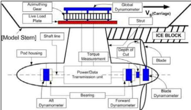
The sketch of an azimuthing model podded propulsor in tractor mode is shown in Figure 1. The propeller design chosen was that for the Canadian Coast Guard Gulf/River Class Medium Icebreaker Ships (R Class propeller). The propeller was scaled to 13.733 and it had a diameter of 0.3 m and four blades. Mean-pitch/diameter ratio (P/D) was 0.76 and expanded blade area ratio (EAR) was 0.669. The diameter of the hub at the propeller was 0.11 m. The blade design was based on the Stone Marine Meridian series (Emerson and Sinclair, 1978), but with thickened blades for operation in ice. The propeller shaft was driven by a 3.3 kW electric drive motor.

The present model had three six-component dynamometers installed to measure blade loads and shaft-bearing loads. The dynamometers were manufactured by Advanced Mechanical Technology Inc. (AMTI) and were capable of measuring forces/moments in six degrees of freedom. They could measure forces up to 2224 N in x- and y- directions, 4448 N in the z- direction, and moments up to 56.5 Nm about all three axes. The AMTI load cell model number for all three dynamometers was MC2.5-6-1000.

Data were sampled at a rate of 5000 Hz, because the propeller rotational speed was high and high frequency data points were needed to monitor the

propeller-ice interaction process. During the course of the experiments, the thickness, flexural, compressive and shear strength values of the ice sheets were sampled at approximately two hourly intervals in order to record the variations in the ice properties. The compressive strengths used for the numerical calculation in this study were 195 kPa and 120 kPa for 35 mm and 15 mm depth of cut respectively. The depth of cut is defined in Figure 2.

Figure 1: Sketch for the model podded propulsor system with measurement devices

Figure 2: Depth of cut and milling angle

3.2 IOT’s ice tank and model ice

The useable area of the tank for ice testing is 76 m long, 12 m wide and 3 m deep. In addition, a 15 m long setup area is separated from the ice sheet by a thermal door to allow equipment preparation while the test sheet is prepared (Figure 3). The range of the carriage speed is from 0.0002 to 4.0 m/s. The carriage is designed with a central testing area where a test frame, mounted to the carriage frame, allows the experimental setup to move transversely across the entire width of the tank. In order to save the ice sheet, the entire ice sheet was pre-cut into three parts; they were called the North Quarter Point, Centre Channel and South Quarter Point. For the ice covered water tests, the Centre Channel was used first, and then the South or North Channel was used with wooden staples to keep the ice sheet in place.

Figure 3: Schematic diagram of the ice tank (after Jones, 1987)

Model EG/AD/S ice was used in these experiments. EG/AD/S ice is specifically designed to provide the scaled flexural strengths of columnar sea ice (Timco, 1986). It is a diluted aqueous solution of ethylene glycol (EG), aliphatic detergent (AD), and sugar (S). The procedure to produce the model ice is as follows. First, the ice sheet is grown by cooling the tank room to approximately -20 oC, then “seeding” the tank by spraying warm water into the cold air in a thin mist, allowing it to form ice crystals before it contacts the surface of the tank. The ice is allowed to grow at approximately -20 oC until it has reached the desired thickness. The temperature of the room is then raised to above freezing and the ice is allowed to warm up and soften, a process called tempering, until the target ice strength is reached. In order to provide uniform properties of the model ice, micro-bubbles for corrected density were not included in the ice, although they are normally used in ship/ice tests.

4.

D

For better understanding of ice loads acting on a propeller, the authors hypothesize that the loads from ice covered water consist of three components: separable hydrodynamic loads, inseparable hydrodynamic loads and ice contact loads. The separable hydrodynamic loads imply loads from open water conditions. During the interaction between a propeller blade and ice, however, as blade hydrodynamic lift will not fully develop when the blade is in the ice or immediately after the blade exits the ice, the separable hydrodynamic loads are only approximate values. The inseparable hydrodynamic loads are mainly generated by a blockage effect, proximity effect, and cavitation due to the presence of ice. The ice milling loads are the contact loads when the blade physically contacts with ice. The inseparable hydrodynamic loads and ice milling loads combined are referred to here as ice related loads and they are defined when the blades are in contact with

ice. This classification helps not only to evaluate accurate ice loads on the blade, but also to develop the ice contact model.

Total Loads in ice (Propeller-Ice Interaction loads) = Ice Milling Loads

+ Separable Hydrodynamic Loads + Inseparable Hydrodynamic Loads

Ice Related Loads = Ice Milling Loads + Inseparable Hydrodynamic Loads

Ice related loads are considered only when the blades are in contact with ice, which is called the milling period. In order to find the appropriate milling period, the milling angle (αm) that corresponded to

the depth of cut was considered (Figure 2 and Table 1).

Table 1: Depth of cut vs. milling angle Depth of cut Milling angle (αm)

15mm 63 degree (10 ~ -53 degrees) 35mm 105 degree (36 ~ -69 degrees) Figure 4 shows an example of the time series data obtained from the experiments. The blade thrust, carriage speed and rps against time are shown. For a time from 48 to 58 seconds, the test condition shows the bollard condition (5 rps and zero carriage speed). In the tractor mode, the propeller rotated counter-clockwise, thus the rps was shown as a negative value.

Figure 4: Time series data for blade thrust vs. rps & carriage speed

If Figure 4 is expanded, for example at the 65th second segment, then the enlarged segment is given in Figure 5. In the graph shown in Figure 5, the separable hydrodynamic loads have already been removed and the ice-related loads are shown by open

triangles. The separable hydrodynamic loads were the values measured in the open water tests. The figure shows that the blade enters the ice block at the blade angular position of 36 degrees and exits at negative 69 degrees. This period was defined as the milling period. Time (sec) Bl a d e th ru st (N ) B la de a ng ul a r p o si ti o n (de g ) 65 65.1 65.2 65.3 65.4 65.5 -100 -50 0 50 100 150 200 250 300 -200 -150 -100 -50 0 50 100 150 200 Blade thrust

Blade thrust (During milling of the ice) Blade angular position

Key blade starts to enter the ice block

36 deg

Key blade starts to exit the ice block

-69 deg 36 deg

-69 deg

Figure 5: Blade thrust during the milling period based on the milling angle (α : from 36 degrees to -69 _m

degrees, 35mm depth of cut and 5 rps)

It is noted that the blade angular position was measured up to positive and negative 180 degrees. From approximately - 160 degrees to - 180 degrees, the blade angular positions could not be measured because of limitations of the sensor.

5.

N

P

5.1 Overview of numerical code (PROPICE)

The code used in this study was originally developed at the NASA Ames, and was called PMARC. Bose (1996) modified this code for propeller performance in blocked flow. This modified code was called PROPS. In this study, the PROPS code was used as the basic frame and some parts were modified and developed to include the ice milling loads calculations; this modified code was called PROPICE. In the PROPICE code, the propeller blades only were modeled by using 44 chordwise and 18 spanwise panels, as shown in Figure 6.

Figure 6: Geometry and paneling of the propeller For separable hydrodynamic loads, a procedure for typical panel method is used without any ice consideration. When the blade contacts with ice, however, the process for the ice related loads calculation is activated. The panels of the blade within the ice block experience either inseparable hydrodynamic loads or ice milling loads and they should be identified; detailed procedure is addressed in the next section. Generally, the inseparable hydrodynamic loads are generated due to the presence of ice without any physical contact; for example, blockage, proximity and cavitation. In this study, however, only a simplified blockage condition was considered.

For the numerical calculation in blocked flow, a simplified ice wake model was used in this study. The ice block itself did not need to be modeled physically in the code, but it was considered conceptually. For the blockage model, it was assumed that the propeller was rotating in a simplified wake behind the ice; the simplified ice wake was defined such that the downstream velocity in the wake of the block was 0.01 times that of the free stream (similarly to that done by Bose, 1996).

5.2 Numerical procedure for ice related loads

When the propeller blades contact with the ice, the subroutine for the ice related load calculations is activated and the ice related loads are calculated at the blade panels which are in contact with ice. The compressive strength of the model ice measured during the experiments is taken into account as the ice reference pressure for the numerical calculation. The procedure of the ice related loads calculation is addressed below.

[Step.1] Determination of a depth of cut, an ice reference pressure ( ) and an azimuthing angle (

) ( ICE REF

P

ψ ) of the system as input data. In order to provide the uniform interaction conditions between the propeller and ice, the calculations were performed in the tractor mode only; for the pusher mode, the pod and strut interact with the ice block before the propeller, so ice blocks can be disturbed. The azimuthing angles used in this calculation are 180, 150, 120 and 90 degrees in the tractor mode. Two different depths of cut, 15 and 35 mm, were considered. The ice reference pressure of the calculation for the 15 mm and 35 mm depths of cut were 120 kPa and 195 kPa, respectively.

[Step.2] Determination of the panels which are in contact with the ice block. Once the coordinate of the bottom of the conceptual ice block is defined, the blade panels can be identified with their radial components; if the radial component of the blade is larger than the bottom line of the conceptual ice block, then the panel is assumed to be in contact with the ice block. The positive direction of the radial component of the blade is from the root to the tip of the blade.

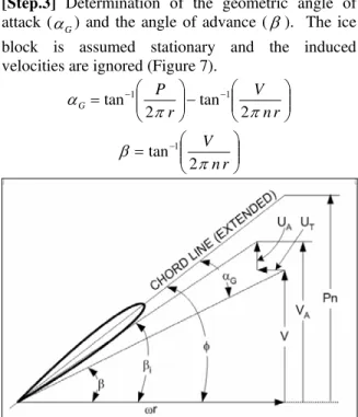
[Step.3] Determination of the geometric angle of attack (α ) and the angle of advance (_G β). The ice block is assumed stationary and the induced velocities are ignored (Figure 7).

⎟⎟ ⎠ ⎞ ⎜⎜ ⎝ ⎛ − ⎟⎟ ⎠ ⎞ ⎜⎜ ⎝ ⎛ = − − r n V r P G _{π π} α 2 tan 2 tan 1 1 ⎟⎟ ⎠ ⎞ ⎜⎜ ⎝ ⎛ = − r n V π β 2 tan 1

Figure 7: Velocity diagram for a propeller blade section, βis the angle of advance, β is the _i hydrodynamic pitch angle, φ is the geometric pitch

angle, α is the geometric angle of attack, V is the _G carriage speed, is the advance speed, and

are the tangential and axial induced velocities, and A V U_T A U Pis the pitch at 0.7R

[Step.4] Choice between the milling and blockage area at each panel which contacts with ice. Depending on the angle of advance, panels can be identified as either the milling or blockage area (including shadowing), as shown in Figure 8. If the interacting angle (Θ ), which is the angle between the normal vector of the panel and the directional vector of the angle of advance, is greater than 0 degrees and less than 90 degrees, then this panel is involved in the milling area; if this interacting angle ( ) is more than 90 degrees or less than 0 degrees, then this panel is involved in the blockage area.

Θ

Figure 8: Geometrical consideration for the ice contact area (Θ : the interacting angle)

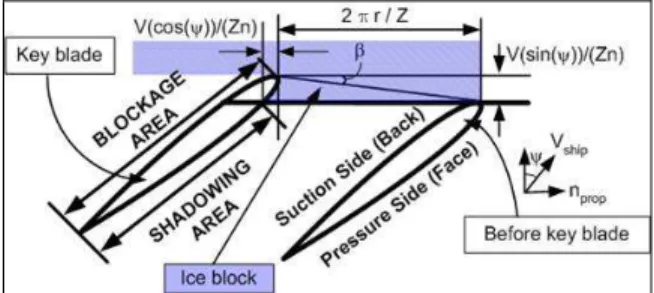
[Step.5] Correction of the shadowing area. Once the panel is identified as the milling area, the shadowing area should be checked. If the panel is within the shadowing area, then the panel must be considered as blockage area. When a certain azimuthing angle, which is less than 180 degrees and more than 90 degrees, is given, additional kinematic considerations are made, as shown in Figure 9. Once the shadowing area is determined, the calculation is performed in the same manner as the blockage area.

The principle to calculate the shadowing area is: 1. Relative motion between the propeller and

carriage (ship) is taken into account with two directions, which are axial (perpendicular to the propeller rotating direction) and propeller rotating directions (n =n_PROP);

2. The advance distance at each blade is to be

n Z

V

V(= ship) _{based on the angle of advance}

(β);

3. Once the azimuthing angle is less than 180 degrees (tractor mode), contribution of the azimuthing angle (ψ ) on the axial and rotational direction must be considered; i.e. the advance and rotational distances are n Z Vsin(ψ) _and n Z Vcos(ψ)_{, respectively;} 4. If the panels are placed out of the advance

or rotational distances then the panels are finally identified as the shadowing area, even though the panels belong to the milling area, as shown in [Step.4]

Figure 9: Shadowing area at various azimuthing angles

[Step.6] Determination of the pressure coefficient at each panel. The total pressure coefficient ( ) is sum of the hydrodynamic pressure and ice crushing pressure coefficients, as shown in below:

) (TOTAL P C ) ( ) ( )

(TOTAL PHYDRODYNAMIC PCRUSHING

P C C

C = +

The hydrodynamic pressure values can be calculated by using the panel method and the ice crushing pressure coefficient can be evaluated by empirical formulae based on geometric and kinematic considerations. If the interacting angle (Θ ) is 0 degrees, then the panel interacts with the ice perpendicularly, which is called pure crushing. On the other hand, if the interacting angle (Θ ) is 90 degrees, then the panel interacts with the ice in parallel, which is called pure shearing. The crushing pressure is calculated based upon the ice reference pressure and the interacting angle (Θ ). An empirical factor for crushing (EFC) was introduced and this was multiplied by the ice reference pressure. A value of EFC equal to 7 was used to empirically represent the effect of high strain rate failure of ice. It is assumed that the crushing pressure is distributed

using a cosine distribution relative to the interacting angle (Θ ). The ice crushing pressure coefficient can then be calculated from

(

)

where P_{REF( ICE)}is the ice reference pressure, Θ is the interacting angle, ρ_I is the ice density, W is the weight factor, EFC is the empirical factor for crushing, and is the local inflow velocity (inflow velocity (V ) + propeller rotational velocity (

ref

V

r

× Ω )). Shearing forces were considered independently, because they cannot be represented in the pressure term. Constant shearing forces were applied to the milling area. These were the ice reference pressure divided by an empirical factor for shearing (EFS), which was taken as equal to two. From the ice samplings during the tests, the compressive strength was found to be two to four times the shear strength. Below equation shows the shearing force:

AREA EFS P F REFICE SHEARING = × ) ( ) (

where EFS is the empirical factor for shearing and is the area of the panel.

AREA

The discussions of these empirical factors were presented in Wang et al. (2008). It is noted that the frictional force in ice is not considered because the shearing force can include the friction; the ice frictional coefficient is as small as 0.02 (Gagnon and Molgaard, 1991).

[Step.7] Calculation of the total forces from the hydrodynamic loads and the ice related loads. Thrust and torque coefficients are calculated from the total forces.

It is noted that these empirical factors are used for blade loads only. We experienced that there were discrepancy between shaft loads and blade loads possibly because of shaft dynamics.

6.

C

The experimental results measured from the blade dynamometer were compared with numerical results for which only the key blade loads were calculated. For the experiments, maximum and average values were picked during each milling period, and then their mean values were calculated. For the numerical values, only the milling period was considered; i.e.,

all values were set to zero except those in the milling period. The maximum and average values from PROPICE were picked from the last cycle (third cycle) only. In this paper only blade loads at the azimuthing angle of 180 degrees in tractor mode are presented.

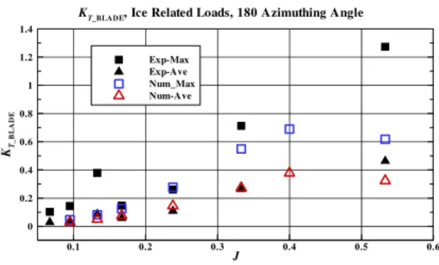
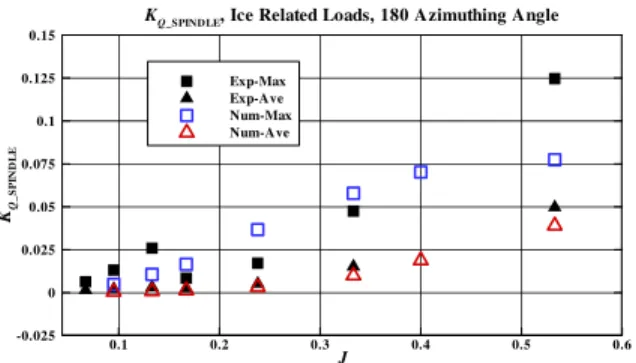
From Figure 10 to Figure 13, the coefficients of blade thrust, blade torque, out of plane bending moment and spindle torque against the advance coefficient are presented. The test conditions are: tractor mode, an azimuthing angle of 180 degrees, and a 35 mm depth of cut. The solid symbols represent experimental results, and the open symbols represent numerical results.

The trends of the blade thrust are described here. From the numerical calculations, the shadowing effect occurred at the lower advance coefficient (J < 0.4). For example, at the advance coefficient of 0.1, approximately 23 % of the pressure side panels of the blade within the ice block experience ice contact loads due to the shadowing effect (Wang, 2007; Wang et al., 2008). As the advance coefficient increases to 0.4, the thrust coefficients show the increased trends. This is caused by the combined effect of the angle of attack and shadowing. Generally, as the angle of attack is decreased, the thrust coefficients decrease; as the shadowing effect is decreased, the thrust coefficients increase. When the advance coefficient is 0.4, the shadowing effect is almost negligible. As the advance coefficient increases over 0.4, the angle of attack decreases, thus the thrust coefficient starts to decrease.

In the figures, the numerical results for both average and maximum are relatively well predicted, particularly at the lower advance coefficients (J < 0.4). As the advance coefficients increase to value over 0.4, estimated values of thrust, torque, out of plane bending moment and spindle torque are different from experimental values. This may be explained by the variation of the depth of cut. As the model stern of the podded propulsor slightly pushes down on the ice sheet, depths of cut may be changed due to the inertia of the ice sheet, especially at the high carriage velocities. It was also found that ice pieces sometimes accumulated in front of the model stern, thus the depth of cut could be changed.

J KT _ B L ADE 0.1 0.2 0.3 0.4 0.5 0 0 0.2 0.4 0.6 0.8 1 1.2 1.4 .6 Exp-Max Exp-Ave Num_Max Num-Ave

KT_BLADE, Ice Related Loads, 180 Azimuthing Angle

Figure 10: KT_BLADE comparison (ice related loads,

azimuthing angle of 180 degrees, 35 mm depth of cut, key blade only)

J KQ _ B L ADE 0.1 0.2 0.3 0.4 0.5 0.6 -0.1 0 0.1 0.2 0.3 0.4 0.5 0.6 0.7 0.8 Exp-Max Exp-Ave Num-Max Num_Ave

K_{Q_BLADE}, Ice Related Loads, 180 Azimuthing Angle

Figure 11: KQ_BLADE comparison (ice related loads,

azimuthing angle of 180 degrees, 35 mm depth of cut, key blade only)

J KM _ OOP 0.1 0.2 0.3 0.4 0.5 0.6 -1 -0.9 -0.8 -0.7 -0.6 -0.5 -0.4 -0.3 -0.2 -0.1 0 0.1 Exp-Max Exp-Ave Num-Max Num-Ave

KM_OOP, Ice Related Loads, 180 Azimuthing Angle

Figure 12: KM_OPLANE comparison (ice related loads,

azimuthing angle of 180 degrees, 35 mm depth of cut, key blade only)

J KQ _ S P INDL E 0.1 0.2 0.3 0.4 0.5 0.6 -0.025 0 0.025 0.05 0.075 0.1 0.125 0.15 Exp-Max Exp-Ave Num-Max Num-Ave

KQ_SPINDLE, Ice Related Loads, 180 Azimuthing Angle

Figure 13: KQ_SPINDLE comparison (ice related loads,

azimuthing angle of 180 degrees, 35 mm depth of cut, key blade only)

7.

C

Model tests for propeller-ice interaction were carried out in the ice tank and the test results were presented. An azimuthing podded propulsor model allowed to examine the propeller ice interaction loads with various thrust directions. For a tractor mode, steady milling condition can be assumed and detailed interaction phenomena were observed. Based on this condition, empirical model for ice loads was developed and implemented into panel code. The comparison between experiments and numerical calculations shows good agreement.

7.1 Propeller performance in ice

From this study, it is found that there are a few key parameters to affect propeller performance during propeller-ice interaction; propeller rps, ship speed, pitch angle, depth of cut, and ice property (compressive strength possibly). Based on these parameters, three major terms to affect propeller performance were suggested; angle of attack, advance coefficient and shadowing effect -these three terms are a function of above five parameters. It is concluded that there are three periods to change propeller performance for a 35 mm depth of cut at 180°azimuthing angle:

z _{First stage at low advance coefficient (0 < J <} 0.4): Thrust increases because the shadowing area starts to decrease and the ice milling area on pressure side increases due to the increase in the angle of advance z Second stage at intermediate advance

coefficient (0.4 < J < 0.7): Thrust decreases because the ice milling area on suction side increases and ice milling loads on the pressure side decrease

z Third stage at high advance coefficient ( J > 0.7): Thrust decreases because the milling area on the suction side increases and the milling area on the pressure side almost disappears

R

[1] Akinturk, A., Jones, S.J., Duffy, D. and Rowell, B., 2004a. Ice Loads on Azimuthing Podded Propulsors. Proc. 23rd International Conference on Offshore Mechanics and Arctic Engineering, (OMAE’04), June 20-25, New York.

[2] Akinturk, A., Jones, S., Duffy, D., and Rowell, B., 2004b. Measuring Podded Propulsor Performance in Ice. Proceedings of the 1st International Conference on Technological Advances in Podded Propulsion, School of Marine Science and Technology, University of Newcastle Upon Tyne, UK, pp. 187-198.

[3] Bose, N., 1996. Ice Blocked Propeller Performance Prediction Using a Panel Method. Trans. Royal Institution of Naval Architects, 138, pp.213-226.

[4] Emerson, A. and Sinclair, L., 1978. Propeller Design and Model Experiments. Trans. North East Coast Institution of Engineers and Shipbuilders, 94, pp. 199-234 and D31-34.

[5] Gagnon, R. and Molgaard, J., 1991. Crushing Friction Experiments on Freshwater Ice. Proc. IUTAM-IAHR Symposium, S. J. Jones et al., ed., Springer, Berlin, pp.405-421.

[6] Jones, S. J., 1987. Ice Tank Test Procedure at the Institute for Marine Dynamics. Report No. LM-AVR-20, Institute for Ocean Technology, National Research Council of Canada.

[7] Jones, S. J., Soininen, H., Jussila, M., Koskinen, P., Newbury, S. and Browne, R., 1997. Propeller-Ice Interaction. Trans. Society of Naval Architects and Marine Engineers, 105, pp. 399-425.

[8] Mintchev, D., Bose, N., Veitch, B., Atlar, M. and Paterson, I., 2001. Some Analysis of Propeller Ice Milling Experiments. Proc. 6th Canadian Marine Hydromechanics and Structures Conference '01, Vancouver, BC, Canada.

[9] Moores, C., Veitch, B., Bose, N., Jones, S. J. and Carlton, J., 2002. Multi-Component Blade Load Measurements on a Propeller in Ice. Trans. Society of Naval Architects and Marine Engineers, 110, pp. 169-188.

[10] Searle, S., Veitch, B. and Bose, N., 1999. Ice-Class Propeller Performance in Extreme Conditions. Trans. Society of Naval Architects and Marine Engineers, 107, pp. 127-152.

[11] Soininen, H., 1998. A Propeller-Ice Contact Model. Dissertation for the degree of Doctor of Technology, Helsinki University of Technology, Espoo.

[12] Timco, G., 1986. EG/AD/S: A New Type of Model Ice for Refrigerated Towing Tanks. Cold Regions Science and Technology, 12, pp. 175-195. [13]Varma, G., 2000. Ice Loads on Propellers under Extreme Operating Conditions. Master Thesis, Memorial University of Newfoundland, Canada. [14] Veitch, B., 1995. Predictions of Ice Contact Forces on a Marine Screw Propeller during the Propeller-Ice Cutting Process. Acta Polytechnica Scandinavica, Mechanical Engineering Series, Helsinki, 118.

[15] Wang, J., 2007. Prediction of Propeller Performance on a Model Podded Propulsor in Ice (Propeller-Ice Interaction). Ph.D. Thesis, Memorial University of Newfoundland, Canada.

[16] Wang, J., Akinturk, A., Foster, W., Jones, S. J. and Bose, N., 2004. An Experimental Model for Ice Performance of Podded Propellers. Proc. 27th American Towing Tank Conference, Institute for Ocean Technology, National Research Council of Canada.

[17] Wang, J., Akinturk, A., Jones, S. J. and Bose, N., 2005. Ice Loads on a Model Podded Propeller Blade in Milling Conditions. Proc. 24th International Conference on Offshore Mechanics and Arctic Engineering, (OMAE’05), Halkidiki, Greece.

[18] Wang, J., Akinturk, A. and Bose, N., 2006. Numerical Prediction of Model Podded Propeller-Ice Interaction Loads. Proc. 25th International Conference on Offshore Mechanics and Arctic Engineering, Hamburg, Germany.

[19] Wang, J., Akinturk, A., Jones, S. J., Bose, N., Kim, M.C., and Chun, H.H., 2007. Ice Loads Acting on a Model Podded Propeller Blade. ASME J. Offshore Mechanics and Arctic Engineering, 129(3). [20] Wang, J., Akinturk, A., and Bose, N., 2008. Numerical Prediction of Propeller Performance during Propeller Ice Interaction, Marine Technology, paper was submitted.