HAL Id: hal-02069222
https://hal.archives-ouvertes.fr/hal-02069222
Submitted on 15 Mar 2019
HAL is a multi-disciplinary open access
archive for the deposit and dissemination of
sci-entific research documents, whether they are
pub-lished or not. The documents may come from
teaching and research institutions in France or
abroad, or from public or private research centers.
L’archive ouverte pluridisciplinaire HAL, est
destinée au dépôt et à la diffusion de documents
scientifiques de niveau recherche, publiés ou non,
émanant des établissements d’enseignement et de
recherche français ou étrangers, des laboratoires
publics ou privés.
airGR and airGRteaching: Two Open-Source Tools for
Rainfall-Runoff Modeling and Teaching Hydrology
Olivier Delaigue, G. Thirel, L. Coron, P. Brigode
To cite this version:
Olivier Delaigue, G. Thirel, L. Coron, P. Brigode. airGR and airGRteaching: Two Open-Source Tools
for Rainfall-Runoff Modeling and Teaching Hydrology. 13th International Conference on
Hydroinfor-matics (HIC 2018), Jul 2018, Palerme, Italy. pp.541-548. �hal-02069222�
airGR and airGRteaching: two open source
tools for rainfall-runoff modeling and teaching
hydrology
Olivier Delaigue
1, Guillaume Thirel
1, Laurent Coron
1,2, Pierre Brigode
31
Irstea, HYCAR, Hydrology Research Group, Antony, France 2 Now at: EDF DTG, Toulouse, France
3 Université Côte d'Azur, CNRS, OCA, IRD, Géoazur, Nice, France [email protected], [email protected]
Abstract
In this paper, we present two R packages, airGR and airGRteaching, which are aimed at hydrological modeling. These two open-source packages allow for undertaking simplified simulations of surface flows on river catchments, based on lumped rainfall-runoff models that require few input data. airGR can be used for engineering, research and education purposes and is well indicated for experiments on large sample datasets. airGRteaching is an add-on to airGR and is especially dedicated to education, since one of its functionalities provides an interface on which parameters and models fluxes can be easily understood through an interactive visualization. airGRteaching also contains simplified functions that require less programming from users but do not allow for some more advanced experiments.
1 Introduction
Lumped hydrological models are useful and convenient tools for research, engineering and educational purposes. They propose catchment-scale representations of the precipitation-discharge relationship. Thanks to their limited data requirements, they can easily be implemented and run. With such models, it is possible to simulate a number of hydrological key processes over the catchments with limited structural and parametric complexity, typically evapotranspiration, runoff and underground losses. The Hydrology Group at Irstea (Antony) has been developing a suite of rainfall-runoff models (i.e. catchment scale representations of the precipitation discharge relationship) over the past 30 years with the main objectives of designing models as efficient as possible in terms of streamflow simulation, applicable to a wide range of catchments and having low data requirements. This resulted in a suite of models running at different time steps (from hourly to annual) applicable
Engineering
Volume 3, 2018, Pages 541–548
HIC 2018. 13th International Conference on Hydroinformatics
for various issues including water balance estimation, forecasting, simulation of impacts and scenario testing.
Recently, Irstea has developed an easy-to-use R package (Coron et al., Environmental Modelling & Software, 2016; Coron et al., R package version 1.0.9.64, 2017), called airGR, to make these models widely available and facilitates reproducible science. It is available on the Comprehensive R Archive Network (CRAN)* and it includes several hydrological models. In addition, a further R package, airGRteaching (Delaigue et al., R package version 0.2.2.2, 2018), has been developed to ease the use of airGR, especially through a graphical interface. This communication aims at presenting these two R packages.
2 Material
2.1 airGR
The airGR package includes hydrological models functioning at several time steps (from hourly to annual) and a snow accumulation and melt model. All these models were developed with a common philosophy: the models must be parsimonious in terms of required input data and parameters to calibrate, and they must include only the necessary process to accurately represent the rainfall-runoff relationship. Several models developed at Irstea since the 1990s are available in airGR, namely:
• the water balance annual GR1A (Mouelhi et al., Journal of Hydrology, 2006) model, • the monthly GR2M (Mouelhi, PhD thesis, 2003) model,
• three versions of the daily model, namely GR4J (Perrin et al., Journal of Hydrology, 2003), GR5J (Le Moine, PhD thesis, 2008) and GR6J (Pushpalatha et al., Journal of Hydrology, 2011),
• the hourly GR4H model (Mathevet, PhD thesis, 2005),
• a degree-day snow model CemaNeige (Valéry et al., Journal of Hydrology, 2014).
Applications of the listed models can thus encompass numerous topics, for example water balance and water resources assessment, catchments regimes estimation, climate change impact application, fast responding or snow-fed catchments, hydrological forecasting. The airGR package has been designed to facilitate the use by non-expert users and to allow users to customize their own additional evaluation criteria, models or calibration algorithm. A tutorial† and an included documentation of all functions that are written in English are available. The in-built airGR calibration algorithm is based on a pre-screening of the parameters space followed by a steepest gradient method. Specific vignettes describing how to use local or global calibration algorithms that are provided in other R packages are included in airGR since version 1.9.0.64.
Each hydrological model core and the snow model core are coded in FORTRAN to ensure fast computation. The other package functions (i.e. mainly the calibration algorithm, a routine calculating potential evapotranspiration based on the Oudin formula (Oudin et al., Journal of Hydrology, 2005) and the efficiency criteria) are coded in R, which ensures a great flexibility of computer programming. It allows for convenient implementation of model inter-comparisons and large sample hydrology experiments.
2.2 airGRteaching
airGR is used for educational purposes at universities or engineering schools. In order to avoid the difficulties that students may have with R programming or when manipulating datasets, the
*https://cran.r-project.org/ †
https://webgr.irstea.fr/airGR-website
airGR and airGRteaching: Two Open-source Tools for Rainfall-Runoff Modeling ... O. Delaigue et al.
airGRteaching R package (Delaigue et al., R package version 0.2.2.2, 2018) was recently developed. It includes the following features:
• three simplified functions to prepare data, calibrate a model and run a simulation, • additional static and dynamic plot functions,
• a function that launches a graphical user interface connecting R to a Web browser.
The simplified functions are proposed in order to help students not to be confused with the large number of arguments of the original functions. Some functions allow for producing static charts that can be used by students for reporting. Other functions generate HTML5/Javascript dynamic charts that are useful tools to identify data issues and to explore into more details particular periods by click-and-drag zooming on the graphs.
3 Results
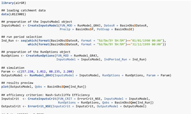
Due to its simplicity and the possibility to modify crucial arguments, such as the studied period, parameters or model names (Figure 1), and because the CPU time required for running the models is very low (from less than one second for any year simulation up to less than a minute for any 10-year calibration, see Tab. B3 in (Coron et al., Environmental Modelling & Software, 2016)), airGR allows for making systematic tests on large sample of catchments. airGR has already been applied in the context of model intercomparisons (de Boer-Euser et al., Hydrology and Earth System Sciences, 2017), model applications (Crochemore, PhD thesis, 2016), model improvements (Ficchí, PhD thesis, 2017) and is used by consultants and water engineers.
library(airGR)
## loading catchment data data(L0123001)
## preparation of the InputsModel object
InputsModel <- CreateInputsModel(FUN_MOD = RunModel_GR4J, DatesR = BasinObs$DatesR, Precip = BasinObs$P, PotEvap = BasinObs$E)
## run period selection
Ind_Run <- seq(which(format(BasinObs$DatesR, format = "%d/%m/%Y %H:%M")=="01/01/1990 00:00"), which(format(BasinObs$DatesR, format = "%d/%m/%Y %H:%M")=="31/12/1999 00:00"))
## preparation of the RunOptions object
RunOptions <- CreateRunOptions(FUN_MOD = RunModel_GR4J,
InputsModel = InputsModel, IndPeriod_Run = Ind_Run) ## simulation
Param <- c(257.238, 1.012, 88.235, 2.208)
OutputsModel <- RunModel_GR4J(InputsModel = InputsModel, RunOptions = RunOptions, Param = Param)
## results preview
plot(OutputsModel, Qobs = BasinObs$Qmm[Ind_Run])
## efficiency criterion: Nash-Sutcliffe Efficiency
InputsCrit <- CreateInputsCrit(FUN_CRIT = ErrorCrit_NSE, InputsModel = InputsModel, RunOptions = RunOptions, Qobs = BasinObs$Qmm[Ind_Run]) OutputsCrit <- ErrorCrit_NSE(InputsCrit = InputsCrit, OutputsModel = OutputsModel)
## Crit. NSE[Q] = 0.7985
In Figure 1, the main steps needed for running a hydrological model with airGR are given. First, data (precipitation, temperature and / or potential evapotranspiration) must be loaded and prepared at the required format. Then, the run options (model name, period of simulation) must be defined. In order to be run, parameters must be defined, either through automatic calibration (not shown here) or manually (as shown here). Finally, the results can be plotted and analysed with the use of existing criteria formulas. It is obvious that the use of a loop on a list of catchments of interest or on a list of periods will automatize the obtaining of results with very limited additional coding.
Three simplified functions exist in airGRteaching, namely to prepare data, calibrate a model and run a simulation. In Figure 2, the use of the functions to prepare data and to calibrate the GR4J model with CemaNeige is shown. As can be easily inferred from the comparison of Figure 1 and Figure 2, the code is much simplified in airGRteaching. However, some basic features that are often required for more advanced tests are not available in airGRteaching (e.g. defining the initial states, fixing some of the parameters when an automatic calibration is performed and allowing for calibration on discontinuous periods). Furthermore, if one wants to calculate several performance criteria, it is necessary to run the model several times in airGRteaching whereas in airGR only one run is necessary as the outputs can be used as an input of a criterion calculation function.
library(airGRteaching)
## data.frame of observed data data(L0123001)
BasinObs2 <- BasinObs[, c("DatesR", "P", "E", "Qmm", "T")]
## Preparation of observed data for modelling
PREP <- PrepGR(ObsDF = BasinObs2, HydroModel = "GR4J", CemaNeige = TRUE)
## Calibration step
CAL <- CalGR(PrepGR = PREP, CalCrit = "KGE2",
WupPer = NULL, CalPer = c("1990-01-01", "1993-12-31"))
## Grid-Screening in progress (0% 20% 40% 60% 80% 100%) ## Screening completed (729 runs)
## Param = 169.017 , -0.020 , 83.096 , 2.384 , 0.002 , 6.764 ## Crit KGE'[Q] = 0.8773
## Steepest-descent local search in progress ## Calibration completed (19 iterations, 936 runs)
## Param = 157.591 , 0.476 , 83.096 , 2.198 , 0.002 , 6.000 ## Crit KGE'[Q] = 0.9115
plot(CAL, which = "iter")
Figure 2: Example of the code used for preparing observed data and for calibrating GR4J in airGRteaching.
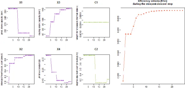
The Figure 3 shows the output of the plot function used on Figure 2 on the calibration object. Here, the evolution of the model parameters and performance for each improvement of the objective function are shown for the steepest gradient step of the automatic calibration algorithm.
airGR and airGRteaching: Two Open-source Tools for Rainfall-Runoff Modeling ... O. Delaigue et al.
Figure 3: Output of the airGRteaching plot function with a calibration object. The evolution of the four GR4J parameters and of the two CemaNeige parameters as well as of the objective function during the steepest gradient process are given.
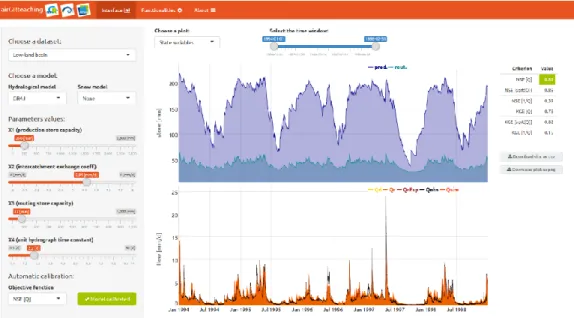
The airGRteaching graphical user interface is presented on Figure 4. It is based on the Shiny (Chang et al., R package version 1.1.0, 2018) R package. On the left is presented the sidebar panel, which allows to select the basin studied (the interface is launched with data that have been previously loaded in the R environment) and the model used (only daily models are available in the interface) and also to modify the model parameters with a slider widget. At the bottom of this sidebar, a button allows to automatically calibrate the model. At the center, the tab pan allows to show four reactive plots that show:
• the precipitations and flows time series,
• a set of synthetic plots to evaluate the model performance, • the time series of internal variables (Figure 5),
• input and outputs time series and the model scheme (Figure 4), on which the model fluxes vary over time (if the animation is activated).
On the right side, there is a radio button to overlap on the time series plots the previous flow simulation in order to compare it with the current simulation and better understand the role of the changed parameter(s). In addition, a table presents different efficiency criteria values relative to the current (and previous) simulation. The graphics and the model outputs can be export respectively in the PNG and the CSV formats.
Figure 4: Overview of one of the airGRteaching interface panels.
Figure 5: Overview of the airGRteaching interface panel that shows the evolution of internal model stores (top) and the two components of discharge in GR4J (bottom).
4 Conclusions
airGR is available on the CRAN since beginning of 2017 and is continuously upgraded with additional features issued from the development works lead at Irstea. Future additions to airGR could be a newly developed interception store in GR4H (Ficchí, PhD thesis, 2017), the possibility to use airGR and airGRteaching: Two Open-source Tools for Rainfall-Runoff Modeling ... O. Delaigue et al.
GR4H at finer time steps for fast-responding catchments (Ficchí, PhD thesis, 2017) or an improved snow model that could make use of satellite snow cover area data(Riboust et al., Journal of Hydrology and Hydrodynamics, 2019). This package is already used worldwide in more than 40 countries on all continents, by universities, state services, engineering firms, insurers (Figure 6) and was downloaded more than 5400 times on the CRAN (as of 27 February 2018). airGRteaching will be soon publicly available on the CRAN. It has already been tested in several French universities and engineering schools (Roux and Brigode, Geophysical Research Abstracts, 2018). Additional visualization of the CemaNeige snow model will be implemented in the future in the airGRteaching Shiny interface. It is also planned to allow the use of annual, monthly and hourly models (GR1A, GR2M and GR4H) in this interface.
Figure 6: Countries in which users downloaded airGR. Data up to January 2017 (CRAN downloading do not provide the origin of downloads).
References
Chang, W., Cheng, J., Allaire, JJ., Xie, Y. and McPherson, J. (2018). shiny: Web Application Framework for R. R package version 1.1.0. https://CRAN.R-project.org/package=shiny Coron, L., Thirel, G., Delaigue, O., Perrin, C. and Andréassian, V. (2017). The Suite of Lumped GR
Hydrological Models in an R package, Environmental Modelling & Software, 94, 166-171, DOI: 10.1016/j.envsoft.2017.05.002
Coron, L., Perrin, C., Delaigue, O., Thirel, G. and Michel, C. (2017). airGR: Suite of GR Hydrological Models for Precipitation-Runoff Modelling. R package version 1.0.9.64. URL: https://webgr.irstea.fr/en/airGR/
Crochemore, L. (2016). Seasonal streamflow forecasting for reservoir management. PhD thesis, Irstea (Antony), AgroParisTech (Paris), 213 pp.
Delaigue, O., Coron, L. and Brigode, P. (2018). airGRteaching: Tools to Simplify the Use of the airGR Hydrological Package for Education (Including a Shiny Interface). R package version
de Boer-Euser, T., Bouaziz, L., De Niel, J., Brauer, C., Dewals, B., Drogue, G., Fenicia, F., Grelier, B., Nossent, J., Pereira, F., Savenije, H., Thirel, G., and Willems, P. (2017). Looking beyond general metrics for model comparison – lessons from an international model intercomparison study, Hydrology and Earth System Sciences, 21, 423-440, DOI: 10.5194/hess-21-423-2017. Ficchí, A. (2017). An adaptive hydrological model for multiple time-steps: Diagnostics and
improvements based on fluxes consistency. PhD thesis, Irstea (Antony), GRNE (Paris), 281 pp.
Le Moine, N. (2008). Le bassin versant de surface vu par le souterrain : une voie d’amélioration des performances et du réalisme des modèles pluie-débit ? PhD thesis, Université Pierre et Marie Curie (Paris), Cemagref (Antony), 324 pp.
Mathevet, T. (2005). Quels modèles pluie-débit globaux pour le pas de temps horaire ? Développement empirique et comparaison de modèles sur un large échantillon de bassins versants. PhD thesis, ENGREF (Paris), Cemagref (Antony), France, 463 pp.
Mouelhi S. (2003). Vers une chaîne cohérente de modèles pluie-débit conceptuels globaux aux pas de temps pluriannuel, annuel, mensuel et journalier. PhD thesis, ENGREF, Cemagref Antony, France, 323 pp.
Mouelhi, S., Michel, C., Perrin, C. and Andréassian, V. (2006). Stepwise development of a two-parameter monthly water balance model. Journal of Hydrology, 318(1-4), 200-214, DOI: 10.1016/j.jhydrol.2005.06.014.
Oudin, L., Hervieu, F., Michel, C., Perrin, C., Andréassian, V., Anctil, F. and Loumagne, C., 2005. Which potential evapotranspiration input for a rainfall-runoff model? Part 2 – Towards a simple and efficient PE model for rainfall-runoff modelling. Journal of Hydrology, 303(1-4), 290-306, DOI: 10.1016/j.jhydrol.2004.08.026.
Perrin, C., Michel, C. and Andréassian, V. (2003). Improvement of a parsimonious model for streamflow simulation. Journal of Hydrology, 279, 275-289, DOI: 10.1016/S0022-1694(03)00225-7.
Pushpalatha, R., Perrin, C., Le Moine, N., Mathevet, T. and Andréassian, V. (2011). A downward structural sensitivity analysis of hydrological models to improve low-flow simulation.
Journal of Hydrology, 411(1-2), 66-76, DOI: 10.1016/j.jhydrol.2011.09.034.
Riboust, P., Thirel, G., Le Moine, N., and Ribstein, P. (2019). Revisiting a simple degree-day model for integrating satellite data: implementation of SWE-SCA hystereses. Journal of Hydrology
and Hydrodynamics, 67, DOI: 10.2478/johh-2018-0004, accepted.
Roux, Q. and Brigode, P. How long would we have to wait before (re)filling the Malpasset dam reservoir? An example of a teaching project done using R and airGR modeling packages.
Geophysical Research Abstracts, Vol. 20, EGU2018-4108-2, 2018, EGU General Assembly
2018.
Valéry, A., Andréassian, V. and Perrin, C. (2014). ‘As simple as possible but not simpler’: What is useful in a temperature-based snow-accounting routine? Part 2 – Sensitivity analysis of the Cemaneige snow accounting routine on 380 catchments, Journal of Hydrology, 517(0), 1176-1187, DOI: 10.1016/j.jhydrol.2014.04.058.
airGR and airGRteaching: Two Open-source Tools for Rainfall-Runoff Modeling ... O. Delaigue et al.