Charge separation associated with frost growth

CHARGE SEPARATION ASSOCIATED WITH FROST GROWTH by

JAMES PETER RYDOCK

S. B., Physics

Massachusetts Institute of Technology

(1985)

SUBMITTED TO THE DEPARTMENT OF EARTH, ATMOSPHERIC, AND PLANETARY SCIENCES IN PARTIAL FULFILLMENT OF THE REQUIREMENTS FOR

THE DEGREE OF

MASTER OF SCIENCE IN METEOROLOGY at the

MASSACHUSETTS INSTITUTE OF TECHNOLOGY February 1989

@ Massachusetts Institute of Technology

Signature of Author

Department of Earth, Atmospheric, and Planetary Sciences November 3, 1988 Certified by Earle R. Williams Thesis supervisor Accepted by_...__________________ Thomas H. Jordan Department Chairman

ITHDPWVo"

FRO1

MIT

LB

P

CHARGE SEPARATION ASSOCIATED WITH FROST GROWTH by

JAMES PETER RYDOCK

Submitted to the Department of Earth, Atmospheric, and Planetary Sciences on November 3, 1988 in partial fulfillment of the requirements for the Degree of

Master of Science in Meteorology ABSTRACT

Measurements are made of the electrical charge transfer from cold objects immersed in warm and humid environments. In three sets of experimental runs with a cold (<0*C) 6" diameter

stainless steel sphere (STS), one each at chamber temperatures (Tc) = 280C, 410C, and 520C

in high humidity, it is found that the electrical current associated with frost growth increases to a well defined maximum value (Imax) in a finite time (timax), followed by an exponential decay of the current to zero. A second current signature associated with the melting of the

accumulated frost is observed as the sphere Warms through 00C. Maximum currents range from .5 to 10 pA, with systematic transfer of negative charge from the sphere. Imax and timax-1 are a strong function of the initial temperature (Ts) of STS, both quantities

increasing with decreasing Ts above -50*C to a maximum near -150C followed by a decrease up to Ts=0*C. This temperature (Ts) dependance for imax is largely independent of chamber condition, but all Imax values increase markedly with Tc and the absolute humidity. This general behavior is also exhibited by copper and aluminum specimens used as the substrate for frost growth.

It is found that the charge carriers are miniscule ice particles ejected primarily from a limited area on the bottom-facing region of a specimen during frost growth. Supplemental experiments with prefrosted metal substrates, which yield currents an order of magnitude smaller than with clean metal substrates, suggest that surface effects are involved, but probably not a thermoelectric effect. It is hypothesized that the separation current is proportional to the rate of fragment ejection, and that the ejection is a function of the growth rate of ice on the 'active' areas, but with limited microphysical information firm conclusions are not possible.

The estimated temperature and vapor gradients at the surface in these experiments are 2-3 orders of magnitude larger than those experienced by graupel particles failing in a

thundercloud, and the stainless steel sphere is two orders of magnitude larger than a realistic atmospheric hydrometeor. Thus, in light of the magnitude of the currents measured, we are skeptical about the direct role for this phenomena in atmospheric charge separation. However, an understanding of the importance of this charge separation phenomenon at the molecular scale warrants further study.

Thesis supervisor: Earle R. Williams

Table of Contents Abstract 2 Acknowledgements 4 Biographical Note 4 Introduction 5 Experiment 9 Data 18 Further Observations 57 Interpretation 72 Summary 98 Conclusion 101 Appendices 106 References 114

Acknowledgements

The primary acknowledgement for this work is to Earle Williams, for

providing many thoughts and ideas (the biggest of which was the study of the phenomena in the first place), and also for continually pointing me in the right direction, however much I fight it. I would also like to

acknowledge Speed Geotis and Oliver Newell for help with work in the laboratory, and Curtis Tsai for electrical suggestions.

Biographical Note

The author, Jim Rydock, was born in Milwaukee, WI, and was raised there and in Elizabethtown, PA. He received an S.B. Degree in Physics from MIT in 1985, and temporarily resides in Somerville, MA.

Introduction

It has become increasingly clear that an understanding of the microphysical properties of ice is essential in unraveling the mystery of large scale charge separation and lightning in thunderclouds. Experiments to simulate processes involving the ice phase in the atmosphere are

difficult to devise and interpret because of the physical constraints of the laboratory, and thus have received only intermittent attention through the years. Because of this, very much remains unknown about the specific roles of ice in atmospheric charge separation. In this paper, we study the charge transfer associated with frost growth to a simulated hydrometeor in the laboratory in an attempt to contribute to the solution of this

problem.

Recent experimental work in this field has focused on charge transfer during interactions between a simulated graupel particle and vapor-grown

ice crystals. Jayaratne, et al (1983), whirled a rimed stainless steel rod through an environment of supercooled water and ice crystals. They found that no measurable charge was transferred in an environment of

supercooled water only, and that the rod charged slightly negatively at high rotation speeds when ice crystals alone were present, but slightly positively if frost was growing on the rod. Much larger signals were observed when both crystals and supercooled water were present, and it was found that the sign and magnitude of the charge separation was strongly dependent on temperature and liquid water content in the experiment chamber. Generally, the rod charged positively at higher

temperatures and higher liquid water contents and negatively at lower temperatures and lower liquid water contents. The charge reversal temperature was found to be between -10 and -20 degrees Celsius, depending on LWC.

Baker, et al., (1987) repeated and extended the above measurements to a wider range of temperature values (-1.5 *C to -35 *C) and obtained

results consistent with Jayaratne, et al., (1983). These workers suggested that the important microphysical property for significant charge

separation is that the ice crystals and simulated soft hailstone be growing

by the diffusion of vapor supplied by evaporation of the supercooled water

droplets present. Also, it was hypothesized that it is the relative growth rates, by diffusion, of the crystals and the target which determine the sign of the transfer. Calculations of growth rates yielded results which are not inconsistent with the idea that the simulated hydrometeor charges

positively when it is growing faster than the ice crystals in the cloud and negatively when the crystals are growing faster. However, no specific microphysical explanation was given to account for these observations.

Caranti, Illingworth, & Marsh (1985) impacted 100 micron ice spheres

on various metal targets and found that the sign and magnitude of the charge transferred in such interactions were dependent on the work function of the metal and also on the growth state of the target, i.e. whether or not frost was growing or evaporating from the metal surface. Generally, when the target was growing by vapor deposition, collisions left it with a positive charge. Conversely, when evaporating, impacting ice spheres deposited a negative charge. They attributed these effects to

differences in contact potentials between the surfaces, leading to charge transfer when in contact during the collisions.

The researchers in the above experiments were interested principally in the ice-particle collisions and not the electrical characteristics of

frost growth and evaporation alone. Latham (1963) exposed a frost specimen, grown by deposition from the vapor, to airstreams of different temperatures and noted that, generally, the ice whiskers blown off were charged positively when the airstream was colder than the frost and negatively when the airstream was warmer. He attributed this charge separation to a thermoelectric effect in ice, first proposed by Latham and Mason (1961), driven by the temperature gradient between the frost and the airstream. It is well known that the mobile charge carriers in ice are H+ and OH- ions and that H+ ions have a much higher mobility. Also, the number of mobile charge carriers is a function of temperature. Hence, positive ions should diffuse down the temperature gradient faster than OH-ions, leading to an excess positive charge in the colder section and an excess negative charge in the warmer area. Thus, whiskers blown off the surface will have a charge determined by the imposed temperature

gradient.

In later work, Latham and Stow (1965), suggested that evaporation of ice should, because of latent heat considerations, result in a cooling at the surface and a subsequent interior temperature gradient yielding a

thermoelectric charge separation in the manner above. Hence, evaporation should carry away positive charge, leaving a specimen with a net negative charge. Experiments to confirm this were done with a smooth ice surface

subjected to a dry nitrogen stream at various temperatures. Though the results yielded charge transfers of a sign consistent with the above ideas, further work by Latham and Stow (1966) showed that it is energetically impossible for molecules to be carrying the observed amount of charge away during evaporation, even if all of the charge thermoelectrically separated did indeed reside on the ice surface.

By qualitative reasoning similar to that above, a thermoelectric effect

should produce a net positive charge on a specimen growing by vapor deposition. We suspect Latham and Stow did not consider this because they were not aware of any removal of particles from a growing ice specimen. However, Schaefer and Cheng (1971) observed that dendritic frost growth from deposition and riming to a simulated graupel particle placed in a warm, moist environment was accompanied by ejection and fragmentation of ice crystals from the frosty surface. Microscopic

observations suggested that strong electrical effects were involved, with the dendrites twisting and turning and occassionally shooting off, and also that the crystal splintering occurred only during positive growth cycles.

In these experiments, however, there was no attempt to quantify any charge separation or electric field variations.

To the best of our knowledge, there has been no research directed specifically at quantifying charge separation associated with frost growth from pure water vapor and cloud droplets, with no chemical contaminants involved and no particle collisions. It would seem that experiments to do so are a necessary step and perhaps more fundamental to the understanding of the microphysics of ice than collision experiments, which incorporate

several poorly understood effects simultaneously.

In this research, we attempt to make some progress in understanding the electrification associated with frost growth by extending Schaefer and

Cheng's earlier work. Our goal is to measure the charge separation, as an electric current, from a cold simulated hydrometeor placed in warm and humid air. Then, to determine if and how the charge separation depends on the initial temperature, composition, and geometry of the simulated

graupel particle, and on the temperature of the moist environment. And further, to gain insight into the nature of the processes responsible for the phenomenon.

Experiment

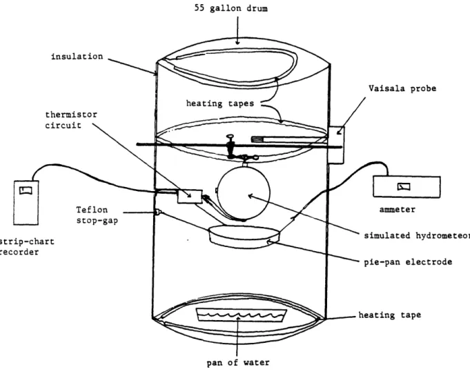
The principal experiments are conducted in a standard 55 gallon (.208

M3) stainless steel drum used as a miniature cloud chamber, shown in

Figure 1. The drum is covered on the outside with 1 inch fiberglass insulation secured with duct tape, and three Thermolyne heating tapes powered by variacs are used to achieve quasi-steady state temperatures in

the chamber. Environments warmer than room temperature can be

55 gallon drum insulation thermistor circuit N Teflon stop-gap strip-chart recorder Vaisala probe ammeter simulated hydrometeor pie-pan electrode heating tape pan of water

bottom of the chamber is filled with water pre-heated to the

environmental temperature to provide vapor for the frost growth. The temperature and relative humidity of the air in the can are continuously

monitored with a Vaisala Series HMP 11OA humidity probe mounted approximately 12 inches below the top of the drum.

Approximately level with the probe, a .375 inch diameter stainless steel rod is mounted through the drum and serves as the support for the cold simulated hydrometeor. A 9" diameter aluminum pie pan is centered several inches beneath the simulated hydrometeor to catch the splintering ice particles ejected and carried downward by gravity during frost growth. The pan is'electrically bonnected to 6 Keithl6y Model 410 picoammeter and thus is an electrode for the measurement of charge separation. Runs with

an ungrounded simulated hydrometeor connected directly to the ammeter yield numbers which are equal in magnitude but opposite in sign to the current measurements from the pie pan using a grounded specimen (An

example of this is shown in Figure 21 in the Interpretation section). Thus, we are confident that the plate indeed collects all of the charge carriers separated during a trial. The pie pan method of measurement is preferred because of the ease and quickness it affords in placing the simulated hydrometeor into the chamber and beginning a run. The pan-electrode is mechanically supported by strands of waxed dental floss tied to two .5" Teflon insulators glued to the drum wall. The Teflon is sufficient to

prevent leakage currents because there is no liquid water near the chamber wall at any time during an experimental run. Occassionally, the Teflon

accumulate on the insulator surface.

The ammeter is located outside the chamber and its input BNC is grounded to the metal drum, providing good shielding for the pan-electrode

The Keithley instrument has twenty settings between 1

OX1 0-4

The principal simulated hydrometeor used is a welded 6" diameter hollow stainless steel sphere (STS), manufactured by Weil Pump Co., Chicago, IL, filled with water to approximately 91% of its capacity (about

1800 ml) and then frozen. The sphere is supported by a .25" diameter

screw and thread assembly welded to the top. Other objects are used to explore the possible contaminating effect of metal type on the observed charge transfer. These include two six inch diameter hemispheric

aluminum cups (made from type 0 3003 Al by Carlstrom Pressed Metals, Inc., Worcester, MA, and subsequently referred to as AL1 and AL2) filled with 700 ml water and then frozen. Each is supported by three wires soldered through holes 120 degrees apart in the cup lip and centered and

soldered together above to an alligator clip. 6" diameter hemispheres of ice, formed by freezing distilled water to plastic supports within the 6" aluminum cups, give a true ice surface to test for charge separation. And last, a 6" diameter aluminum sphere made from two welded aluminum cups

of the above type is used for comparison with the 6" stainless steel

sphere. It is held up by a stainless steel hook attached to the top. Hence, during the experiments the metal simulated hydrometeors are grounded and so no charge can accumulate on their surfaces. The distilled water ice hemispheres, on the other hand, are floating electrically.

In the earliest experiments, a small (approximately 1.5" radius) copper planting cup supported by an alligator clip in the manner of the aluminum hemispheres was also used in a room temperature environment at high humidity and yielded results with the same general trends as the other metal simulated hydrometeors. Work with this specimen suggested that to get current values significantly above the noise of the ammeter for all test conditions, larger specimens and warmer chamber temperatures are desirable. This motivated the use of the larger 6" diameter stainless steel and aluminum simulated hydrometeors and the heating tapes for the

main body of trials.

The simulated hydrometeors are frozen in a thermostat controlled So-Low brand chest freezer capable of -50 degrees Celsius. They are generally frozen overnight to ensure that equilibrium with the freezer has been reached. Metal hydrometeor temperatures in the freezer are

monitored with Omega 44033 precision bead thermistors interchangeable to ±0.1 degrees C. The stainless steel sphere has two small hollowed stainless steel knobs welded to the outside, one at the equator and one on the bottom pole, where thermistors can be inserted and are removable. Similarly, the aluminum sphere has one hollowed aluminum knob welded to the equator. Thermistors sheathed and sealed in .875" sections of .125"

diameter copper piping, flattened and drilled at one end, can be screwed into holes at the lips of the aluminum cups for temperature determination. Unfortunately, a drawback of the distilled water ice hemispheres is the absence of a convenient means of accurately monitoring the surface temperature. In these experiments, we assumed that the ice temperature could be reasonably represented by the value of a thermistored, ice filled aluminum cup at the same height in the freezer.

A simple amplifier circuit (see Appendix A for diagram) in an aluminum

shielding box is mounted to the inside wall of the drum and connected to a strip chart recorder. Alligator clips serve as the connector between the circuit and the leads of a thermistor attached to the metal simulated hydrometeor used during an experimental run. The time constant for the Omega 44033 is about 10 seconds in still air and the dissipation constant, defined as the power in milliwatts to raise a thermistor 1 *C above the surrounding temperature, is on the order of 1 mw/*C. Hence, the most

important design consideration for the circuit is that it supply a minimal current to the thermistor. In this case it acts as a constant current source of approximately 15 microamps. The maximum resistance encountered in the experiments is 150 K, corresponding to about -50 *C. For this worst case, we have a power dissipation in the thermistor of .03 mW<< 1 mW, and therefore it can be neglected. Thus, a measure of the surface temperature during frost growth can be accurately and continuously recorded.

Finally, a small (.375" diameter) hole drilled in the side of the drum can be used, with the aid of a 40 Watt lamp set inside the chamber, to view the process of crystal splintering and ejection.

The typical procedure in an experimental run consists of first warming the drum to the desired temperature and then adding the heated water to build up the vapor supply to the desired level, which generally takes 30-45 minutes. It is important to allow the can to heat up for several hours before a run so that the drum walls and Teflon supports can come to equilibrium with the air temperature in the can. This prevents water from condensing on the insulators and causing leakage currents. When the appropriate relative humidity and temperature have been reached, a trace of the background current to the pie pan-electode is taken for several minutes to check for leakage currents and to determine the zero level on the Rustrak recorder. With this step successfully completed, the

simulated hydrometeor, which has been cooled to the desired temperature, is quickly removed from the freezer and placed into the chamber.

Generally, 15-20 seconds are consumed between opening the freezer door and getting a meaningful reading on the ammeter. Data is then taken until the frost grown on the simulated hydrometeor has melted.

There are obvious problems with the initial boundary conditions in this experiment. The procedure does not allow for rigorous reproducibility.

In placing the cold object in the drum, the cover must be partially removed, allowing drier room temperature air to mix with the chamber environment. The degree of mixing is dependent on the temperature difference between

the can and the outside and the length of time the lid is ajar. Also, the twenty odd seconds required for the transfer between the freezer and the chamber are lost data and represent an unknown variable which is not easily eliminated.

Probably more important than the variable initial condition, though, is the fact that the temperature of the cold object cannot be fixed during frost growth. In an experiment which is attempting to measure charge

transfer vs. temperature at which ice is splintering, this is of crucial

importance. However, the temperature difference between the simulated hydrometeor and the warm moist environment of the chamber is so great

(300C - 1 O0C) that, with this arrangement, it is impossible to maintain a

constant ice temperature. The only temperature value that we are

confident is a valid representation is the temperature of the surface of the object when it is in the freezer. Once in the drum, it becomes a

complicated heat transfer problem. The warmup behavior of a simulated hydrometeor is geometry dependent, and is also a function of position on the surface, and the temperature and humidity of the growth environment. Temperature can be monitored at several points on the metal surfaces during ice growth, as has been described previously, but at best it is an approximation of the value at other points on the metal and at the tips of the growing dendrites.

This leads to an obvious question as to why the experiment is set up in this manner. Clearly, such large temperature gradients are never

experienced by real graupel particles growing in a thunderstorm. We estimate that a graupel particle in a dry growth regime is probably never greater than 0.50C warmer than its environment while falling through a thundercloud (For details see Appendix E). The exaggerated growth

conditions also make analyses and conclusions very difficult. However, the most important consideration here is to be able to measure the

phenomenon with the instrumentation and equipment available, and it is within these constraints that the experiment evolved.

The main body of experiments is done with the chamber temperature (Tc) at 41 *C and the starting relative humidity (RHs), before the cover is opened to place the cold object inside, at 88% (vapor content - 50 gm/m3). This combination is chosen because it is a relatively easy-to-achieve

moist environment with a strong signal to noise ratio in the measured current. Runs are completed with the starting temperature of the cold object (Ts) ranging from 50*C all the way up to 0*C, in increments of 3

-60C, to test the dependence of the current measured on ice growth temperature. To establish repeatability and reliability, 3 or more trials at each starting temperature (Ts) are run for each of the simulated

hydrometeors.

To test for the dependence of electrical current on different vapor concentrations, a less extensive set of experiments with the aluminum

cups and the stainless steel sphere is conducted at Tc =28*C, RHs=93%

(vapor content ~ 26 gm/m3), or about one half of the above value. Also, a set of current measurements is run a Tc -520C, RHs -85%, vapor content 79 gm/m3_{, or about 1.5 times the vapor content of the Tc=41 OC runs, with} the stainless steel sphere only. These additonal runs focus on the

stainless steel simulated hydrometeor because, in the initial experiments, it was found that the current magnitudes from runs with this specimen appear more repeatable and consistent than for the other cold objects.

Data

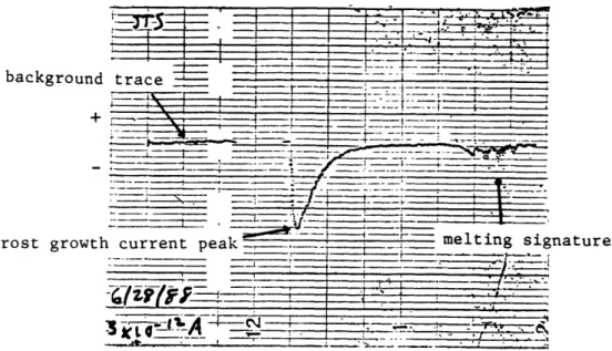
In the course of the experiments it was found that certain systematic features of the current vs. time plots are common to all runs with the metal simulated hydrometeors at all temperatures where a signal is detected (ie. where the signal to noise ratio is greater than 1 at a particular ammeter setting). An example of a typical Rustrak trace is shown in Figure 2. This particular run wa done at Tc =410C, RHs =88%,

Ts=-200C, with the 6" stainless steel sphere (STS). Four divisions

horizontally is equal to fifteen minutes, and one large division in the vertical is .6 X 10-12 amps (In all of the Rustrak traces shown in this

paper, five large divisions vertically are equal to the full scale of the instrument, and this number is always listed in the lower lefthand side of the trace). Negative charge from the sphere (and to the pie pan) is

represented by a downward deflection and the background zero line is at the left. The run begins at the abrupt drop of the recorder needle. Discrete 'samples' on the Rustrak are separated by 2 seconds. The maximum current value of -1.7 pA to the pan-electrode is reached approximately 30 seconds

into the experiment, as the simulated hydrometeor is charging positively. The current then tails off exponentially to zero at about 8 minutes and

remains there until the 'spike' at the end of the run which is associated with the melting of the frost growth.

backgrou

frost grow

id trace --- _________ ___

- - --- _ - ---- _ - ---- _ - - _

Figure 2 - Typical current trace for an experiment run, showing background current, peak associated with frost growth, and melting signature.

In all of the runs in which there is a measurable current (S/N >1 ), as in the example above, there is always a quick rise to the peak current at the start followed by an exponential decline to zero and then a second current

maximum associated with melting that signifies the end of the experiment. The two peaks are mutually inclusive, i.e. both are seen or there is no charge transfer detected at all (S/N =1 ).

There are also systematic features to all sets of runs with a particular simulated hydrometeor at one chamber temperature. Generally, the

maximum current increases with increasing temperature to some maximum value (Tsmax) and then decreases above this temperature. The time to maximum current, on the other hand, tends to decrease with increasing temperature up to Tsmax and then increases above this temperature. In other words, the highest peak currents are achieved in the shortest times.

Total run times increase with decreasing Ts at a given Tc and generally also increase with decreasing chamber temperature. These features are illustrated in Figure 3, which shows a partial set of runs done at Tc=280C,

RHs=93%. Again, in all of the traces, negative charge to the pan is downward, five large divisions is equal to 10X10 3 amps (1pA), and four divisions horizontally is 15 minutes. The runs start with a background trace at the left followed by the current profile. Note that the trial at

Ts=-20C is a straight line (S/N s1).

The finite time to maximum current does not seem to be a relic of the response time of the ammeter, but a real, systematic effect in the frost growth/charge separation process. The smoothness of the frost growth

+r _-_--. -- - -- r-w o -- ---£sbrr- -rA7 - - -n - _;- -_- - -- - - s.~ =57t = - - - ___.-_-_-- -w -- a z9 -- .-- - - - --- -3

-Figure 3 - Set of runs with STS at Tc=28*C, full scale = 1 pA.

peak suggests that the charge carriers from the simulated hydrometeor in this regime represent a near continuum of particles, whereas the melting signature appears to be a series of discrete events, recognizable within the response speed of the instrument. Also, in all of the runs using cold metal objects, the current to the pie pan is always negative (i.e. there is no temperature regime or time period during the growth and melting process in which there is a net transfer of positive charge from the simulated hydrometeors to the pie pan).

In the following we focus principally on the data from the stainless steel sphere, as it appears to be the most repeatable and consistent and thus amenable to analysis. Within the STS data we concentrate on the set of numbers from Tc=41 *C, RHs=88%, because this is where the greatest percentage of the trials are conducted.

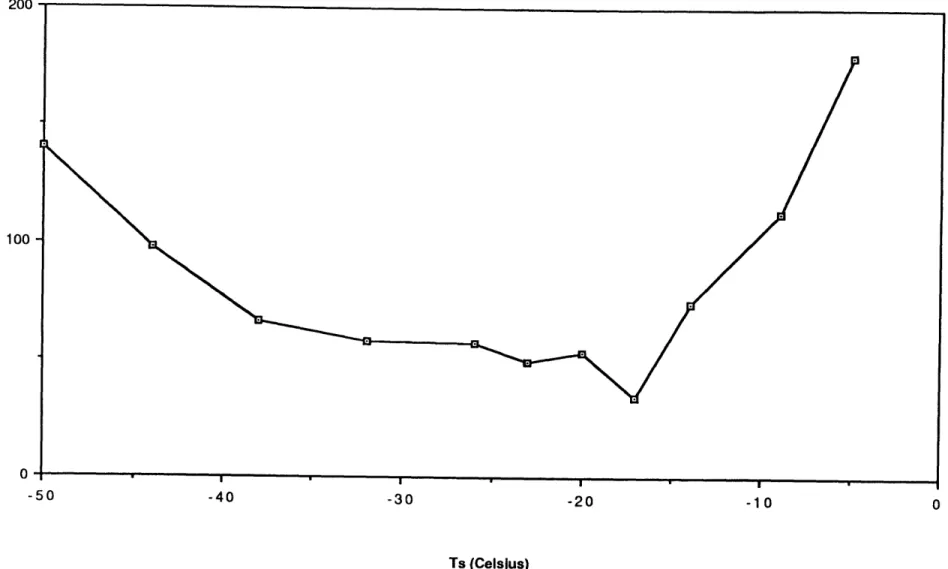
A plot of the maximum pie pan current (Imax) in the frost growth peak

vs. starting temperature (Ts) of the cold object for Tc =41 *C, RHs=88% is shown in Figure 4. Clearly, there is a strong and consistent dependence of

inax on Ts, with a pronounced peak around -170C. Imax appears to decrease monotonically for temperatures on the cold side of -1 80C down to the freezer limit of -50*C, where the values are about 20% of the maximum of -2.8 pA. Imax drops sharply for temperatures warmer than -1 70C but

there is evidence for a distinct 'shoulder' in the temperature dependence between -10OC and -50C. There is also an abrupt cut-off regime between -50C and -40C, where the charge transfer drops to zero. At -50C the frost

Figure 4 - Data from STS, Tc=41 C, RHs=88% 3- 2-0 -50 -40 -30 -20 -10 0 Ts (Celsius)

growth peak and the melting signature are distinguishable, while at -40C the Rustrak trace is a straight line (S/N 51, similar to Fig. 3). Visual

observations of these 'warm' T runs suggest that above -40C no real frost growth and ejection of ice splinters occurs, just condensation on the metal

surface.

Total run times between start and frost melt at 41 *C for STS range from 60-70 minutes at Ts=-500_{C down to about 7 minutes at Ts=-5 OC,}

where the growth peak and melting signature overlap.

For each of eleven Ts values,listed in Table 1, the times from the start of a run to Imax of that run (timax) from the current traces at that Ts are averaged to yield imax also listed in Table 1. Timax is greatest

(140 sec.) at Ts = -50*C and gradually shortens to a minimum value of

about 35 seconds at -170C. For Ts > -17*C, the average time to Imax then increases. These averages are also plotted in Figure 4A. Note, again, that the peak Imax value and the fastest timax occur at the same temperature.

For the experimental results plotted in Figure 4 there was no

monitoring of the surface temperature of the stainless steel sphere, as the connection of the thermistor amplifier circuit to the simulated

hydrometeor occassionally causes spurious current signals. Runs to determine temperature-time profiles of the warming stainless steel sphere were conducted in addition to the above, and the current

measurements from these trials were discarded. The temperature history of the bottom of the sphere was taken for the eleven Ts values between

Table 1 - Time (timax) and temperature (Tbimax) at the bottom of STS at Imax, Tc=41*C, RHs=88% Timax (sec) 140 98 66 58 57 49 53 34 74 113 180 Tbimax (0C) -44 -39 -34 -28 -22 -19 -16 -13 -10 -3 0 Ts (0_C) -50 'max (pA) .45 .60 .68 .86 -44 -38 -32 -26 -23 -20 -17 -14 -9 -5 1.00 1.57 1.94 2.72* .88 .56 .34

4 4)p

-40 -30 _{-20 -10 0}

Ts (Celsius)

Figure 4A - Average time to I

max vs. T for runs at T =41

0 C, RH =88%. s c s 200 100 -50 I'3

-500_{C and -5*C listed in Table 1. It is assumed that each profile}

represents the warming behavior of the sphere from the respective Ts, so that we can use this data to estimate an average temperature at the

bottom of the sphere at Imax for a particular Ts, Tbimax.

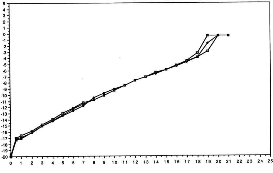
To demonstrate the repeatability of these temperature profiles, we present three warmup traces from Tc=41 C, Ts=-200_{C, RHs=88%, in} Figure 5. These plots are obtained as follows: The thermistor-amplifier circuit outputs a voltage which is proportional to the resisance of the thermistor (see Appendix A). Values from the voltage vs. time trace are then taken at 1 minute intervals and converted into numbers for electrical resistance . The conversion table from resistance to temperature for the Omega 44033 lists temperatures at increments of *C with a corresponding

resistance at each temperature. Thus, to convert our experimental resistances to temperature, we employ a cubic spline algorithm to interpolate between the table-supplied numbers.

Looking at the plots in Fig. 5, we see that for the duration of the runs, at any one time, the Tbottom values are always within .50C of each other.

Hence, we are confident that the single profiles obtained for each set of run conditions are a good representation of the temperature history of the non-thermistored, current measurement trials.

The value at t=imax on the temperature profile from the thermistor-amplifier at a particular Ts then yields Tbimax. We stress again that this is the temperature at one location on the sphere, at a knob soldered to the

lk1 0 F'

Figure 5 - Tbottom vs. time for 3 STS runs,Tc=41,Ts=28,RHs=88%

5 4 3 2-1 0-* -1--2 -3-I-4 -5 0 -6-E o -7--8 * -9--10 *1 -11 . -12 E E -13 -14 -15- 1617 --18 -19 -20 1 2 3 4 6 - 8 - 9 1 - 18-0 1 2 3 4 5 6 7 8 9 10 11 12 13 14 15 16 17 18 19 20 21 22 23 24 25 Time (minutes) AL V It p

bottom pole of the sphere, at the averaged time to maximum current in the frost growth peak for runs at one freezer starting temperature. This

measurement is as accurate a determination of the temperature at the base of the ice growth as is possible with the available equipment.

However, the bottom of the specimen is relatively insulated by the cold boundary layer, and hence, a question arises as to the validity of this area as a representation of the entire surface of the object during growth in the warm environment of the experiment chamber.

To examine this question, we mount STS with the two thermistors, one at the bottom and one on the equatorial knob, and compare the warmup profiles from the two sites. The run is done at Tc=41* C, RHs=88%, Ts=-170C. The plot of both temperatures vs. time is shown in Fig. 6. The zero of time is the time at which the electronics are turned on after the sphere has been placed in the chamber. The temperature plotted 20 seconds to the left of time zero is the temperature of STS in the freezer. Also plotted in the figure, with the dashed line, is a typical current trace from a run with those initial conditions.

In this data we see a substantial difference in temperature (4-70C) between the bottom knob and the side knob. Though the side knob is probably slightly warmer than the stainless steel surface at the equator, the sphere clearly does not warmup uniformly across its surface area, and thus Tbottom is not a good representation of the temperature at other points on STS during warmup in these run conditions. However, we will see in the next section that the ice crystal ejection activity appears to be

liEII

Cd

-4-)

Time (minutes)

Figure 6 - Temperature at bottom and temperature at side of STS vs. time for a run at Ts=-l7*C,

Tc=41*C, RHs=88%. Also shown is a typical current trace for a run at those conditions.

"'""""

RiinilH nlioli

.I I I I I . . .I I I . I

...

.

I

,

I

confined to a small region including the bottom of the sphere, so Tbottom probably is a valid indicator of the temperature at which charge separation is occurring

Returning to Table 1, we see that the Tbimax values are listed for all eleven specimen starting temperatures. The value in the table is rounded to the nearest degree C. Generally, Tbimax is increased by about 40C relative to the initial sphere temperature, Ts. The broad range of Tbimax is evidence that the current maximum is not simply the result of a growth independent phenomenon occurring at a unique 'resonance' temperature, as the frost growing on the simulated graupel particle warms through this

temperature. The charging phenomena appears to depend on the history of frost growth.

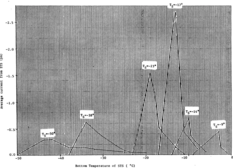
To more clearly illustrate this important point we have T vs. Tbottom plotted for a range of Ts values at Tc=41*C, RHs=88% in Figure 7. I is just the average of the currents from three independent measurements at a

particular time=t for the runs at that Ts. To determine the abscissae, we just take the Tbottom value at time=t from the temperature vs. time trace

at that Ts, Tc, & RHs (eg. Fig. 6). For each Ts trace shown in Fig. 7, the leftmost point is just the specimen starting temperature in the freezer and is assumed to have a current transfer of 0 pA.

The total charge transferred from the specimen to the pie pan

electrode during the frost growth peak can be determined by enlarging the Rustrak traces and using a simple graph paper square counting technique to

-2. 5 -2.0 0 $4 T -5 0-Bottom Temperature of STS ( C)

integrate the area under the current vs. time curve (assuming a continuum

process). Table 2 lists some values from the above data at Tc = 410C. The

table is not comprehensive because not all of the Rustrak data is amenable to this technique due to early calibration problems of the chart recorder. Though limited, it is useful. The spread in Q values is much smaller than that in Imax* In fact, the total charge transferred in runs at this chamber

environment is fairly constant below -170C, certainly with respect to the

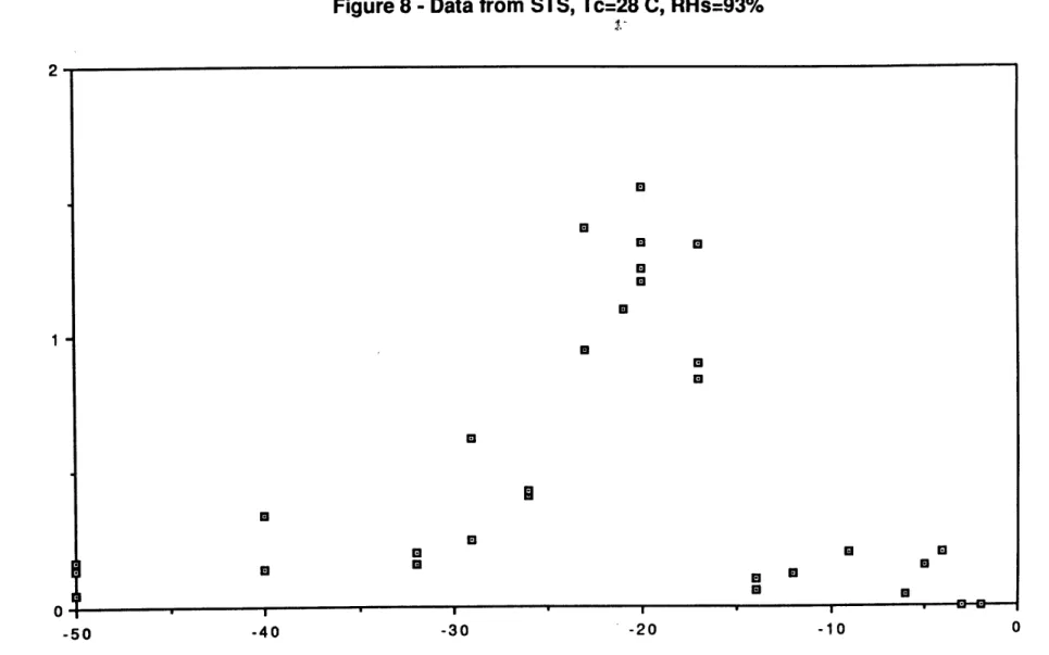
factor of five difference across Ts in maximum current values (See Fig. 4). Next we present the data from experiments done using STS with the chamber temperature at 280C, RHs=93%, which has a vapor content (26

gm/m3_{) about one-half of the value in the environment at Tc=41 C (50}

gm/m3_{). The Imax vs. Ts results for this less extensive set of runs are} plotted in Figure 8. Peak values of the maximum current occur around

Ts=-200C, about a factor of 7 greater than the numbers at Ts=-500C, which

are close to -.2 pA. The plot has the familiar trend seen in STS data at

Tc41* C, with a current cut-off temperature between -3*C and -40C. timax and Tbimax numbers are shown for 10 values of Ts in Table 3.

Iimax

Table 2 - Total charge transferred (Q) for STS, Tc=41 OC Q (pC) _{Qaverage (pA)} -310 -300 -200 -210 -220 -250 -290 -360 -380 -290 -150 -64 -40 -64 -310 -200 -210 -220 -250 -340 -290 -110 -52 Ts (*C) -50 -44 -38 -32 -26 -20 -17 -14

Figure 8 - Data from STS, Tc=28 C, RHs=93% 2-* H 0. 1- U U x 0 * M 0 - - - 1 0 - 50 - 40 - 30 -20 - 10 0 Ts (Celsius)

Table 3 - Time (imax) and temperature (Tbimax) at the bottom of STS at Imax, Tc=280C, RHs= 93% timax (sec) 213 265 211 112 84 76 87 197 170 330 Tbimax (*C) -45 -34 -29 -23 -21 -18 -13 -9 -6 -1 Ts (*C) -50 -40 -32 -26 -23 -20 -17 -14 -9 -4 Imax (pA) .13 .24 .19 .42 1.18 1.34* 1.03 .08 .20 .21

0 & k1 4k I' 'AO 0 0 0

-40 -30 -20 -10

Ts (Celsius)

Figure 8A - Average time to I _max vs. T for runs at T =28*C, RH _s =93%.

c s 400 300 200 100 -50

not the same as the value for Tc-41* C, being about 5*C colder at Tc=28*C than the Tbimax number of -1 3*C for the warmer chamber environment.

The third and smallest set of STS data is taken at Tc=520C, RHs=84%, a

chamber environment with approximately 1.5 times the vapor content of the Tc=41 C runs. The Imax vs. Ts plot for these trials, shown in Figure 9, exhibits much more erratic behavior than the numbers for STS at the lower drum temperatures. Still, the trend of increasing Imax with increasing Ts from -50*C is evident. Maximum currents of -12.0 pA and -10.5 pA are recorded at Ts=-21 *C and Ts=-23*C respectively, but it is difficult to discern confidently a peak response temperature in these data due to the substantial variance in the measurements. Note that the above two Imax values are approximately 4 times greater than the largest numbers at Tc=41 C, RHs=88%. Response times (timax) are significantly faster than for runs with Tc=41 C, ranging from about 1 minute for Ts=-50*C down to around 10-15 seconds for the maxima just below Ts=-2 *C. Such times are dangerously close to the response speed of the ammeter. Perhaps this is a contributing factor to the large variance in the Imax values at this high

can temperature. No sphere warmup temperatures were monitored during this set of trials.

To demonstrate that there are characteristics of the charge separation phenomena that appear to be indepedent of metal type used, we next consider data taken with the aluminum specimens as simulated

A # 4 P * 40 0 0

Figure 9 - Data from STS, Tc=52 C, RHs=84%

14 12 0 0 10-8 -U6 - M 4 -2 0 -50 -40 -30 -20 -10 0 Ts (Celsius)

hydrometeors. We have found that the aluminum electrodes yield results with a greater variance than runs with STS. This is consistent with

reports in the literature that aluminum is perhaps questionable for use as an electrode (Sill, 1963). Because of this we place less emphasis on analysis of the aluminum data.

First we present Imax vs. Ts plots for the two aluminum cups,

designated AL1 and AL2, at Tc=41*C, RHs=88%, in Figures 10 & 11. These results show systematic differences in the responses of the two cold

objects in several temperature regimes and thus we have kept this data separate and do not consider the two specimens interchangeable. The tinting of the two hemispheres is slightly different, but the supplier

claims that the manufacturing process and metal used has not changed to their knowledge. Perhaps the older cup, AL1, has become oxidized.

For both AL1 and AL2 there is similarity with STS in that Imax increases with increasing Ts from -50*C, though the variance in the values at any one freezer starting temperature is greater. Figure 10 suggests a maximum in Imax for AL1 near Ts = -32*C, with a systematic decrease at higher temperatures to a current cut-off value between -1 40C

and -90C (Again, Ts is the temperature at the equator of a hemisphere just

before it is pulled from the freezer for a run). The latter behavior is also followed by AL2. As was the case for the STS cutoff temperature, this seems to be the regime in which frost never forms on the cup surface, just condensation. The much lower cutoff temperature for the aluminum

Figure 10 - Data from AL1, Tc=41 C, RHs=88% 3-0 E 2-LUU 1-U 0 -50 -40 -30 -20 -10 0 Ts (Celsius)

* * *A

Figure 11 - Data from AL2, Tc=41 C, RHs=88%

3 U U a. 2-0 -50 -40 -30 -20 -10 0 Ts (Celsius)

cups is most certainly a result of a geometry-dependent difference in warmup behavior. In Figure 11, the position of the maximum is less well defined, lying somewhere between Ts = -32*C and Ts =-1 70C.

The Imax magnitudes for AL1 & AL2 at Tc=41* C are similar to STS.

Direct comparisons at specific Ts values are not meaningful, again, because the two geometries exhibit substantially different warmup

profiles. Total run times at Tc = 410_{C range from about 25 minutes at Ts}

=-50*C

about 90_{C warmer than Ts in this growth environment, yielding a value of}

-230C for the -320C Imax value for AL1. The value of Imax for AL2 lies in the -230_{C to -8}0_{C range; the large variance in the measurements may} obscure the more narrowly defined peak for STS (Fig. 4). The reasons for the greater variance in the measurements with the aluminum cups is still not understood.

The current vs. time profiles prior to melting for the aluminum

hemispheres are generally indistinguishable from STS profiles of a similar magnitude and Ts regime. In other words, the risetimes and Q values for AL1 and AL2 at Tc = 41 OC are about the same as for STS. An example to illustrate this is shown in Fig. 12. The -2.25 pA peak in fig 12a) is from an

STS trial at Ts=-200_{C, Tc=}4_{1* C, with a total charge separation (Q) of 360}

pC and a risetime of 55 seconds. The trace in Fig. 12b) is from one of the

+ t~---'---'--.- -

-~it P

(a)

(b)

Figure 12 - (a) current trace from STS trial at Ts=-20*C, Tc=41*C, RHs=88%, full scale = 3 pA, & (b) current trace from ALl trial

at Ts=-32*C, Tc=41*C, RHs=88%, full scale = 3 pA.

-2.4 pA and Q=370 pC, with a risetime of about 40 seconds.

As has been previously discussed, the current peak during frost growth and the melting spike are the standard signatures for runs done with the

metal simulated hydrometeors. However, trials at -440C and -500_C, especially with the aluminum hemispheres at Tc = 41*C are an exception to this rule. An example is shown in Figure 13. This run shows what appears to be two current peaks associated with frost growth. Also, for the spheres at these lowest temperatures studied, the initial current peak often decays in what appears to be a departure from the exponential behavior, and occassionally a second peak at Ts=-500_{C appears (For} example, see Appendix C). This effect shall be discussed further in the

Interpretation section.

As was the case with STS, the data with the aluminum hemispheres at Tc=2 80C is less extensive than at Tc=41'O. Imax vs. Ts at Tc=280_C,

RHs=93% for AL1 and AL2 are shown in Figures 14 & 15 respectively. The profile for AL1 at this temperature is similar to that with the same cup at Tc=41* C, but the maximum appears to be shifted to the right a few degrees Celsius, to around -290C. Tbimax for Ts=-290_{C is -23*C, which is the same} value of the bottom temperature at the average time of maximum current for the -32*C peak in the AL1 data at Tc=4_{1* C. The AL2 data at Tc=}280_{C do} not exhibit a narrow maximum, as was the case for runs at Tc-414 C, but points between Ts=-300_{C and Ts=-20}0_{C are clearly greater than the Imax}

_ e- ~

r/z r

Current trace from AL2 at Ts=-50*C, Tc=41*C, RHs=88%, example of double peak. Full scale is 1 pA.

Figure 14 - Data from ALl, Tc=28 C, RHs=93% 21 Eli Eil C, li. cc - ' -50 -40 -30 -20 -10 0 Ts (Celsius)

Figure 15 - Data from AL2, Tc=28 C, RHs=93%

21

0. 0

numbers on either side. Tbimax for Ts=-20*C for AL2 here is -15*C.

Maximum Imax currents in Figures 14 & 15 are about -1.4 pA, roughly half of the peak values seen in the aluminum hemisphere trials at T=41 O*C.

The Imax data for the 6" diameter aluminum sphere (ALS) at Tc=41 _OC, plotted vs. Ts in Figure 16, is even more erratic than the AL1 & AL2

results. Again, though, it is clear that the maximum current value broadly increases with decreasing Ts up to about -25*C and then decreases to nearly zero by -4*C. To be more specific is difficult in light of the large variance in these results. It is interesting to note that the highest currents recorded, nearly -2.0 pA at Ts =-26*C, are smaller than the largest Imax values of AL1 & AL2, which have smaller surface areas than the sphere. There is no Tbimax data for ALS, but the total run times agree closely with those of STS (also 6" diameter) at the same freezer starting temperatures, so the warmup profiles are probably similar. Also, as with the aluminum cups, current peaks associated with frost growth for ALS are indistinguishable from current peaks for STS of the same magnitude.

The last set of data to be discussed are the runs with the ice

hemispheres at Tc=4_{1* C. In earlier experiments it was determined that} results using Cambridge tap water ice are indistinguishable from distilled water ice trials. Distilled water is used only because it has a constant, known composition and is probably more representative of the composition of ice particles in the atmosphere. Though ice is a poorer thermal

Figure 16 -Data from ALS, Tc=41 C, RHs=88% 3 2-ti 1-El 0 MEl -50 -40 -30 -20 -10 0 Ts (Celsius)

results do show similarities with the data for the metallic simulated hydrometeors. An early current peak is a persistent feature. However, systematically at Ts=-240_{C, and several times at other freezer starting} temperatures, the current trace has a positive excursion in the first 10 seconds or so of the run and then reverses to the normal negative transfer to the plate. An example of this is shown in Figure 17. This sign change is generally difficult to discern because it occurs so quickly into a run that it is often unclear whether the signal is just the result of the settling down of the picoammeter after the cold object is placed in the chamber.

Moweverthe case in Figure 17, which is representative of s=-240Qfor the ice hemisphere runs, cannot be dismissed as an instrument response effect. The amplitude of the positive excursion fluctuates greatly from

run to run, sometimes going off the scale at the particular ammeter setting for the experiment. The limitations imposed by the initial boundary conditions make this phenomenon very difficult to quantify.

The Imax vs. Ts plot for the distilled water ice hemispheres at Tc=41 C

(See Fig. 18) does show an increase in Imax as Ts increases from -500_C that is not inconsistent with the metal data. The diamond data points are cases with a clearly discernible initial positive current deviation to the pan. The values shown are the maximum negative currents to the pan during the frost growth phase of a run. Obviously, the figure is not very useful as it stands. The variance in these measurements is even greater than the results for the aluminum cups in Figs. 10 & 11. We feel that the inconsistencies evident in this data are a direct result of the inability to

background

positive excursion

Figure 17 - Current trace for run with water ice cup at Ts=-24*C, Tc=41*C, RHs=88%, showing positive excursion in peak

associated with frost growth.

Figure 18 -Data from ice 'cups', Tc=41 C, RHs=88% 2-0 normal sign + excursion uU CLo 00 -50 -40 -30 -20 -10 Ts (Celsius)

monitor the ice temperature and to be certain of the surface state of the ice at the beginning of a run. For example, a slight temperature

disequilibrium with the freezer air, which is most surely present in a thermostat controlled freezer, can put the surface alternately in a state of evaporation or deposition, with consequent electrical effects. This is easy to identify and control on a metal surface, but not so with an ice surface.

This, combined with the uncertainty in the initial boundary condition makes further analysis of the distilled water ice data unrewarding.

Before proceeding to the next section, we must make some comments about the problem of controlling and determining the relative humidity during a run imposed by the experiment procedure. As was stated in the experiment section, the three temperature/moisture environments were chosen so that the ratio of the total vapor content in the chamber would increase roughly as .5 :1.0 :1.5 for the three temperature regimes: 280C,

410C, & 520C. This is assuming, of course, that RHs is a reasonable

representation of the relative humidity in the can during frost growth. However, again, when the drum lid is slid off, mixing occurs with the outside air, to an extent determined by how long the chamber is open, which is relatively constant from run to run (5-10 seconds), and also by the temperature contrast with the surrounding environment. It turns out that the relative humidity during the current peak associated with frost growth for different Ts runs at a particular Tc is fairly constant, usually within ±3%. Figure 19 shows a typical relative humidity vs. time trace for the beginning of a run at each of the three chamber temperatures. On the strip chart, one division horizontally is 30 seconds and 5 divs in the

-444---a.) TC- 28*C, RH - 93%, T -200C 1 div - 30 sec

b.) TC- 41*C, RH S 88%, T -17*C 1 div- 30 sec

ien

S[

c.) TC- 52*C, RHs 86%, Ts- -23*C 1 div - 30 sec

- position of for typical run

- FWHM for typical run

Figure 19 - Three chamber relative humidity vs. time traces with STS, one at each growth environment used in the experiment.

4

vertical is 10% relative humidity at that Ts. Runs begin at the right hand side with the sudden drop in RH. Fig. 19(a) is a trial at Tc=280C, Ts=-20*C,

RHs=93%, while 19(b) is done at Tc=41*C, Ts=-170C, RHs=88%, and 19(c) has initial conditions of Tc=520_{C, Ts=-23}0_{C, RHs=86%. Note that as Tc} increases, the initial drop in relative humidity increases as well, due to the increasing contrast between the air in the can and in the laboratory.

There are some interesting features that are common to all three of these traces. After the initial drop in RH caused by the uncovering of the chamber lid, the relative humidity is seen to rise for several minutes before falling steadily for the remainder of the run. This is undoubtedly due to the proximity of of the humidity sensor to the top of the can. The

upper layers of air are mixed most with the laboratory air, and when the chamber is once again closed, convective homogenization with the

relatively unmixed air at the bottom causes the apparent rise in relative humidity in the can. After this initial homogenization, the accumulation of ice on the simulated hydrometeor slowly depletes the vapor supply and hence the RH reading begins to fall. This is consistent with measurements of the mass growth on the sphere which will be presented in a later

section. For example, the can environment in trace (b)., for the .208 m3 can, yields a total water content of about 10 g. Our measurements of the

2-minute mass growth in this environment suggest growth accumulations after 5-10 minutes that should be an appreciable fraction of 10 grams, and this should be refelected in the RH trace. Note also in Figure 19 the short term, small amplitude variations in the signal, caused by the point source

(the water pan at the bottom of the chamber) and sink (the simulated hydrometeor) of water vapor in the presence of convective overturning.

Also shown in Fig. 19 for each RH trace is an arrow marking the time of a typical peak at that Ts and lines marking the full width at half

maximum (FWHM) for a typical current trace. Of course, the position of Imax and the FWHM will vary somewhat across Ts at one Tc, but if we assume the time periods around the FWHM's shown are representative of the times when, generally, most of the charge separation occurs, we see

that the average RH for 19a) is about 93%, while for 19b) it is

approximately 80%, and for 19c) the average is 68%. These three values yield total vapor contents of 26 gm/m3, 45 gm/m3_{, and 67 gm/m3}

respectively, or a revised ratio of .6 :1.0: 1.5 for the three principal can environments used in the experiments.

Further Observations

In analyzing the data presented above there are obvious and systematic features which we must attempt to account for. Clearly, there is a

substantial variation in average maximum current across Ts at any one particular growth chamber environment, and there is also a large variation

in Imax at a given Ts across the three principal chamber temperatures. Before addressing these trends, though, we will take a step back to examine information revealed in several supplemental qualitative

observations and quantitative measurements performed in an effort to answer more basic and general questions about the phenomenon. For example, Are we sure the charge carriers are, in fact, ejected ice

crystals?

The observation window drilled into the wall of the ice growth chamber proves to be a very useful tool for qualitative analysis of the charge separtion problem. ~A typical trial proceeds as follows: At the

start of a run, when the cold object is first placed in the drum, it is sheathed in an optically thick supercooled condensation cloud. The condensation boundary layer is relatively thin higher up on the simulated

hydrometeor, but near the bottom (perhaps 25 degrees from the bottom) it separates from the surface and forms a cylindrical flow shedding from the lower pole. The observed features of the flow are qualitatively consistent with numerical results for buoyancy induced single phase flows by

isothermal spheres (Gebhart,1987). The range of simulated hydrometeor sizeand chamber temperature in our experiments yields Grashof numbers (analogous to the Reynolds numbers of forced flows, See Eqn. 9, p.76) of

1 X 07 to 5X1 07 (See Table 4) for these experiments, with corresponding boundary layer thicknesses above the separation point on the order of 5mm (Gebhart, 1987, p.214).

Initially, there are no ice particles discernible in the flow, but as the frost becomes noticeable on the surface of the simulated hydrometeor, a

myriad of tiny ice fragments becomes visible reflecting in the chamber light. It appears that these miniscule particles emanate from the bottom of the sphere or cup, and that the middle and top facing areas are not involved. An example of the view from the observation hole of the ice fragment ejection from the bottom of the stainless steel sphere, with the condensation sheath and associated flow separation, is illustrated in

Figure 20.

As the frost growth progresses, chunks of dendritic structures,

perhaps 2-3 mm in diameter, are seen falling into the pan along with the tiny splinters. This is most evident in the runs at the lowest freezer

starting temperatures. Thick accumulation of frost is maintained on the inactive areas on the top and sides of the cold object, while from a critical angle (about 20* from the bottom) on the lower face down to the bottom pole, it appears the thick frost cannot be mechanically supported. This area is continually shedding large frosty snowflakes as the growth

becomes too heavy to be supported by the fragile dendritic trees.

Gradually, the ice fragmentation and the condensation cloud diminish in intensity, and as the simulated hydrometeor warms through O*C, the

accumulated ice starts to melt. The melting process is not instantaneous over the surface of the object, but starts from the top and advances slowly downward, taking as long as 5-10 minutes before melt water begins to drip from the bottom.

These visual observations suggest that the charge carriers in the

separation process are the miniscule ice particles described above. For a qualitative confirmation of this, two 3" diameter circular electrodes are

stainless steel sphere

flow separation

- ~ condensation sheath

r. _{ice crystals}

Figure 20 - Illustration of simulated hydrometeor in warm, moist environment of experiment chamber, with condensation sheath and ice crystals

ejecting from the bottom of the sphere.

mounted 10 cm apart in the chamber such that the ice crystals and

condensed cloud from a cold aluminum cup pass between them during frost growth. The electrodes are connected to a +1 kV supply. When the voltage

is applied, small ice fragments are deflected sideways and impact the positive electrode, indicating that they are negatively charged. It is difficult to discern if all fragments in the flow are deflected, but the condensation sheath appears unaffected by the applied field, as do the larger chunks of dendritic growth falling from the specimen.

Further visual evidence and measurements support the idea it is the small ice particles alone which are the charge carriers in these

experiments. In viewing a frosty specimen in the growth chamber, the'ice fragments can be seen falling into the pan under the weight of gravity. The

supercooled cloud billows over the pan edge, though, and thus a

considerable percentage of droplets do not ever come into contact with the pan-electrode. Hence, if the droplets were charged, the pan would not be registering the total current that was being separated from the

hydrometeor. Figure 21 shows two separate runs done with STS at

Ts=-1 70_{C, Tc=41 C, RHs=88%. Fig 21(a) is a standard trial with the pie pan} for electrical measurement, while 21(b) is done with the sphere connected directly to the ammeter, with the pan removed. The polarity of 21(b) has been reversed, and with this change, the traces are indistinguishable. Hence we can conclude that the pan is indeed collecting all of the charge carriers, which are the ice particles, and that the supercooled drops do not have a measurable charge.

+ .

T-(a)

(b)

Figure 21 - Two runs with STS at Ts=-17*C, Tc=41*C, RHs=88%, full scale = 3 pA. In (a) the ammeter is connected to the pie pan,

while in (b) the ammeter is connected directly to STS. Note the polarity is reversed in (b).

the pie pan current diminishes more rapidly in the initial growth peak than does the concentration of fragments ejected from the surface (i.e. When the current has already dropped off to near zero at a particular ammeter setting ten minutes or so into a run, there is still a substantial ice crystal 'snowstorm' beneath the simulated hydrometeor). Unfortunately, a quantitative measure of the relative intensity is not available.

This observation is evidence that the charge separation is dependent on the state of the surface from which the splinters are ejecting. More

specifically, it hints that somehow the initial deposition process of frost on a substrate is electrically active while later growth on a frost

substrate is inactive. A simple way to test this hypothesis is an

experimental run with a metal simulated hydrometeor that has a layer of frost already deposited on the surface at the beginning of the trial.

The test is done first with STS at Ts=-200C, Tc=280_{C, RHs=93%,} because this combination has a strong signal to noise ratio and yields consistent and reproducible results (See Fig. 8). The Imax values for this

set of conditions range from 1.2 to 1.5 pA (from the specimen). To prepare the sphere, the normal procedure for a standard current measurement run

is followed. STS is frozen to -20*C and placed in the chamber environment at Tc=280_{C, RHs=93%, and the ammeter needle is monitored. Approximately}

5 minutes into the trial, when the frost growth peak is essentially

complete and the pie pan current has returned to nearly zero (on the 3 X 10-12 A full scale setting), the sphere is quickly pulled from the drum and set back into the freezer.