Impact of global warming on ENSO phase change

(1)

HAL Id: hal-00296914

https://hal.archives-ouvertes.fr/hal-00296914

Submitted on 9 Jan 2006

HAL is a multi-disciplinary open access

archive for the deposit and dissemination of

sci-entific research documents, whether they are

pub-lished or not. The documents may come from

teaching and research institutions in France or

abroad, or from public or private research centers.

L’archive ouverte pluridisciplinaire HAL, est

destinée au dépôt et à la diffusion de documents

scientifiques de niveau recherche, publiés ou non,

émanant des établissements d’enseignement et de

recherche français ou étrangers, des laboratoires

publics ou privés.

Impact of global warming on ENSO phase change

W. Cabos Narvaez, F. Alvarez-Garcia, M. J. Ortizbeviá

To cite this version:

W. Cabos Narvaez, F. Alvarez-Garcia, M. J. Ortizbeviá. Impact of global warming on ENSO phase

change. Advances in Geosciences, European Geosciences Union, 2006, 6, pp.103-110. �hal-00296914�

(2)

SRef-ID: 1680-7359/adgeo/2006-6-103 European Geosciences Union

Advances in

Geosciences

Impact of global warming on ENSO phase change

W. Cabos Narvaez, F. Alvarez-Garcia, and M. J. OrtizBevi´a

Departamento de F´ısica, Universidad de Alcala 28871 – Alcala de Henares, Madrid, Spain

Received: 28 June 2005 – Revised: 31 October 2005 – Accepted: 14 November 2005 – Published: 9 January 2006

Abstract. We compare the physical mechanisms involved

in the generation and decay of ENSO events in a control (present day conditions) and Scenario (Is92a, IPCC 1996) simulations performed with the coupled ocean-atmosphere GCM ECHAM4-OPYC3. A clustering technique which ob-jectively discriminates common features in the evolution of the Tropical Pacific Heat Content anomalies leading to the peak of ENSO events allows us to group into a few classes the ENSO events occurring in 240 years of data in the con-trol and scenario runs. In both simulations, the composites of the groups show differences in the generation and devel-opment of ENSO. We present the changes in the statistics of the groups and explore the possible mechanisms involved.

1 Introduction

The El Ni˜no-Southern Oscillation (ENSO) dominates the in-terannual variability in the tropical Pacific atmosphere-ocean system and is the most important mode of variability in the present climate. Paleoclimate records show that ENSO has been a feature of the Earth’s climate for at least the past 130 ka (Tudhope et al., 2001), albeit with substantial changes in amplitude and frequency of the associated sea surface temperature anomalies through time (Rodbell et al., 1999; Woodroffe et al., 2003). An increase in ENSO amplitude can be detected in observed data for the last 100 years (Tudhope et al., 2001), with the events of 1982–1983 and 1997–1998 being the most intense in the observed record. Whether this increase in SST anomalies is related to enhanced greenhouse warming (Trenberth and Hoar, 1997) remains an open ques-tion. This is partly due to the difficulties in attributing the observed changes to CO2forcing rather than to interdecadal

variability, given the limitations in length and coverage of the observational record.

Correspondence to: W. CabosNarvaez

(william.cabos@uah.es)

In spite of some unrealistic features (Latif et al., 2001; Meehl et al., 2001), simulations with coupled General Cir-culation Models (CGCM) offer in many cases an adequate representation of present-day-like climatic variability, with the advantage of allowing an excellent data coverage in both space and time. They have thus become an essential tool in climate research and have been used to investigate, among other topics, the evolution of ENSO under different future scenarios. Model studies of greenhouse warming show a va-riety of results on this issue. For instance, an early simula-tion with a coarse resolusimula-tion model (Knutson, 1997), showed little change in ENSO-like activity in spite of a decrease in the mean zonal sea surface temperature gradient. In a cou-pled simulation with the HadCM2 model, Collins (2000) re-ports an increased frequency of ENSO events, and a shift in the seasonal signature. In another CGCM simulation, Tim-mermann et al. (2004) find that the increasing greenhouse gas concentrations induce a more El Ni˜no-like mean state, with more pronounced cold events than warm events. These changes appear to be related to an strengthening of the mod-elled thermocline (Timmermann et al., 1999).

In this study we investigate the possible effects of in-creased greenhouse warming on the ENSO-like variability found in the simulation already analyzed by (Timmermann et al., 2004), using a different type of analysis. By means of a clustering technique, we identify the main characteristics of simulated ENSO episodes when the model is forced accord-ing to the IS92a IPCC scenario (hereinafter SCR run) and compare the results with a second simulation with present day conditions (hereinafter CTR run). This technique has already been used to analyse ENSO characteristics in a sim-ulation of present day climate variability performed with an-other coupled GCM, the SINTEX model (AlvarezGarcia et al., 2005). Their study stressed the importance of decadal variability in ENSO generation and impacts. A recent obser-vational study of ENSO impacts, also based on cluster anal-ysis, draws similar conclusions (Potgieter et al., 2005).

(3)

104 W. Cabos Narvaez et al.: Impact of global warming on ENSO phase change:

2 Data

The ECHAM4/OPYC3 model (Bacher at al., 1998) is a cou-pled general circulation model. The atmospheric compo-nent, ECHAM4, is the fourth version of the European Cen-ter Hamburg Atmospheric Model. It is a spectral model that integrates the primitive equations (i. e., the fundamental equations that govern atmospheric motions) under the hy-drostatic approximation. In the simulation we analyze here, the atmospheric model variables are represented by spherical harmonics with the expansion truncated at wavenumber 42 (T42), equivalent to a 2.8◦_×_2.8◦ _{horizontal resolution. For}

a detailed description of the AGCM and its performance see R¨ockner et al. (1996).

The OPYC3 model is a layer oceanic model. It has the same zonal resolution as the atmospheric component and a variable resolution in latitude, enhanced to 0.5◦ near the equator. A more detailed description of the OPYC model can be found in Oberhuber (1993). The model is flux cor-rected and shows a good simulation of the seasonal cycle, the statistical characteristics of several climatic indices and the SOI-Ni˜no3 teleconnections. However, the model shows some deficiencies, such as the warmer than observed SST in the tropical Pacific off the South America coast and the over-estimation of the biannual component of ENSO.

The total length of both CTR and SCR simulations is 241 years, covering the 1860–2100 period. In the CTR simula-tion the concentrasimula-tions of greenhouse gases are fixed to their present-day values. In the SCR experiment the model was forced by increasing greenhouse gases concentrations from 1860 to 1990 and according to the IPPC Scenario IS92a since 1990.

3 Methodology

For this study we use a procedure capable of detecting classes of events (groups that share a distinct evolution), following the technique of AlvarezGarcia et al. (2005).

Our method compares the anomaly fields during the devel-opment of the events, and groups these on the basis of an ob-jectively computed measure of distance. The algorithm used seeks for common patterns in the development of different episodes. Thus, it does not attend only to their seasonality, amplitude, duration or any other simple condition. This way, our procedure is able to capture peculiarities of the ENSO episodes that are likely to be blurred by linear statistics tools such as Empirical Orthogonal Functions.

In a first step, with the help of the Ni˜no3 time series (SST average anomaly over [150◦W–90◦W, 5◦S–5◦N]), we iden-tify the ENSO events occurring in each simulation. We con-sider an ENSO episode occurs when the index rises over the one standard deviation threshold for at least 3 consecutive months. As an additional condition, we check that the event thus defined is coincidental with extremes in the first Prin-cipal Component of the tropical Pacific SST anomalies and in the atmospheric part of the phenomenon, as represented

by a model-adapted version of the SOI SLP anomaly index (difference between averaged SLP anomaly over [125◦_E–

135◦_{E, 20}◦_S–10◦_{S] and [155}◦_W–145◦_{W, 15}◦_S–5◦_S]).

For the classification, we consider for each event a 16 month segment, formed by 16 spatial maps, that ends with the peak anomaly in the Ni˜no3 index. The choice of this length owes to the two years period dominating the power spectrum of the simulated Ni˜no3 series. We monitor the event’s development in the evolution of the heat content (HC) anomalies in the Pacific basin within 15◦S and 15◦N. The HC is the energy stored in the upper oceanic layers and is defined in the point with coordinates (x,y) at time t by the equation

H C(x, y, t ) = Z 0

h0

ρcpT (x, y, z, t )dz (1)

where T is the temperature and the integration is carried out from the depth h0=300 m up to the ocean surface. To

com-pare different episodes, we compute a distance defined from the spatial correlation between their HC anomaly patterns in each of those 16 months. This distance serves as the basis for our classification, that is carried out by means of a two-step clustering technique. An initial classification is formed on the basis of a shared near neighbour criterion (Jarvis and Patrick, 1973). These initial classes are characterizad by a composite; they grow by gaining those elements whose dis-tance to the representative composite is below a fixed tresh-old. The procedure is repeated with an alternate definition of distance, in order to test the robustness of the classifica-tion. Before the classification, all (monthly) anomalies are standardized by their corresponding monthly standard devi-ation. We must take this step in order to adequately com-pare episodes with different timing. In the case of the SCR run, data have been detrended in order to remove long-term changes (that can be interpreted as variations of the back-ground state) from the anomalies.

Finally, each class is characterized by a composite event, formed by 16 spatial maps, representative of the class be-haviour.

An important issue in composite analysis refers to the se-lection of its significant features. We apply two significance tests: one on the group mean (Terray et al., 2003) and the other on the t-values (Brown and Hall, 1999). This second method makes use of robust estimators of the location (me-dian) and dispersion (interquartilic range) of the elements within a group which allows us to ensure we only retain those features that consistently appear throughout the class. In the following we comment only on features that pass both these tests at a 95% level.

4 Results

We have found 62 warm events in the CTR simulation and 66 warm events in the SCR simulations for the 240 years we analyze. We categorize the warm CTR episodes into three

(4)

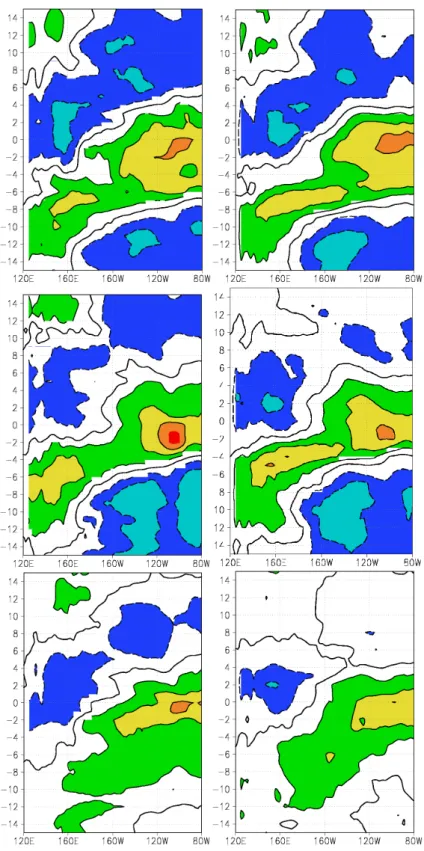
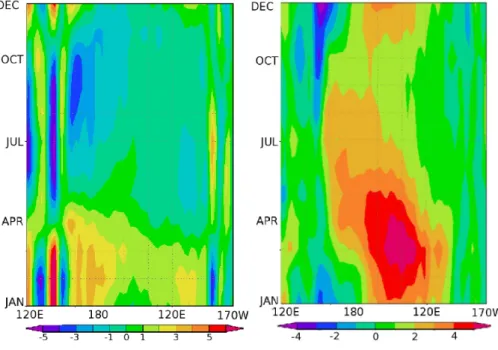
Fig. 1. Hovmueller diagrams of normalized Heat Content (HC) anomalies in the equatorial Pacific for the different classes of events found in the Control (left panels) and Scenario (right panels) runs. In the upper panels we represent the type 1 composites for both runs, the middle panels show the type 2 composites and the lower panels the type 3 composites. The HC anomalies are represented between 15 months before the events peak and 15 months after the peak. The contour interval is 0.5 standard deviations, negative values shaded in blueish colors. The zero label in time marks the month in which the Ni˜no3 Index of the SST composite of a given class peaks.

(5)

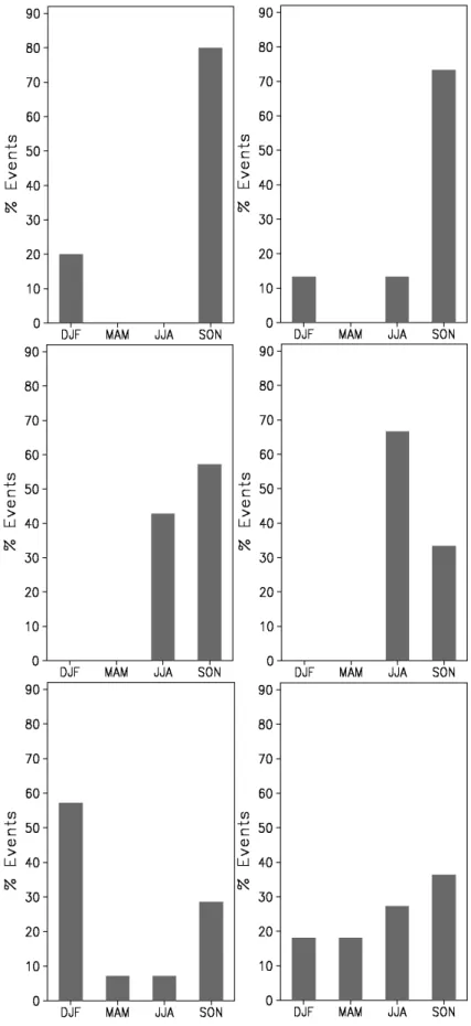
Fig. 2. The seasonal distribution of the peaking months for the events in the different classes identified in the Control (left panels) and Scenario (right panels) runs. As in Fig. 1, the upper panels represent the type 1 composites, the middle panels show the type 2 composites and the lower panels the type 3 composites.

(6)

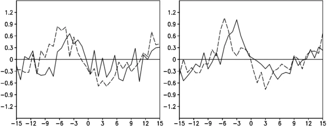
Fig. 3. The surface zonal wind anomalies in the Ni˜no5 region for the control (left panel) and the scenario (right panel) simulations. In both panels values for the class 1 in continous line and for class 2 in dashed.

classes: type CTR1, type CTR2, and type CTR3, respec-tively accounting for 49%, 17% and 34% of the classified events (10 warm episodes are not assigned to any group by our method). The SCR events are also distributed into three classes: types SCR1 (36% of the classified events), SCR2 (33%) and SCR3 (31%). 13 warm episodes are not assigned to any group by our method. Concerning the unclassified elements, most of them are too distant to any of the cluster centers (composites). There are also a few that lie relatively close to a certain class (cluster), in which they might have been included under a less restrictive choice of threshold dis-tances (see methodology above). We have preferred to keep this more restrictive thresholds for the sake of a greater con-sistency within the clusters.

We will use the equatorial HC (standarized) anomalies time-longitude diagrams of Fig. 1 for a short description of the CTR warm composites.

The CTR1 events are characterized by eastward propaga-tion of warm HC anomalies along the equator towards the eastern Pacific, formerly occupied by cold HC anomalies. This propagation begins about 10 months before the events reach their maximum. The events in this class peak mainly in boreal fall, with most of the events reaching their maximum in November (Fig. 2). Some events in this class peak in the DJF season.

The CTR2 events are in many aspects like those of class CTR1. The development of CTR2 episodes begins two months later than in the case of the CTR1 events, and the HC anomalies in the east equatorial Pacific have a shorter life span. For class CTR2, there are important positive anoma-lies in the surface zonal winds over the Ni˜no5 region (120 E– 140 E, 5 S–5 N) 8 months before the peak in Ni˜no3 Index. The case is quite different with class CTR1, as illustrated by (Fig. 3).

The events in the class CTR2 show a broader distribution in the seasonality of the peaks, that occur in boreal summer and fall (Fig. 2).

In contrast to the evolution of CTR1 and CTR2 events, the western equatorial Pacific HC anomalies play no part in

the generation of episodes of class CTR3. Previous cold HC anomalies in the eastern equatorial Pacific are also absent. Significant HC anomalies can be seen in the eastern equato-rial Pacific 8 months before the peak. The events of this class peak preferently in boreal autumn and winter, but a number of them do it in MAM and JJA (Fig. 2), so CTR3 peaks can actually occur in any season. We will not comment on these events, some of whose unrealistic traits remind of features in the simulation of the mean seasonal cycle in the eastern Pacific that need yet to be improved in coupled models.

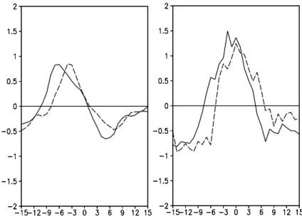
Turning to the SCR episodes, they are qualitatively sim-ilar to their CTR counterparts, as can be seen in Fig. 1. The distinction between classes SCR1 and SCR2, regarding the shorter development of class SCR2 and its tendency to peak earlier than SCR1 (Fig. 2), is somewhat clearer than in CTR. The differences between the type SCR1 and type SCR2 events can be also seen in the evolution of the equato-rial thermocline zonal-mean depth anomalies and the Ni˜no4 surface wind anomalies (Fig. 4): the development of SCR2 lags behind that of SCR1 by 2–3 months.

Though the classification essentially yields the same set of classes as in CTR, events distribute among the classes in a different way: the proportion of episodes falling in SCR2 grows (it practically doubles with respect to CTR) mostly at the expense of a decrease in the size of class SCR1. Further-more, SCR2 events concentrate in the last part of the SCR simulation (Fig. 5), which confirms the linkage between their relative abundance and the enhanced greenhouse gases forc-ing. Overall, the change detected by our procedure consists of a tendency of model ENSO episodes to shorten their de-velopment and peak one season earlier (in JJA rather than in SON) under SCR run conditions.

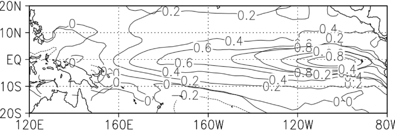
The greater occurrence of SCR2 events in the last part of the SCR simulation is associated with the modification of the background state. Fig. 6 illustrates the decrease in at-mospheric sensitivity in years 201–240 with respect to years 1-40, as measured by the difference between the regression maps of surface zonal wind anomalies on the Ni˜no3 index. This smaller atmospheric sensitivity might be due to the

(7)

Fig. 4. The Pacific equatorial thermocline zonal-mean depth anomalies(left panel) and the zonal wind velocity Nino4 Index (right panel) for the SCR1 (continous lines) and SCR2 (dashed lines) types.

Fig. 5. The first principal component of non detrended Sea Sur-face Temperature Anomalies for the scenario run and the peaking months for the SCR2 events (filled circles).

reduction of the surface wind convergence in years 201–240 (Fig. 7). Mean wind divergence has been pointed out in sev-eral works as a primary factor controlling the atmosphere-ocean coupling essential to ENSO variability (Tziperman et al., 1997) .

The reduced atmospheric sensitivity in the last part of the SCR run provides an explanation for the abundance of SCR2 episodes: the development of zonal wind anomalies is hin-dered, and hence the growth of the event, which leads to its premature peaking in JJA. Other changes in the mean state, such as the increase in SST sensitivity to Ni˜no4 (150 E–

150 W, 5 S–5 N) zonal wind anomalies (Fig. 8), must par-tially compensate this effect, since the amplitude of SST and HC anomalies does not diminish.

5 Conclusions

A clustering analysis is used to discriminate among the 62 warm ENSO events found in the equatorial Pacific in a global simulation of the climatic variability under present day ( CTR) and future ( SCR) conditions. The analysis detects three different behaviours in the generation and develop-ments of the warm ENSO events in the CTR simulation as well as in the SCR one.

The greatest difference occurs between events of class 1 (CTR1, SCR1) and 2 (CTR2, SCR2) and the events in class 3 (CTR3, SCR3). In the former two classes, there are HC anomalies in the western equatorial Pacific more than 9 months before the peak in the SST Ni˜no3 Index. These HC anomalies then propagate to the eastern Pacific. As opposed to this, in the latter class there are not any hints of accumu-lation of HC anomalies in the western equatorial Pacific, and subsequently no evident eastward propagation prior to the onset of the event.

But there are also significant differences in the way events of class 1 and of class 2 take place. The time span between the eastward propagation of the HC anomalies and the peak in the SST Ni˜no3 Index is greater (by 2 months) in events of class 1 compared with those in class 2. Another significant difference is the part that the far western equatorial Pacific plays in the generation of the events. In those of class 2, there are well developed surface zonal wind anomalies in the Ni˜no5 region 8 months before the peak. The surface zonal wind anomalies generate HC anomalies that propagate east-wards, a behaviour consistent with the one described by the

(8)

Fig. 6. Difference between the sensitivity of surface zonal wind anomalies to the El Ni˜no3 Sea Surface Temperature anomalies for the last 40 years and the sensitivity for the first 40 years of the scenario run.

Fig. 7. Seasonal cycle of the wind divergence at the equator for the first 40 years of the scenario run (left panel). Changes in wind divergence at the equator for the last 40 years of the scenario run with respect to the first 40 years (right panel).

“western Pacific oscillator” conceptual model. At this time (8 months before the peak) events of class 1 do not present such significant surface zonal wind anomalies in the Niño5 region. The accretion of HC anomalies in the western equa-torial Pacific seems to derive from different mechanisms in classes 1 and 2, which must be one of the factors influencing the differences in their subsequent evolution. Interestingly, zonal wind anomalies over the Niño5 region appear to be important again, now with reversed sign, in the mature stage of class 2 episodes, inmediately (around 3 months) after the peak in the SST Niño3 Index, but yet again not in class 1 (Fig. 3). Lastly, the seasonal signature in the peak of the Niño3 Index is more tightly linked to the end of the year in events of class 1, a feature observed in the real world.

The three classes are basically maintained under the sce-nario conditions, with three relevants modifications. One concerns the time span between the eastward propagation of

the HC anomalies and the end of the event, that is shortened by roughly two months for events in the classes 1 and 2. An-other is the distribution of the events among the classes, the number of events in class 2 comparatively increasing. And the last refers to the seasonal signature, that seems to be looser under the scenario conditions.

The relative abundance of episodes of class 2 in the last part of the SCR simulation might be connected with the rele-vance that wind anomalies over the far western Pacific (likely associated with SST anomalies in the area) appear to have for this type of events: the reduction of mean wind convergence decreases more effectively the sensitivity to SST anomalies in the central-eastern Pacific, where the SST mean state is cooler; this could emphasize the importance of processes in the far western Pacific and favour the generation of events of class 2.

(9)

Fig. 8. Difference between the sensitivity of Sea Surface Temperature anomalies to the El Ni˜no4 zonal surface wind anomalies for the last 40 years and the sensitivity for the first 40 years of the scenario run.

Acknowledgements. The authors wish to thank the Max Planck

Institute of Meteorology for the ECHAM4-OPYC3 data. This work was supported by the Spanish Ministry of Science and Technology through contract REN2002-02683/CLI.

Edited by: P. Fabian and J. L. Santos Reviewed by: two anonymous referees

References

AlvarezGarcia, F., CabosNarvaez, W., and OrtizBevi´a, M. J.: An as-sessment of differences in ENSO mechanisms in a coupled GCM simulation, J. Climate, accepted, 2005.

Bacher, A., Oberhuber, J. M., and Roeckner, E.: ENSO dynam-ics and seasonal cycle in the Tropical Pacific as simulated by the ECHAM4/OPYC3 coupled general circulation model, Clim. Dyn., 14, 431–450, 1998.

Brown, T. J. and Hall, B. L.: The Use of t Values in Climatological Composite Analyses, J. Clim., 12, 2941–2944, 1999.

Collins, M.: The El Ni˜no Southern Oscillation in the second Hadley Centre coupled model and its response to greenhouse warming, J. Clim., 13, 1299–1312, 2000.

Fedorov, A. V. and Philander, S. G.: A stability analysis of the trop-ical ocean-atmosphere interactions (bridging the measurements of, and the theory for El Ni˜no), J. Clim., 14, 3086–3101, 2001. Jarvis, R. A. and Patrick, E. A.: Clustering Using a Similarity

Mea-sure based in Near Neighbors, I.E.E. Transactions on Computers, C22, 353–399, 1973.

Knutson, T. R., Manabe, S., and Gu, D.: Simulated ENSO in a Global Coupled OceanAtmosphere Model: Multidecadal Am-plitude Modulation and CO2Sensitivity, J. Clim., 10, 131–161,

1997.

Latif, M., Sperber, K., Arblaster, J., et al.: ENSIP: the El Ni˜no sim-ulation intercomparison project, Clim. Dyn., 18, 255–276, 2001. Meehl, G. A., Gent, P. R., Arblaster, J. M., Otto-Bliesner, B. L., Brady, E. C.,and Craig, A.: Factors that affect the amplitude of El Ni˜no in global coupled models, Clim. Dyn., 17, 515–527, 2001. Neelin, J. D., Battisti, D. S., Hirst, A. C., Jin, F.-F., Wakata, Y., Yamagata, T., Zebiak, S. E., and Anderson, D.: ENSO theory, J. Geophys. Res., 103, 14 261–14 290, 1998.

Oberhuber, J. M.: Simulation of the Atlantic circulation with a cou-pled sea ice- mixed layer- isopycnal general circulation model. Part I: Model description, J. Phys. Oceanogr., 23, 808–829, 1993. Potgieter, A. B., Hammer, G. L., Meincke, H., and Stone, R. C.: Three putative Types of El Ni˜no Revealed by the Spatial Vari-ability in Impact on Australian Wheat Yield, J. Clim., 18, 1566– 1574, 2005.

R¨ockner, E., Arpe, K., Bengtsson, L., et al.: The atmospheric gen-eral circulation model ECHAM4: Model description and simula-tion of present-day climate, Max Planck Institut f¨ur Meteorologie Rep. 218, 94 pp., 1996.

Rodbell, D., Seltzer, G., Anderson, D. M., Abbott, M. B., Enfield, D. B., and Newman, J. H.: A 15 000 year record of ENSO-driven alluviation in Southwestern Ecuador, Science, 283, 516– 520, 1999.

Terray, P., Delecluse, P., Labattu, S., and Terray, L.: Sea surface temperature associations with the late Indian summer monsoon, Clim. Dyn., 21, 593–618, 2003.

Trenberth, K. E. and Hoar, T. J.: The 1990–1995 El Ni˜no-Southern Oscillation event: Longest on record, Geophys. Res. Lett., 23, 57–60, 1997.

Timmermann, A., Oberhuber, J., Bacher, A., Esch, M., Latif, M., and Roeckner, E.: Increased El Ni˜no frequency in a climate model forced by future greenhouse warming, Nature, 398, 694– 697, 1999.

Timmermann, A., Jin, F., and Collins, M.: Intensification of the annual cycle in the tropical Pacific due to greenhouse warming, Geophys. Res. Lett., 31, L12208, doi:10.1029/2004GL019442, 2004.

Tudhope, A. W., Chilcott, C. P., McCulloch, M. T., Cook, E. R., Chappell, J., Ellam, R. M., Lea, D. W., Lough, J. M., and Shim-mield, G.: Variability in ENSO through a glacialinterglacial cy-cle, Science, 291, 1511–1517, 2001.

Tziperman, E., Zebiak, S., and Cane, M.: Mechanisms of Seasonal ENSO Interaction, J. Atmos. Sci., 54, 61–71, 1997.

Woodroffe, C. D., Beech, M., and Gagan, M. K.: Mid-late Holocene El Nino variability in the equatorial Pacific from coral microatolls, Geophys. Res. Lett., 30(7), 1358, doi:10.1029/2002GL015868, 2003.