Common mechanisms for the representation of real, implied, and imagined visual motion

Common mechanisms for the representation of

real, implied, and imagined visual motion

by

Jonathan Winawer

City College

M.S., Neurobiology

of the City University of New York, 2005

B.A., Classics Columbia University, 1995

Submitted to the Department of Brain and Cognitive Sciences in Partial Fulfillment of the Requirements for the Degree of

Doctor of Philosophy in Cognitive Science

at the

Massachusetts Institute of Technology September 2007

© Massachusetts Institute of Technology 2007 All rights reserved

Signature of Author:

Department of Brain and Cognitive Sciences September 4, 2007

/

Certified by:

Lera Boroditsky Assistant Professor of Psychology Thesis Supervisor Accepted by: ASACHUS INSTITUTE. O EOHFNOOGY

Nov

2o0 2007

LIBRARIES

ARCHG

ES

-COMMON MECHANISMS FOR THE REPRESENTATION OF REAL,

IMPLIED, AND IMAGINED VISUAL MOTION

by

JONATHAN WINAWER

Submitted to the Department of Brain and Cognitive Sciences in Partial Fulfillment of the Requirements for the Degree of

Doctor of Philosophy in Cognitive Science

Abstract

Perceptual systems are specialized for transducing and interpreting information from the environment. But perceptual systems can also be used for processing information that arises from other sources, such as mental imagery and cued associations. Here we ask how a particular sensory property, visual motion, is represented when it is not directly perceived but only imagined or inferred from other cues.

In a series of experiments, a motion adaptation paradigm is used to assess directional properties of the responses to mental imagery of motion and viewing photographs that depict motion. The results show that both imagining motion and inferring motion from pictures can cause direction-specific adaptation of perceptual motion mechanisms, thus producing a motion aftereffect when a subsequent real motion stimulus is viewed. The transfer of adaptation from implied and imagined motion to real motion indicates that shared mechanisms are used for the perception, inference and imagination of visual motion.

Thesis Supervisor: Lera Boroditsky

Acknowledgments

It has been a great several years of graduate school, both at the Department of Brain and Cognitive Sciences at MIT, where I began graduate school and where I received my degree, and at the Psychology Department at Stanford, where I was a visiting scholar for the second half of my graduate career. I had the opportunity to learn from many people in these years, from Lera Boroditsky, my thesis advisor; from Alex Huk, who worked with me on all of the motion aftereffect studies; from Bart Anderson, my co-advisor for two years; from Nathan Witthoft, with whom I collaborated on much of my research as a graduate student; and from the many other faculty and graduate

students both at MIT and at Stanford. The collaborative spirit fostered in Lera's lab and at both universities provided an environment that both made good ideas possible and made doing science fun. Many research assistants also provided help over the years, and a particular thanks is owed to Jesse Carton for his help in the implied motion studies.

Table of Contents

Chapter 1: Introduction

Chapter 2: General Methods

Adaptation procedure with interleaved test stimuli Random dot stimuli and nulling

Fitting of curves with logistics Participants and equipment

Chapter 3: Motion Aftereffects from Imagined and Real Visual Motion

Experiment 3: Can a motion aftereffect from imagery be obtained with inward / outward motion?

Experiment 4: Does imagery-induced adaptation depend on reactivation from short-term memory?

Experiment 5: How do the motion aftereffects from imagined motion compare to those from real motion?

General Discussion

Chapter 4: Motion Aftereffects from Viewing Photographs that Depict

Motion

Experiment 1: Does viewing photographs that depict motion cause a motion aftereffect? Experiment 2: Does adaptation to implied motion, like adaptation to real motion, decline with a brief delay?

Experiment 3: Does adaptation to photographs with implied motion depend on the depiction of motion per se, or simply on the orientation of the scene?

Experiment 4: Does the implied motion aftereffect depend on eye movements?

Experiment 5: Can simultaneous viewing of real and implied motion cancel the effects of adaptation?

Experiment 6: Another means of measuring the motion aftereffect General Discussion

Chapter 5: Related Work and Conclusions

Does viewing a face with implied gaze lead to gaze adaptation?

Do macaque MT neurons show selectivity to the direction of implied motion? Conclusions

Chapter

1:

Introduction

Mental representations of objects and scenes and their properties may arise

through multiple processing routes. Bottom-up perceptual processing can bring a

stimulus to mind (say, looking at a face). But thoughts of the same stimulus can also be

triggered by an associated cue (hearing a voice or reading the person's name) or from

volitional imagery in the absence of any relevant perceptual input. To what degree are

common neural and psychological mechanisms used to represent such diverse thoughts?

In this thesis, I explore the nature of mental representations of one kind of

property, visual motion, arising from multiple routes: the perception of physical motion,

the inference of motion from action photographs, and mental imagery of motion. The

goal is to assess whether the latter two more abstract senses of motion - from inference

and imagery -- are built upon mechanisms used to perceive real motion.

To address this question, I ask whether direction-selective motion responses are

common to perceiving motion and to inferring or imagining motion: Does viewing a

photograph of a gazelle running to the left recruit neural circuits that respond selectively

to left physical motion? Does imagining an upward moving stimulus recruit neural

circuits that respond to upward real motion?

Mental Imagery

Overview and behavioral evidence. When asked to make a judgment about objects or scenes in long-term memory, like whether a pea is darker than a Christmas

tree, people often report that they form an image of the objects and inspect the image

more likely to fit through a door if is rotated on its side1_{. People may also try to vividly}

imagine events in order to rehearse for the future or to recall details about the past, such as whether windows were left open before having left the house.

Taken at face value, these examples might seem to be acts of recapitulating perceptual processes, but many theorists have questioned the degree to which such an idea is sensible, necessary, or even possible (Fodor, 1981; O'regan & Noe, 2001;

Pylyshyn, 2002). If the goal of perception is to arrive at an interpretation of sensory input (which is meaningless when uninterpreted), and the goal of imagery is to re-access the meaningful interpretation, why reproduce the whole process during imagery? This and related questions have spawned a tremendous amount of research into trying to determine experimentally precisely what properties and mechanisms constitute mental imagery, with a significant, ongoing debate between researchers with opposing views (e.g, Kosslyn, 1994; Pylyshyn, 2003).

An important study in 1910 demonstrated that mental imagery of a particular stimulus (e.g., a banana) and a dim and blurred visual presentation of the same stimulus were frequently confused by participants (Perky, 1910). Further explorations of the "Perky effect" have shown that even low-level visual tasks such as vernier acuity can be impaired during imagery of similar stimuli (Craverlemley & Reeves, 1987). Such results have been taken as evidence that "the materials of imagination are closely akin to those

of perception" (Perky, 1910).

But what "materials" of perception? Information in the perceptual processing streams may be represented at various degrees of abstraction, from cells tuned to the

1 Or, for me, since moving to the San Francisco Bay area, whether my car will roll into the street or onto

spatial location and orientation of luminance edges (Hubel & Wiesel, 1959) to cells that

respond preferentially to a particular movie star, whether presented as a photograph or as

a written name (Quiroga et al., 2005), akin to the abstract "grandmother cells"

hypothesized by Letvin (Gross, 2002). Thus another important question about imagery is

not just whether it is similar to perception, but the extent to which mental images contain

metric properties, as opposed to being fully abstracted representations.

Building on an observation of Ernst Mach in 1866, Roger Shepard and colleagues

conducted an elegant set of studies to demonstrate quantitatively that mental images

contain metric properties (Shepard & Cooper, 1982; Shepard & Metzler, 1971). In

particular, Shepard and colleagues demonstrated that when trying to determine whether

two objects are the same or different, subjects mentally align them, such that the time to

make the determination is remarkably well described as a linear function of the angle of

misalignment. Further studies have shown that the time it takes to shift one's focus from

one part of a mental image (e.g., the tail of a cat) to another part (its ear) is proportional

to the distance of the parts (Kosslyn, 1973). Such results are part of a tradition of clever

experiments which have sought to reveal the properties of mental images though indirect

psychological tests. These experiments have demonstrated that mental images have a

number of "image-like" properties typically associated with bottom-up perception,

including size (Kosslyn, 1975), resolution (Finke & Kosslyn, 1980), visual angle (Farah

et al., 1992; Kosslyn, 1978), and even a contrast-sensitivity function that varies with dark-adapted and light-adapted states (D'Angiulli, 2002). The wide range of studies

demonstrating shared, metric properties between imagery and perception, however, has

analogy and not shared processing. This has led imagery researchers to consider additional evidence from cognitive neuroscience.

Neural evidence. One principal finding from the cognitive neuroscience literature is that visual mental imagery can activate visual cortical areas in a modality and a feature-specific manner. For example, imagining visual stimuli activates visual cortex and can suppress auditory cortex (Amedi et al., 2005). Imagining visual motion activates

the cortical area MT+ (Goebel et al., 1998; Grossman & Blake, 2001) which processes

real visual motion. Imagining faces or places activates brain regions that are more

responsive to perception of the corresponding stimulus (O'Craven & Kanwisher, 2000).

Moreover, visual imagery can activate early, retinotopically organized cortex (Kosslyn et

al., 1999; Kosslyn et al., 1995; Slotnick et al., 2005).

Other sources of evidence have added to the functional imaging literature to make

the case that not only are perceptual brain areas activated during imagery, but the

activation plays a functional role during imagery. For example, disruption to early

occipital areas by transcranial magnetic stimulation interferes with imagery-based

judgments of visual attributes (Kosslyn et al., 1999). Furthermore perceptual deficits

from focal brain damage are often accompanied by corresponding deficits in imagery, though there are also cases in which the deficits are dissociated (for review, see Farah,

1989).

However, the neuroimaging and neuropsychological evidence leaves many

questions open regarding the perceptual mechanisms involved in mental imagery. For

example, consider the topic of this thesis, visual motion: one cannot infer whether mental

the same subsets of neurons, with similar tunings, are activated for imagined motion and

physical visual motion. fMRI measures net activity, and does not currently have the

resolution to routinely resolve individual columns. Moreover, although area MT+ has

been shown to carry direction-selective signals in response to visual motion (Huk &

Heeger, 2002; Huk et al., 2001), it can also be activated by other factors like attention and

arousal (Beauchamp et al., 1997; Corbetta et al., 1991; O'Craven et al., 1997; Saenz et

al., 2002) that may not be directionally-selective (Huk et al., 2001). Thus, a net increase in MT+ activation during imagery (Goebel et al., 1998) need not imply the existence of a

direction-selective signal, nor do multiple instances of MT+ activation confirm that the

same direction-selective neurons have been repeatedly activated (Grill-Spector &

Malach, 2001; Huk & Heeger, 2002). One of the two main aims of this thesis is to

address these questions, and we return to them shortly.

Perceptual inferences

In addition to mental imagery, which is typically a purposeful, voluntary act,

perceptual features can also be brought to mind in more automatic ways, even when not

directly perceived. Perhaps the most famous example is that of Pavlov's dog, in which a

sound was made to condition an anticipatory response in the expectation of food. Of

course the conclusion that the dog actually thought of food or any of its sensory

properties upon hearing the bell is antithetical to the basic approach of behaviorist

science, in which the goal was, at least in part, to characterize the input-output relations

without the need to make hypotheses about mental states. Nonetheless, such a possibility

seems reasonable and the idea that associative learning can have effects on perception has been pursued more directly by cognitive and perceptual scientists. For example, Qi and

colleagues (2006) trained subjects to associate an arbitrary stimulus with a direction of rotational motion, and found that following training presentation of the cue biased the perception of an ambiguous motion stimulus. In what might be thought of a natural experiment in associative learning, Cox and colleagues (2004) showed that photographs of human bodies with a smudged oval above it (instead of a face) activated a region of visual cortex that responds selectively to faces, the fusiform face area (Figure 1). The body and the configural cues in the image may be a well-learned indicator to the likely presence of a face, just as a Pavlov's bell may have indicated the likely delivery of food.

Figure 1. An example of a stimulus reprinted from (Cox et al., 2004). The contextual information in the image provides information that a face is present. Stimuli such as these were shown to activate face-selective regions of visual cortex.

Representational momentum. An example in the domain of visual motion is the

extrapolation of motion paths from images. Inferring motion trajectories is important for acting efficiently in dynamic environments. Even visual stimuli which do not contain motion but only imply it, such as frozen motion photographs, lead to the rapid and

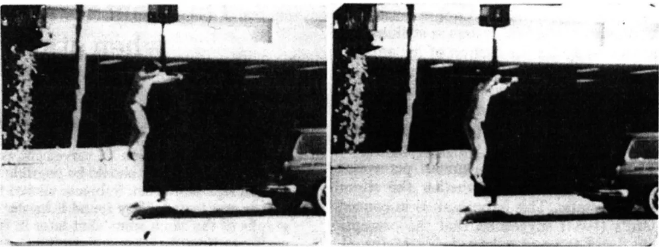
automatic extrapolation of motion paths (Freyd, 1983). In Figure 1 one can see a person

jumping. The sense of motion must be inferred from prior knowledge since there is of

course no physical motion in the photograph. Such stimuli would appear to have little in

common with the drifting dots and gratings commonly used to study neural mechanisms

of motion processing, other than the fact that the observer knows that both types of

stimuli depict motion in some sense. How is the sense of motion from photographs

represented in the brain?

Figure 2. An example of a stimulus reprinted from (Freyd, 1983). When subjects briefly viewed2an image like the one on the left, and then were tested with a similar image slightly later (like the one on the right) or slightly earlier from the same video clip, subjects were slower to say that the later picture was different from the original. This was taken as evidence that the later image was confused with the first image, presumably because subjects automatically extrapolated ahead upon seeing the first image. In later reports this and related phenomena became known as "representational momentum" (Freyd & Finke, 1984).

Form and motion. The primate brain contains a number of visual areas involved in the analysis of moving objects and patterns (Maunsell & Newsome, 1987; Tootell et al., 1995). Such areas contain neurons that respond powerfully in a direction-selective manner to moving images (Dubner & Zeki, 1971; Heeger et al., 1999; Huk et al., 2001). The direction of motion, however, may be inferred not just from analysis of visual motion but also from low-level visual form cues such as motion streaks (Burr & Ross, 2002; Geisler, 1999) or higher-level cues such as the posture of a person in motion (as in Figure

·--··~~ ~"ii71 (~-~'~~--· t~ · " · :·ii ·--r ·":- :Y ·· I· · -( I 2· 1

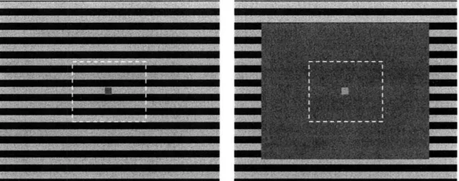
-3). In the case of low-level form cues it is thought that early visual processing such as the orientation-tuned cells in primary visual cortex can extract the relevant information and contribute to downstream motion processing. How high level semantic cues from objects and scenes might contribute to motion processing is less well understood. Is the sense of motion derived from such static cues instantiated by the same neural and psychological mechanisms as those subserving the perception of physical motion? In particular, we sought to test whether viewing implied motion images recruits the same direction-selective neural circuitry used for analyzing real visual motion. For example, does viewing the still photograph in Figure 3 elicit responses from the same leftward-selective neurons that would respond to real leftward motion?

Figure 3. An example of an implied motion photograph used in the experiments in Chapter 4.

Neuroimaging studies have shown that brain areas used to analyze physical motion are also activated by viewing implied motion stimuli (Kourtzi & Kanwisher, 2000; Lorteije et al., 2006; Peuskens et al., 2005; Senior et al., 2000). In these studies, viewing photographs or silhouettes of animals, people, objects or natural scenes

containing implied motion elicited greater activation in visual motion areas, most notably the MT/MST complex, than viewing similar images that did not imply motion (e.g., a cup

falling off a table compared to a cup resting on a table, or a running athlete compared to an athlete at rest). These studies demonstrate that implied motion, like imagery of motion, can activate brain areas also known to be engaged by real image motion. However, as in the case of mental imagery, one cannot infer from such studies whether viewing stimuli with implied motion elicits directional motion signals in the brain2. In order to infer whether the same neural circuits are employed by imagery and perception in the domain of visual motion, we made use of a motion aftereffect paradigm.

Motion aftereffect

The motion aftereffect or the waterfall illusion is a striking and well-studied perceptual phenomenon. It occurs when prolonged viewing of motion in one direction affects the perception of motion in subsequently seen stimuli. In particular, a static object or directionally ambiguous motion appears to move in the direction opposite to the previously seen motion. Motion aftereffects have been observed at least as far back as Aristotle, although not until Lucretius in the first century B.C. was the direction of the aftereffect unambiguously described as being opposite to the prior motion (see (Wade & Verstraten, 1998)). Both descriptions were of aftereffects from water flowing in a stream. The phenomenon was rediscovered a number of times in the _{19 th} century, most famously by Robert Addams whose observation of the Fall of Foyers in Scotland led to the name "Waterfall Illusion"; shifting his gaze from prolonged viewing of the falling water to the nearby rocks led to an illusory upward motion "equal in velocity to the falling water". A

2 _{Very recently, while in the late stages of editing this thesis, a study using EEG has shown}

direction-selective responses to implied motion (Lorteije et al.). This study provides independent, convergent evidence (though using very different methods) that implied motion and real motion processing share some direction-selective mechanisms. It is discussed further in Chapter 4.

comprehensive review of 19th century studies, as well as 34 original studies, was later

published in 1911 by Wohlgemuth for his doctoral dissertation.

Many explanations for the illusion have been offered, but an important component of many of the explanations, including that hypothesized by Wohlgumeth (1911) and measured by Barlow and Hill (1963), is the activity-related change in responsiveness of motion sensitive neurons. In this view the aftereffect results from the adaptation-induced decrease in activity of directionally selective neurons that respond to the adapted

direction of motion. This direction-selective adaptation in turn causes an imbalance in the population activity of neurons that represent different directions of motion. Because of this post-adaptation imbalance, the neural population code will indicate a net direction of motion opposite to the adapted direction when probed with stationary or directionally-ambiguous stimuli. Thus, the presence of a motion aftereffect can be used as a test for the involvement of direction-selective neural mechanisms (Kohn & Movshon, 2003;

Petersen et al., 1985; Van Wezel & Britten, 2002).3

Moreover, one can vary properties between the adapting stimulus and the test stimulus in order to make inferences about the representation of motion. For example, if a motion stimulus is viewed through only the left eye and a static test stimulus is

subsequently viewed only through the right eye, one will experience a motion aftereffect. This interocular transfer demonstrates through a simple behavioral observation that at 3 It is worth noting that an understanding of the neural and psychophysical basis of the motion aftereffect remains far from complete. For example it has recently been demonstrated that shifts in the directional tuning of motion sensitive neurons may be at least as critical for explaining the aftereffect as reductions in the magnitude of responses (Kohn & Movshon, 2004). Perhaps because of the difficulty in achieving a single, unified explanation of the phenomenon, Edward Adelson described the motion aftereffect to me as "A quagmire, a miasma, and a morass" (personal communication). It is not the purpose of this thesis to arrive at a mechanistic explanation of the motion aftereffect, nor do the experiments rest on the

assumptions of any particular model of the effect. Instead, the transfer of the aftereffect from one condition to another is used to infer the existence of shared representations between the conditions, without regard to exactly how adaptation occurs, or how motion is processed.

least some motion processing must take place centrally (not in each eye separately). More

generally, one can make inferences about the properties of neural circuits by measuring

whether adaptation transfers from one stimulus to another. Because of this, aftereffects

have been an important tool for studying perception (e.g., Gibson, 1933; Gibson, 1937;

Held, 1980)) and have famously been described as the psychologist's microelectrode

(Frisby, 1980). Hypotheses

We predicted that if visual imagery of motion is subserved by the same

direction-selective neural mechanisms that are involved in the perception of physical motion, then

actively imagining motion should adapt these neurons and produce a motion aftereffect.

Similarly, if viewing photographs of implied motion also uses the same

direction-selective neurons that are involved in perception, then viewing a series of such photos

depicting motion in the same direction would likewise adapt direction-selective neurons

and produce a motion aftereffect. We tested these hypotheses in a series of experiments

where we measured whether imagining continuous motion in one direction, either with

the eyes open or closed, altered the perceived direction of subsequently presented real

motion (Chapter 3); and in a series of experiments in which we measured whether

viewing implied motion in one direction altered the perceived direction of subsequently

presented real motion (Chapter 4). We also compared these results to baseline

Chapter 2: General Methods

Adaptation with interleaved test stimuli

The procedure for all the experiments had the same basic structure: prolonged

adaptation with interleaved test stimuli. Adaptation, depending on the experiment and

condition, could consist of mental imagery, viewing partially occluded motion, viewing

photographs with implied motion, or viewing real visual motion.' In order to maximize

the effect of adaptation, the direction of motion adaptation was always constant within a

block of trials. The first trial in each block contained a long period of adaptation (60 s)

and subsequent trials contained "top-up" adaptation periods of 6 s each. The logic is that

the initial adaptation trial in each block builds up an adapted state and counters any

residual adaptation from previous blocks of trials, and the subsequent trials maintain the

adapted state. The direction of adaptation changed between blocks. Between periods of

adaptation, brief test stimuli consisting of moving dots were presented to the subject, and

a forced choice judgment on the direction of dot motion was made (e.g., left or right). By

maintaining adaptation for a long period in one direction, a range of different test stimuli

can be presented to the subject and repeatedly tested. This procedure - a long initial

period of adaptation, followed by shorter top-up periods with interleaved test stimuli

-has been widely used to assess adaptation to a variety of stimulus types, including spatial

frequency (Blakemore & Sutton, 1969), motion (Hiris & Blake, 1992), tilt (Wolfe, 1984),

and, more recently, the gender or race of faces (Webster et al., 2004).

1 Note that for consistency and simplicity, the word "adaptation" is used in reference to each of these experimental conditions; in fact, whether direction-selective motion mechanisms are indeed adapted by a particular task, such as imagery, is the hypothesis being tested, and not an assumption.

Figure 1. A two-frame schematic depiction of a random dot test stimulus. In this example 4 of

10 dots (indicated in red) move coherently downward from frame 1 to 2. The other 6 dots

disappear and are randomly repositioned. In frame 2, 4 new dots are selected at random to move downward. This "limited lifetime procedure", in which new dots are selected randomly in each frame, prevents subjects from tracking individual dots to make a judgment on the direction of motion. Instead, subjects rely on a global sense of motion. The size, number, and luminance of dots and the frame-to-frame step-size are purely schematic. Detailed descriptions of the stimulus properties are in the methods section of each experiment.

Random dot test stimuli

The effect of adaptation on motion perception was assessed in all experiments (except experiment 6 in Chapter 42) with a standard moving-dot direction-discrimination task (Newsome et al., 1989; Newsome & Pare, 1988). Random dot displays such as those used in this task (Figure 1) have been important for studying visual motion systems because they do not contain recognizable features that can be used to infer a change in location over time, and are thus thought to rely on primary motion-processing

mechanisms, as distinct from processing of shapes or spatial positions (Anstis, 1970; Braddick, 1974; Nakayama & Tyler, 1981). In our versions of these displays, most of the dots served as noise, disappearing and then reappearing in a new location from frame to

2 _{For this experiment, a directionally ambiguous flickering stripe pattern was used as the test stimulus.}

frame. A proportion of the dots, however, moved coherently in a particular direction.

This proportion, or "motion coherence", varied from trial to trial, as did the direction of

coherent motion. The direction of coherent motion was always either the same as or

opposite to the direction of adaptation. Subjects were thus forced to choose one of two

directions in their judgments. The task is easy when the coherence is high and hard when

the coherence: is low.

Predicted shift due to motion adaptation

Probability of

upward

responses

motion coherence

Figure 2. Hypothetical motion sensitivity functions following adaptation. The null points (dashed vertical lines) are shifted to reflect motion aftereffects: following upward motion adaptation, a downward aftereffect is nulled by upward coherence in the test stimulus, and vice versa following downward motion adaptation. The separation between the null points (double-headed arrow) is a convenient measure of the aftereffect.

Nulling the motion aftereffect

This type of stimulus has been previously employed as a means to assess and quantify motion aftereffects from adaptation to real motion (Blake & Hiris, 1993; Hiris &

Blake, 1992). By varying the level of coherence from trial to trial as well as the direction of coherence (same as or opposite to adaptation), a motion sensitivity function can be extracted (Figure 2). From this function, one can easily find the point of perceived null motion, that is the amount of motion coherence for which the subject is equally likely to judge the dots as moving in the two opposite directions. The logic is that motion

adaptation (say to upward motion) produces an aftereffect in the opposite direction (downward). The aftereffect can be nulled by a fraction of dots moving coherently in the direction opposite the aftereffect. Thus adaptation can then be assessed as the difference in the null points between paired conditions, such as adapting to upward motion and to downward motion.

Using dynamic dot test probes as a method for assessing motion aftereffects has several advantages. First, by testing a range of coherence values and measuring the shift in the motion sensitivity function, the aftereffect is measured in units of the stimulus and not behavior (a "stimulus-referred" method): The size of a motion aftereffect can be expressed as the amount of dot coherence that must be added to a test stimulus following one kind of adaptation to make it perceptually equivalent to the same stimulus following

another kind of adaptation. This contrasts with the kind of measure one gets if only the neutral point is tested, e.g., by making a judgment on a static stimulus or a fully

ambiguous stimulus after adaptation. The units in the latter kind of measure are the increased (or decreased) likelihood of making a particular response, a measure in units of human behavior and not stimulus dimensions.

Additionally, dot probes are useful because they give subjects an objective task: there is in fact more motion in one direction than another on any given trial. All subjects

who participated in these experiments were na'ive to the purpose of the experiment. The

wide range of coherence values tested allowed us to validate that subjects were in fact

doing the task, in that their responses were predicted (in part) by the actual motion of the

test stimulus. In the occasional case in which this was not true, subjects were excluded

from analysis (see below).

Finally, dynamic dots are an advantageous stimulus because, at least according to

some reports (Blake & Hiris, 1993; Hiris & Blake, 1992), they can perceptually null a

motion aftereffect. If one adapts to motion (saw downward) and experiences a motion

aftereffect (upward), then a dot stimulus with partially coherent motion in the opposite

direction (downward) can counter the aftereffect such that it appears to have no coherent

motion. In other words, illusory motion can be perceptually neutralized with actual

motion coherence in the opposite direction. In contrast, a test object that has illusory

motion due to a motion aftereffect cannot be made to look static by adding motion in the

opposite direction. One possible explanation for this is that when motion is added to a test

object, the observer can still tell that the position changes, even if the motion is nulled,

creating a cue conflict. Because there are no stable edges or object parts in the dot

stimulus, there may be no cue conflict between the motion system and a system tracking object location.

Fitting of curves with logistics

The responses to random dot test stimuli were modeled as a logistic regression fitted with a maximum likelihood algorithm (Cox, 1970; Palmer et al.):

P(x) = 1 / (1 + exp(Y)),

In this equation, x is the motion signal in units of coherence, with positive values arbitrarily assigned to a particular direction, such as upward, and negative values

assigned to the opposite direction. P(x) is the probability that the subject judges the dots as moving in the positive direction (e.g., upward). A is the direction of adaptation (+1 or -1) and a, fl, and y are free parameters.

The free parameters correspond to an overall bias to respond in a particular direction (a), the steepness of the psychometric functions with respect to motion

coherence (f3), and the effect of adaptation (y). Dividing 2y by f yields a measure of the separation between the paired curves in units of coherence (e.g., the length of the double-headed arrow in Figure 2). The same bias (a) and slope (f3) were assumed for all

conditions for each subject to reduce the number of free parameters in the model. In some experiments subjects adapted to multiple types of stimuli, not just multiple directions. For example, in Chapter 3, Experiment 1 had occluded motion and motion imagery, and Experiments 2 and 3 had imagery with eyes open and with eyes

closed. For these experiments, an additional pair of terms, Y2 and A2, were added inside

the exponential corresponding to the additional adaptation condition:

P(x) = 1 / (1 + exp(Y)),

where Y = -(a + f3*x + y*A + y2*A2)

In the first experiment, for example, A corresponded to imagery adaptation (-1 or +1 for downward or upward imagery, respectively) and A2 corresponded to occluded motion

adaptation (-1 or +1 for downward or upward occluded motion, respectively). During imagery A2was 0 and during occluded motion blocks A was 0.

Subjects and equipment

Equipment and displays. All experiments were conducted in a quiet, dark room. Subjects were: seated approximately 40 cm away from the display, an Apple iMac with a

built-in CRT :monitor, with a resolution of 1024 x 768 pixels (26 x 19.5 cm) and a refresh

rate of 75 Hz. All experiments were programmed using Vision Shell stimulus

presentation software, a package developed at the Harvard Vision Lab that uses C

libraries and runs on the Macintosh OS 9 operating system.

Participants. All subjects were recruited from either the MIT or the Stanford

community. Subjects at MIT were paid for participation ($5 for 30 minutes or $10 for 60

minutes). Subjects at Stanford were either paid the same amount or received course

credit. All subjects gave informed, written consent, and all experiments conformed to the

university guidelines for human subjects testing, either at MIT (Committee on the Use of

Humans as Experimental Subjects) or at Stanford (Human Research Protection Program).

Exclusion criteria. A small number of subjects in each experiment did not show a significant effect of motion coherence. For these subjects, irrespective of the direction or

type of adaptation, the likelihood of judging a test stimulus as moving in a particular

direction (say, up) did not significantly increase with increased dot coherence in that

direction. Specifically, the parameter estimated for motion coherence in the logistic fit (B)

was less than two standard errors of the same parameter estimate. Additionally, a small

number of subjects performed poorly in a baseline motion discrimination task prior to

adaptation. For these subjects, curve fits showed that asymptotic performance (99% accuracy on the direction judgments of the dots) required more than 100% coherence in

Chapter 3: Motion Aftereffects from

Imagined

and Real

Visual Motion

The experiments in this chapter comprise a manuscript in preparation by Jonathan Winawer, Alex Huk, and Lera Boroditsky.

Abstract

Mental imagery, like perception, has distinct modalities. For example, one can

imagine visual properties of an object such as color or acoustic properties such as pitch.

Does the experience of these properties during imagery reflect underlying computations

similar to, and shared with, those used during sensory processing? Or is the connection

more abstract, with little shared between imagery and perception other than the fact that

they sometimes both concern the same thing? The studies in this chapter take advantage

of a well-studied feature of perceptual processing, directional responses to visual motion.

A series of experiments addresses whether imagining a moving pattern, like viewing real

motion, can elicit a motion aftereffect assessed with real motion test stimuli.

In the first study, subjects either imagined a pattern move up or down with their

eyes open, or passively viewed a large occluding rectangle around the periphery of which

a moving pattern could be seen. Both imagery and viewing occluded motion led to a

motion aftereffect, such that dynamic dot test probes were more likely to be seen moving in the direction opposite of adaptation. A second study demonstrated that aftereffects

could be obtained from motion imagery whether the eyes were open or closed during

imagery. This finding was replicated and extended in a third study in which subjects imagined horizontal motion either inward or outward, ruling out the possibility that aftereffects from imagery were coupled to eye movements. To investigate whether these effects were restricted to imagery of items in short-term perceptual memory, a fourth

experiment was conducted in which subjects had only limited exposure to the real motion patterns to be imagined. A motion aftereffect was observed in this experiment as well,

suggesting that imagery of motion can engage perceptual motion mechanisms without relying on short-term stored representations. Finally, motion aftereffects from real visual motion were assessed using similar methods to quantify the magnitude relative to

imagery.

The transfer of adaptation from imagined motion to perception of real motion demonstrates that at least some of the same direction-selective neural mechanisms are involved in both imagination and perception of the same kind of stimuli.

Experiment 1: Can mental imagery of a moving stimulus produce a motion

aftereffect?

In the first experiment, our primary question was whether imagining a moving grating, either upward or downward, could elicit a motion aftereffect. In the imagery condition of the experiment, subjects actively imagined a moving grating while fixating a central fixation square. Motion aftereffects were assessed with random dot test probes presented between periods of imagery.

In a second condition, we asked whether a motion aftereffect could be elicited by having subjects fixate a central occluder around which a moving grating could be seen.

This condition was not directly relevant to the hypothesis that mental imagery recruits direction selective motion mechanisms because subjects were not instructed to imagine. But because the dynamic dot test stimuli appeared in a small region in the center of the large occluded region where there was no motion, a motion aftereffect in this condition would indicate a non-retinotopic motion aftereffect. This condition served as an

intermediate between perception of motion and imagery of motion, and also as a way to

re-familiarize subjects with the appearance of the grating to be imagined. It is also served

as a partial replication of prior findings of non-retinotopic motion aftereffects (Bex et al., 1999; Snowden & Milne, 1997; Weisstein et al., 1977).

A pilot study was conducted on 6 subjects, and then a follow-up study with 32 new subjects. The follow-up was identical to the pilot in every respect except for slight

differences in the baseline motion sensitivity test and the selection of coherence values of

the test stimuli.

Methods

Subjects and equipment. 38 subjects, na've to the purpose of the experiment, were recruited from the MIT community. Subjects provided written consent and were paid for

participation.

Figure 1. Adapting stimuli for Experiment 1. Each stimulus filled the screen. The stimulus on the left, which could move either upward or downward, was shown to subjects prior to the adaptation blocks The "timing guide", or central fixation square pulsated with the average luminance of the stimulus passing behind it. On occluded motion trials, a large gray rectangle filled 75% of the screen (right). On imagery trials, the occluder filled 100% of the screen, such that there was no visible motion. The dashed white lines indicate the size of the test area with random dots. The figures are drawn to scale.

Adapting stimuli. In the beginning of the experiment, subjects were shown

examples of the moving stimulus that they were later to imagine (Figure 1). The stimulus was a square wave horizontal luminance grating with a spatial frequency of about .5 cycles per degree. The grating moved either upward or downward at a speed of 20 per second. Subjects were instructed to attend carefully to the appearance and speed of the grating (while fixating a central square, approximately 1o) so that they could later

imagine the grating as accurately and vividly as possible. In order to facilitate continuous motion imagery, the intensity of the fixation square was modulated, matching the average luminance of the grating passing behind it. The pulsating square, which contained no net directional motion, had the same temporal frequency as the grating. After this

familiarization stage, the pulsating square, shown alone on an otherwise blank screen, was used as a visual timing guide for motion imagery with eyes open.

In the occluded motion condition, a gray rectangle, 75% of the width and 75% of the length of the display occluded the grating, such that the moving grating was visible in the periphery (upper, lower, left, and right 12.5% of the screen).

Dynamic dot test stimuli. Test stimuli consisted of 100 dots contained within a

rectangular window, centered on the screen, whose length and width were 33% of the entire display (approximately 12 by 9 degrees of visual angle). On each frame a subset of the dots, equal to the percentage of dots moving coherently for that trial, were selected to move up or down. All other dots disappeared and randomly reappeared at any other

location within the test window. A new set of dots was re-selected for coherent movement on each frame. This "limited lifetime" procedure was used so that the

of 25 frames displayed for 40 ms each (1 s total). Dot displacement for coherent motion

was approximately 0.07 degrees per frame.

Baseline motion sensitivity. The experiment began with a baseline motion

calibration task. For the 6 pilot subjects the dot coherence in the baseline task was ±6%,

±12%, or ±24% over 48 trials, where positive numbers are arbitrarily assigned to upward motion and negative numbers to downward motion. These same 6 coherence values (3 up

and 3 down) were used for test stimuli during the adaptation blocks. These values were

chosen because pilot testing on the author showed that accuracy asymptoted at or below

about 24% coherence.

Because performance on the baseline task was highly variable among the pilot

subjects, a wider range of coherence values was used for the remaining subjects. For

these subjects the test values for the experimental conditions were chosen according to

performance on the baseline task, such that test stimuli were approximately perceptually

matched across subjects. The baseline task consisted of 180 trials, during which dot

coherence ranged from 5% to 65%, either upward or downward. A logistic function was

fitted to the responses, with downward coherent motion coded as negative and upward

coherence coded as positive.' Based on the fitted logistic function, the amount of

coherence corresponding to 99% accuracy in each of the two directions was determined

for each subject (Figure 2). The average of the these two unsigned values was considered

the maximal dot coherence for each subject, and defined as one unit of "normalized

coherence". The test stimuli presented during the adaptation phase of the experiment

'For simplicity of programming, the logistic function for the baseline task was fit using a least squares method, and not the more typical maximum likelihood procedure. Specifically, the logistic was transformed into a line, in which the x variable was the motion coherence and the y variable was the log odds of the responses (0 for "down" responses and 1 for "up" responses). These fits yield slightly different parameters than the estimation by maximum likelihood, but they are quite close.

contained ±0.25, ±0.5, or ±1 units of normalized coherence. Note that while the amount of coherence producing 99% upward responses and the amount producing 99%

downward responses was not necessarily symmetric (as in the example in Figure 2), the actual test values used in the experiment were always symmetric, in order to avoid the possibility of the test stimuli themselves inducing a motion aftereffect.

100% 75% -50% 25% -0% ... Q ... 0" -25 downward 0 25 50 upward

percentage of dots moving coherently

Figure 2. Baseline motion discrimination task for a single representative subject. The task consisted of up/down judgments on dot stimuli (x-axis, downward dots arbitrarily assigned to negative coherence values). The coherence values producing 99% responses based on the logistic fit (smooth curve) in each direction are indicated by dashed vertical lines. For this subject the values are 49% upward coherence and 43% downward coherence, averaged to 46%.

For this subject, 46% upward coherence was defined as one unit of normalized coherence, and was the maximally coherent test stimulus seen during the subsequent experiment. The 6 test stimuli viewed by this subject, ±1, +0.5, and +0.25 "normalized" coherence, correspond to ±46%, +23%, and +12% actual coherence.

Procedure. The instructions were programmed as part of the experiment to ensure that all participants received the identical instructions, and to minimize the possibility of

experimenter bias. Subjects first viewed 6 examples of high coherence dot displays to

familiarize them with the kind of judgments to be made (3 up and 3 down). This was

followed by the baseline motion discrimination task. Subjects then viewed the

full-screen moving grating twice in each direction (up and down) in order to familiarize them

imagery

adaptation (60 s)

imagery re-adaptation (6 s each)

Figure 3. Experimental procedure. Subjects imagined a moving grating pattern while fixating a small pulsing square. The direction of adaptation and whether the block contained imagery or occluded motion was constant within a block and randomized across 8 blocks of 24 trials. The first trial in each block consisted of 60 s of imagery or occluded motion adaptation, and

subsequent trials had 6-s top-up adaptation. Moving dot test stimuli were presented after each period of adaptation, and subjects made a two alternative forced choice decision as to the direction of the dot motion (up/down).

The adaptation phase consisted of 4 imagery and 4 occluded motion blocks, with two upward and two downward blocks of trials for each type of adaptation. There were 24 trials per block with each of the 6 coherent values being presented 4 times. Each block began with a 60-s adaptation trial followed by 6-s top-up adaptation trials (Figure 3).

Imagery trials began with the appearance of a static grating and a small arrow indicating the direction of subsequent motion imagery. The grating and arrow

immediately began to fade into gray, taking 1 second to disappear. The subject then imagined motion on a screen that was blank except for a fixation square. On alternate blocks, subjects either imagined motion or fixated a central occluder around which the moving grating could be seen.

At the end of the experiment, subjects were given a brief questionnaire adapted from the Vividness of Visual Imagery Questionnaire (VVIQ) (Marks, 1973). The questionnaire is a self-reported assessment of the vividness of mental imagery. Subjects are given a series of verbal descriptions of scenes, faces, and objects, and asked to vividly imagine each of them with their eyes open and then again with their eyes closed. After imagining each scene, subjects choose a 1-7 score corresponding to their self-assessed vividness of imagery. We also asked subjects two additional questions: Have you ever

heard of the 'Motion Aftereffect' or 'Waterfall Illusion' before, and After viewing upward motion, would you expect a static image to appear to move up or down.

Results and Discussion

Pilot subjects. In the pilot study we found that both imagining motion and

viewing occluded motion produced significant motion aftereffects. Imagination of

upward motion led to a greater likelihood of seeing the dynamic dot test stimulus moving down compared to imagination of downward motion. The same pattern was observed for viewing occluded motion. These patterns can be clearly seen in the population motion sensitivity curves, which show the mean results for the 6 pilot subjects (Figure 4). Had there been no effect of imagery or viewing occluded motion, each pair of curves would overlap. If subjects had answered based on an association (e.g., with a bias to respond upwards following upwards imagery) then the difference between the curves would have

been in the opposite direction than what was actually observed. These results are consistent with the hypothesis that imagery of visual motion involves some of the same directional-selective motion processing circuits also used for perception of motion.

lUU-/O 90% O 80% CL L 70% 60% 50% o 40% 30% S20% - 10% 0%

100% * downward occluded motion

e 90%

80% o upward occluded motion

o _a~ 80% _I a 70% o 60% 0 50% k4-o 40% 30% . 20% 0. 10% I0% -50 -25 0 25 50 -50 -25 0 25 50

motion coherence of test stimulus motion coherence of test stimulus

Figure 4. Population motion response functions for 6 pilot subjects following upward or

downward imagery (left), or viewing upward or downward occluded motion (right). Subjects were more likely to perceive upward motion in the test stimulus following downward imagery adaptation or viewing downward occluded motion. Data points represent the mean likelihood of responding upward ± 1 standard error of the mean. The x-axis is the motion coherence. Positive

numbers are arbitrarily assigned to upward motion. Curve fits are logistic regressions, with the slope constrained to be the same in each fit.

However, it is also evident from the data shown in Figure 4 that the subjects' responses were not greatly affected by the coherence in the test stimuli, that is the slopes are quite shallow. This means that the range of coherence in the test stimuli was not well matched to the range of the subjects' motion sensitivity, making it difficult to accurately estimate each subject's sensitivity function. In fact, an analysis of the individual subjects

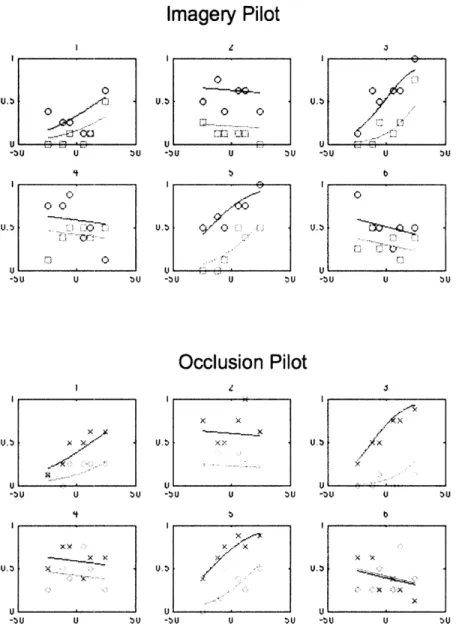
shows a split: collapsing across the imagery and occluded motion conditions, 3 subjects show significant sensitivity to motion coherence (subjects 1, 3, and 5) and 3 do not

(Figure 5). A significant effect of motion sensitivity was defined as a z-score of at least 2 for the motion coherence parameter on the logistic fit. (See General Methods.)

Imagery Pilot

Occlusion Pilot

Figure 5. Individual motion response functions for 6 pilot subjects following imagery (top), or viewing occluded motion (bottom). Red indicates downward imagery or occluded motion, and green upwards.. Each subject showed an effect in the predicted direction, being more likely to see the dots as moving upward following downward adaptation compared to upward adaptation, as predicted by a motion aftereffect. However, there is high variability between subjects in their motion sensitivity, with some subjects showing flat slopes (poor sensitivity to motion coherence) and some showing steep slopes (good sensitivity).

Normalized coherence. These results suggest that the range of coherence values in

the test stimuli was far too restricted for some subjects, but reasonably good for others. For the remaining 32 subjects (as well as all subjects in subsequent experiments), the coherence values used during adaptation were chosen to be equivalent with respect to subjects' motion sensitivity as determined in the baseline (see General Methods). Once

SU - U U tU

0o

the sensitivity was determined from the baseline, the maximal coherence used during adaptation was considered one unit of "normalized coherence". Comparing the size of a normalized unit of coherence in the main experiment and the maximum values tested in the pilot experiment, it is clear that the pilot study was biased towards low coherence values. 15 * 10 5-tO

K

20

35

50

65

80

>100

Figure 6. Frequency histogram of the maximal coherence value of test stimuli during adaptation. The y-axis is the number of subjects. For the 6 pilot subjects (white), this value was arbitrarily chosen to be 24% coherence. For the remaining subjects (black), this value, considered 1 "standardized unit" of coherence, was chosen based on performance on the baseline task, and ranged from 22 to over 100% actual coherence. (Greater than 100% is possible because the value

was extrapolated from a fitted curve.)

Out of 32 subjects in the main experiment, one was excluded from analysis due to

poor baseline performance (a normalized coherence of more than 100%), and one was

excluded for lack of sensitivity to motion coherence during the experiment (a z-score of

less than 2 for the motion coherence parameter estimate). (See General Methods for

details.)

II

1

100% 90% so% 70% S60% C. 50% 40% 30% 20% . 10% 0% IVUU-0 _90% o 80% 70% o 60% 0- 50% S40% 30% uo 20% 10% 0% -1.0 -0.5 0.0 0.5 1.0 -1.0 -0.5 0.0 0,5 1.0

motion coherence of test stimulus motion coherence of test

(normalized units) stimulus (normalized units)

Figure 7. Mean motion response functions during imagery adaptation (left) and viewing

occluded motion (right). Both conditions produced motion aftereffects, as evident by the separation between the curves in each panel. Negative numbers on the x-axis mean downward coherence. Individual points are subject means ± 1 sem.

Motion aftereffects from mental imagery in the main experiment. When tested

with a range of motion stimuli calibrated to each subject's baseline performance, mental imagery of motion again produced a motion aftereffect, as indicated by the difference in the point of perceived null motion (Figure 7, left). These results support the finding from the pilot study. Moreover performance with respect to the dot coherence (irrespective of adaptation) was clearly much better than in the pilot experiment, as can be seen both in the population responses (Figure 7) and in the individual subject plots for the imagery condition (Figure 8) meaning that the slopes of the motion responses are steeper and look more like typical sigmoidal psychometric functions.

1 u 115 $ 1 o· o _{0 1} 1s41_ 1 / /7 -I o I ~ I - II -0 ! / 5 ... O O S ,C - o . - o __O

1

F

Figure 8. Individual motion response functions from the imagery condition. Red indicates

downward imagery and green indicates upward imagery. The y-axis is the probability of an upward response, and positive values on the x-axis indicate upward coherence. Red curves to the left of green are consistent with motion aftereffects and scored as positive separations. When the green curve is to the left it is scored as negative.

To quantify the size of the motion aftereffects, we measured the difference in the point of perceived null motion for each individual subject as a function of upward versus

downward imagery (Figure 8). We counted this value as positive if the separation between the null points was in the direction predicted by an aftereffect and negative if it was in the opposite direction. For the imagery condition, the mean separation between the curves for upward versus downward imagery was 0.15 ± 0.05 units of normalized motion coherence (t(29) = 2.79; P = .009, two-tailed paired t-test; Figure 9). Note that if the curves for individual subjects are replotted with the actual, un-normalized coherence values of the test stimuli instead of with normalized units, then the shapes of the curves are exactly the same; only the scale of the x-axis changes. In terms of the un-normalized

Os /'

0s

I

i

coherence, the separation between the curves was 5.5% ± 2.3% (t(29) = 2.43; P = .021). Note also that the effect can be measured without the assumptions of curve fitting by comparing the likelihood of responding "upward" at each coherence value using paired t-tests. This comparison shows significant effects of imagery at 025 and 0.5 units of

normalized coherence (t(29) = 2.44, P = 0.02; t(29) = 3.03, P = 0.005, 2-tailed t-tests).

Separation in motion response functions from opposing directions of adaptation

fl t' U.iU -E -H 0.30- e-8 0.20 -c 0.10-C 0) n-nf

Imagery of motion Occluded motion

Figure 9. A summary of the mean separation between the motion response functions following upward and downward imagery, and upward and downward occluded motion. Positive numbers indicate a separation between curves that is consistent with a motion aftereffect.

Vividness of imagery and knowledge of the motion aftereffect. The motion

aftereffects reported above were not modulated by subject's reported knowledge of the motion aftereffect: the amount of adaptation from imagery in terms of normalized coherence was 0.12 versus 0.17 for 12 subjects familiar with the motion aftereffect versus 18 subjects not familiar with the motion aftereffect (t(19) = 0.36, P = .72, 2-tailed, unpaired t-test). There was also no correlation between self-reported vividness of imagery and the magnitude of the motion aftereffect for motion imagery (r^2 = 0.01, P = .92).

I

Motion aftereffects from occluded motion in the main experiment. Viewing

occluded motion also led to a significant aftereffect, slightly larger than that found for imagery (Figure 7). The mean shift was of 0.26 + 0.09 units normalized motion coherence (t(29) = 2.95; P = .006) and in terms of raw coherence, 7.7% + 3.4% (t(29) 2.60; P = .014; Figure 9). These results are consistent with past reports of non-retinotopic motion aftereffects from "phantom gratings" (Snowden & Milne, 1997; Weisstein et al., 1977). Phantom gratings perceptually complete across uniform regions, giving rise to the illusion of stripes in the occluded region. Subjective reports from a few subjects indicate that our occluded motion condition did not in fact give rise to a strong phantom percept across the whole occluder, probably because of the large size of the occluder and the fact that it was intermediate in luminance between the dark and light bars, thus not being consistent with the presence of "camouflaged" stripes (Anderson et

al., 2002). Nonetheless we did not systematically study the subjective appearance of the

grating and cannot say conclusively whether the motion aftereffect in this condition is the same phenomenon as that previously reported for phantom gratings, or is instead due to a high level inference that there was movement behind the occluder. Such high level

inferences of motion were studied more directly in a series of experiments on implied motion, reported in Chapter 4, in which there was no visual motion at all during adaptation.

Occluded motion and fixation. For the occluded motion condition, we note that there was

in fact a small amount of visual motion on the screen outside the occluded region. Although subjects were instructed to carefully fixate the flickering central square, it is possible that subjects ignored the instructions. If they indeed broke fixation and looked

directly at the moving grating in the periphery, then that motion aftereffect would be due to real visual motion and not occluded motion. Subsequent to the experiment, 4 new subjects were tested on the occluded motion task while their eyes were tracked, to determine whether they could maintain fixation and whether a similar aftereffect would be observed. We found that none of the 4 subjects looked away from fixation during the task (Figure 10), and that the size of the motion aftereffect was comparable to that found without eye tracking (0.24 ±. 15 units of normalized coherence versus 0.26 ± 0.09, eye track versus non-eye track).

Figure 10. Two representative eye traces of subjects tested in the occluded motion experiment with eye tracking. The blue circles are gaze locations during a block of 24 trials of occluded motion adaptation. At the start (red line) and end (green line) of each block, subjects briefly fixated targets at the four corners of the occluder. The difference between the two paths indicates a slow drift in the calibration during the block. The tight clustering of the blue dots shows that subjects held fixation and did not look near or outside the border of the occluder; in fact the spread of the dots is an upper limit on the spatial spread of fixation, as the tracker added a small amount of measurement jitter due to imperfect tracking. Tracking was done with a ViewPoint eye tracker recording the eye position at 33 Hz, tracking gaze based on a calibrated map of the pupil location.

Modelfits. To keep the number of free parameters in the model fits low, all data

from each subject was fit by a single logistic function. Thus there was a single slope and single bias term for each subject, as well as one term for the effect of imagery adaptation and one term for the effect of occluded motion adaptation. (See General Methods.) The

I

U_V -iii |i i _{U 1} 111 il •i llll fill l•. H It il J Hi ii II