HAL Id: tel-02939084
https://tel.archives-ouvertes.fr/tel-02939084
Submitted on 15 Sep 2020HAL is a multi-disciplinary open access archive for the deposit and dissemination of sci-entific research documents, whether they are pub-lished or not. The documents may come from teaching and research institutions in France or
L’archive ouverte pluridisciplinaire HAL, est destinée au dépôt et à la diffusion de documents scientifiques de niveau recherche, publiés ou non, émanant des établissements d’enseignement et de recherche français ou étrangers, des laboratoires
Time-resolved quantum nanoelectronics in
electromagnetic environments
Benoît Rossignol
To cite this version:
Benoît Rossignol. Time-resolved quantum nanoelectronics in electromagnetic environments. Meso-scopic Systems and Quantum Hall Effect [cond-mat.mes-hall]. Université Grenoble Alpes [2020-..], 2020. English. �NNT : 2020GRALY004�. �tel-02939084�
THÈSE
Pour obtenir le grade de
DOCTEUR DE L
'UNIVERSITE GRENOBLE ALPES
Spécialité : Physique théorique
Arrêté ministériel : 25 mai 2016
Présentée par
Benoît Rossignol
Thèse dirigée par Xavier Waintal, et codirigée par Christoph Groth préparée au sein du IRIG/PHELIQS/GT dans l'École Doctorale de Physique
Time-resolved quantum
nanoelectronics in
electromagnetic environments
Thèse soutenue publiquement le 13 janvier 2020, devant le jury composé de :
M. Christopher BAUERLE
Directeur de recherche CNRS, Institut Néel, Président
M. Pascal SIMON
Professeur, Université Paris Sud, Rapporteur
M. Christoph MORA
Professeur, Université Paris Diderot, Rapporteur
M. Philippe JOYEZ
Ingénieur-Chercheur, CEA Saclay, Examinateur
M. Dietmar Weinmann
Directeur de recherche CNRS, IPCMS, Examinateur
M. Xavier WAINTAL
Ingénieur-Chercheur, CEA Grenoble, Directeur de thèse
Abstract
Quantum nanoelectronics is in a phase of great expansion, supported mainly by the development of quantum computing. Quantum properties only appear in a perfectly controlled environment, however, the experiments are also more complex than ever. Numerical tools seem necessary to achieve the required understanding while dealing with such complexity. The time scales involved are getting shorter and are getting closer to the intrinsic quantum time scales of the device. Our group’s previous work has simulated time-dependent electron transport on a quantum scale. This thesis aims at improving previous algorithms to obtain greater accuracy and a better description of systems by including electronic environments. This work is divided into three main areas. Firstly, we are improving numerical simulation tools as a function of time in order to take into account an electronic environment in a self-consistent way. Particular emphasis was placed on improving the accuracy and speed of the previous algorithm in order to increase the range of the simulable system. In a second part, the new algorithm is used to simulate real systems in order to demonstrate the existence of new physical phenomena. We are studying a Mach-Zehnder electronic interferometer and its ability to manipulate flying qbits. We study Josephson junctions in different environments in order to highlight the role of quasi-particles, the effect of a very short impulse, and to study topological junction characterization techniques. In the last part, various developments are studied to integrate the effects of quantum correlations between the system and its environment.
Acknowledgments
I would like to thank my supervisors, Xavier Waintal and Christoph Groth, for their support over the past three years. I would like to thank Pascal Simon, Christophe Mora, Philippe Joyez, Philippe Joyez, Philippe Joyez, Christopher Bauerle, and Diet-mar Weinmann for reviewing this thesis and serving on my defense committee.
I would like to thank Thomas Kloss, who helped me a lot at the beginning of my thesis. He was also a pleasant office companion for the two years he shared my office. I thank Manuel Houzet and Julia Meyer for interesting working discussions. I would also like to thank Pacˆome Armagnat, who made me discover Grenoble and the joys of hiking in the mountains. I will remember Vincent Tablo and Pierre Nataf for sharing my humor. And I will have a pleasant memory of all the other students Corentin Bertrand, Stefan Illics, Mathieu Islas, Baptiste Lamic and all the others who have been pleasant during the 3 years we have shared in the lab. Finally, I would like to thank my parents for their financial and moral support over the years.
Contents
1 Introduction 1
1.1 Mesoscopic quantum electronics . . . 2
1.2 Time-dependent experiments . . . 3
1.3 Electronic environments . . . 5
1.4 Summary of the thesis . . . 5
2 Introduction en fran¸cais 9 2.1 L’´electronique quantique m´esocopique . . . 10
2.2 Les exp´eriences d´ependentes du temps . . . 11
2.3 Les environnements ´electroniques . . . 13
2.4 R´esum´e de la th`ese . . . 14
3 Simulating time-dependent quantum transport 17 3.1 Green’s function formalism of time-dependent problem . . . 17
3.1.1 Problem modeling . . . 18
3.1.2 Separating regions . . . 19
3.1.3 Retarded and advanced Green’s functions . . . 21
3.1.4 Lesser Green’s functions . . . 21
3.2 The wave function approach . . . 23
3.3 An algorithm for time-dependent simulation . . . 24
3.3.1 Search for initial wave functions . . . 24
3.3.2 Time evolution of wave functions . . . 26
3.3.3 Absorbing boundary conditions . . . 27
3.3.4 Band structure integration . . . 29
3.3.5 Numerical Integration . . . 29
3.3.6 Reducing computational costs . . . 33
3.4 Environment. . . 35
4 Spectroscopy of flying qubit 37
4.1 Introduction . . . 37
4.2 A two paths electronic interferometer using a split wire geometry . . . 38
4.3 A general formula for calculating rectification currents . . . 41
4.4 Application to the flying qubit . . . 43
4.4.1 Simple scattering model . . . 43
4.4.2 Simple microscopic model . . . 44
4.4.3 Comparison between the different approaches . . . 47
4.5 Realistic microscopic model . . . 48
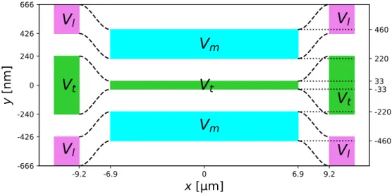
4.5.1 Geometry . . . 48
4.5.2 Self-consistent electrostatic potential . . . 49
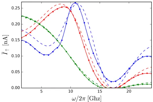
4.5.3 Dc and ac characterization . . . 53
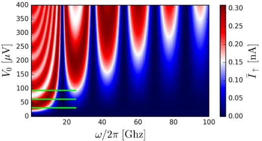
4.5.4 Rectification spectroscopy . . . 54
4.6 Discussion and conclusion . . . 57
5 Josephson junctions in electronic circuits 58 5.1 Introduction to Superconductivity . . . 58
5.1.1 A numerical model of superconductivity . . . 59
5.1.2 Band structure . . . 61
5.1.3 Andreev reflection . . . 62
5.1.4 Superconducting phase . . . 62
5.2 The Josephson junction. . . 63
5.2.1 Ac properties of Josephson junctions . . . 63
5.2.2 Dc properties of Josephson junctions . . . 64
5.2.3 Numerical model of Josephson junctions . . . 65
5.3 Simulation inside electronic environments . . . 67
5.3.1 The RCJ model . . . 67
5.3.2 Results for the RC model . . . 67
5.3.3 Time-dependent RCJ simulation . . . 68
5.3.4 Results for the RLC model . . . 69
5.3.5 Time-dependent RLCJ simulation . . . 71
5.3.6 Short pulse excitation of Josephson junctions . . . 73
5.3.7 Short pulse excitation in RC environment . . . 75
5.4 Topological junction . . . 76
5.4.1 Topological superconductor . . . 76
5.4.2 Majorana bound states . . . 77
5.4.3 Majorana junction inside an RLC resonator . . . 79
6 On the simulation of decoherence 82
6.1 Simulating shot noise . . . 83
6.1.1 Definition of shot noise . . . 83
6.1.2 Model for current noise . . . 83
6.1.3 The stationary case . . . 84
6.1.4 The time-dependent case . . . 85
6.2 Simulating decoherence . . . 86
6.2.1 Density matrix formalism . . . 86
6.2.2 Definition of decoherence . . . 87
6.2.3 From Lindblad to Monte-Carlo . . . 88
6.2.4 Expectation value of observables. . . 89
6.2.5 Non-Hermitian Wick’s theorem . . . 90
6.3 Application to a toy model . . . 92
6.4 Diagrammatic approachs . . . 94
6.5 Conclusion . . . 95
7 Conclusion 96
8 Conclusion en fran¸cais 98
Bibliography 99
Chapter 1
Introduction
In matter, the electric current is produced by the movement of fundamental particles, electrons. Electrons behave according to the laws of quantum mechanics, where they are described by wave packets. The behavior of the wave is disturbed by all the defects of the surrounding matter. The distance at which the electron maintains a wave packet behavior is called coherence length. At room temperature, the coherence length is a few nanometers. In this condition, the wave properties cannot be probed. At cryogenic temperatures, below < 1K, the coherence length can be increased up to a few microm-eters and be accessible to experiments. On the other hand, modern manufacturing technology makes it possible to design electronic circuits with characteristics of a few tenths of a nanometre. It is possible to build experiments where electrons maintain their wave packet behavior throughout a complete electronic circuit. We will call them quantum circuits and the study of this type of circuit is called quantum transport.
The quantum circuits are connected to the macroscopic world by classical electron-ics. This classic electronics is necessary to probe and manipulate the behavior in the circuits by applying different bias voltages. Recent experiments have made it possi-ble to apply a bias voltage that varies rapidly by comparison to the time scale of the electron’s propagation in quantum circuits. This allows us to probe more deeply the characteristics of the quantum circuit, this domain is called time-dependent quantum transport. All connected conventional electronics also change the behavior of quantum circuits. In general, we define by electronic environment everything that is not in the quantum circuit but influences it. Another type of environment is given by Coulomb’s interaction with the electrons of the surrounding environment. The Coulomb interac-tion between electrons is part of the quantum picture. Given the high electron density present in matter, the effect of interaction can often be aggregated by a mean-field theory and considered as a classical interaction, falling into the electronic environment.
The objective of this thesis is to develop theoretical and numerical tools to manage time-dependent quantum transport in quantum circuits by taking into account inter-action with the environment. Recent numerical tools have already been developed to simulate different types of time-dependent quantum circuits [1;2], but the environment was absent from these analyses. This work focuses both on improving these methods and adapting them to take account of the environment. The first part of the introduc-tion provides a general introducintroduc-tion to the field of quantum transport. In the second part, we study the emerging field of time-dependent quantum transport. In the last part, we show the importance of taking into account the electronic environment.
1.1
Mesoscopic quantum electronics
In the absence of external constraint, electrons move in the 3 directions of space. It is difficult to design experiments under these conditions. An important step in building quantum transport experiments has been to reduce the dimensionality of the problem by reducing the movement of electrons in one or two directions. An electron behaves like a wave packet, the characteristic length of variation of the wave packet is given by the Fermi wavelength [3]. The problem can be considered constrained in one direction when the length of freedom along that direction is less than the Fermi wavelength. In a metal, the wavelength of Fermi is in the order of a few angstroms, which is tiny and makes constriction very difficult.
An important step was taken in the 1990s with the use of semiconductors instead of metal. An emblematic example is the two-dimensional electronic gas at the interface of a GaAs/AlGaAs heterostructure. The balance between the Fermi level of the two materials leads to the creation of a small electric field at the interface. This electric field opens a conduction channel in the semiconductor but located at the interface. The electrons are forced to move in the 2D plane of the interface, called 2D electron gas (2DEG). Dimensionality can be further reduced by using voltage gates, metal conduc-tors placed near the 2DEG. The potential of the gates are detected by the electron in the 2DEG, if the potential induced by the conductor is stronger than that one created by the small electric field at the interface, the conduction channel disappears near the conductor. A complete quantum circuit can be created by designing the voltage grid on top of a 2DEG. An example of a Mach-Zehnder interferometer on a 2DEG is shown in Fig. 1.1. The electron gas is situated in a plane parallel to the view, it is constrained by the geometry of the gates shown in the photo.
Figure 1.1: Scanning electron microscope image of the Mach-Zehnder interferometer on a 2DEG, the figure is from Ref. [4]. In grey, blue, and red are metal grids used to constrain the 2DEG situated 140 nm below the surfaces. The white squares represent the ohmic contacts connecting the circuit to the macroscopic world.
1.2
Time-dependent experiments
In a 2DEG, electrons at the Fermi level move at a typical speed of 104to 105 m/s [5]. For
a circuit a few micrometers long, the associated propagation frequency in the circuit is about a few GHz. All voltage variations imposed on the circuit with a frequency greater than the Ghz put the system in a time-dependent state.
The first experiments in the field began with the works of Tien and Gordon [6] in the 1960s. They show that an alternating bias voltage changes the direct current flowing in a circuit, only possible for a circuit in a time-dependent regime. Since then, the field has evolved in many directions, one of the main sources of interest is the construction of a single-electron source. One of the objectives is to reproduce quantum optics experiments with electrons. This field is sometimes called electronic quantum optics. The application of a short bias voltage pulse induces a pulse of current propagating in a 2DEG. The pulse carries a total charge. For a very short pulse, this charge can be reduced to correspond to the charge of a single electron e− [7]. This method is difficult to realize experimentally, but there are other experimental methods to produce single electron sources. In [8], the authors use a quantum dot connected to a conductor via a tunnel barrier in a 2DEG. The electron emission is triggered by the application of a potential step that compensates for the charging energy of the quantum dot. This type of source was used for an electronic experiments of Hanbury-Brown and Twiss [9] or to perform an electronic experiments of Hong-Ou-Mandel [9;10]. Another method uses surface acoustic waves to generate a confinement potential that
propagates and transports individual electrons from a quantum dot to the rest of the circuit. [11; 12].
a.
b.
Figure 1.2: In panel (a.) is a scanning electron microscope image of a Al/Al2Ox/Al
Josephson junction from Ref. [13]. In panel (b.) a transverse diagram of the junction. Aluminum is superconducting at T < 1.2K while the oxide remains metallic at this temperature.
In addition to 2DEG, another very important phenomenon of the time-dependent domain is the Josephson ac effect [14]. 2DGEs and Josephson junctions are based on two different physics. Nevertheless, both can be described by the quantum trans-port theory. A junction consists of two superconductors connected together by a non-superconductive material, Fig.1.2 shows a standard Aluminum/Oxyde/Aluminum junction. Under the application of a constant bias voltage between the two supercon-ductors, an alternating current with a frequency of 2eV /h appears. This oscillation called the ac Josephson effect makes a Josephson junction a highly non-linear elec-tronic component. The most spectacular applications are those that involve inserting a Josephson junction into a conventional electronic circuit to break the linearity of conventional electronics.
1.3
Electronic environments
Many different properties can be obtained by modifying the arrangement of the Joseph-son junctions in an electronic circuit. By coupling two junctions in parallel, we create a loop called Superconducting Quantum Interference Device (SQUID) [15]. A magnetic flux passing through the loop modifies the phase of the electrons in the circuit, the current in the circuit is very sensitive to this phase. On the one hand, a SQUID will act as a sensitive magnetic detector, up to 10−18T, its small scale of a few µm makes it an appropriate tool to probe the magnetic fluxes generated by another electronic circuit. By imposing the magnetic flux inside the loop, we change the behavior of the SQUID as an electronic component. On the other hand, when the two junctions have different energies, the SQUID acts as a tunable Josephson junction.
The construction of superconducting qubits is another application that has been the subject of many recent developments. A qubit is a two-levels quantum system, building an efficient qubit is the basis of quantum computing [16]. With a classical capacitor and inductance, we can create a harmonic oscillator with infinitly many discrete quantum levels. By replacing one of the components with a non-linear Josephson junction, the harmonic oscillator is distorted and the first two levels can be almost isolated from the other levels, creating a qubit. There are multiple possible architectures for a supercon-ducting qubit, fluxonium [17], xmon [18], quantronium [19]. The most famous type is probably the transmon [20], it has attracted the interest of large private companies [21], and it is at the root of recent breakthroughs in the manipulation of the qubit network [22].
1.4
Summary of the thesis
This thesis focuses on the simulation and understanding of quantum transport at the nanoscale, the study of the properties of electrons at low temperatures < 1K and at small scale ∼ µm. This field has existed for decades, but it continues to grow rapidly. Many analytical developments are possible to understand quantum transport [23]. The theory of quantum mechanics is complex, and to obtain analytical results, many hy-potheses are needed to simplify the problem. On the contrary, quantum transport experiments are becoming more and more complex, and numerical tools seem very useful for understanding. Recently, effective simulation tools have been developed as the open software library for the computation of equilibrium quantum transport called Kwant [24]. More recently, our group has also developed algorithms to calculate time-dependent quantum transport [1; 25].
the inclusion of environmental effects in the simulations for a more realistic description of experiments. The effect of the electronic environments surrounding quantum circuits can be broken down into three main factors. First, there is the Coulomb interaction between conduction electrons, the grids and the surrounding material. This physics is already developed by Pacome Armagnat [26] in the context of equilibrium transport. We use this tool to simulate time-dependent quantum transport. Secondly, there is the classical electronic consisting of resistances, capacitors and classical impedances elec-trically connected to the quantum circuit. The whole forms a single electrical circuit where the elements are interdependent, as the quantum part cannot be treated sepa-rately from the rest of the circuit. Finally, we study the effect of a circuit coupled at the quantum level with its environment, also called decoherence. The objective is to model the stochastic phenomena related to quantum noise as well as those caused by the effect of measurement.
Chapter
3
, Simulating time-dependent quantum transport
This chapter begins with the theoretical basis of the simulation of time-dependent quan-tum transport. It shows how to obtain the formalism of wave functions from Green’s famous function formalism. Wave function formalism allows numerical simulations much faster than the standard Non-Equilibrium Green (NEGF) function formalism. This part also completes the demonstration already developed in Ref. [1]. The second part of this chapter is devoted to the numerical tools needed for simulations. Even after the simplification of wave function formalism, a time-based simulation can require hundreds of CPUs for days. In order to simplify calculation costs while maintaining controllable accuracy, many numerical problems must be solved. We give a general description of the solutions used to obtain an efficient parallel simulation algorithm. Finally, we show how to easily include a classical environment in the simulations.Chapter
4
, Spectroscopy of flying qubit
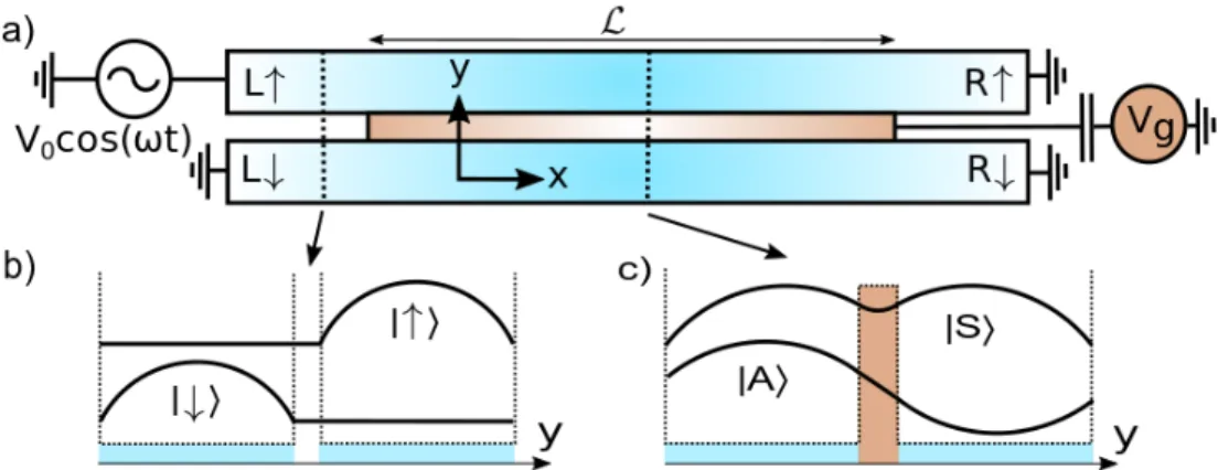
Chapter 4 studies a Mach-Zehnder electronic interferometer and proposes a spectro-scopic technique to probe the internal properties of the interferometer. A 2D electronic gas can be confined with grids to create two parallel conduction channels isolated from each other. An electron can be in a state of superposition on both channels. This superposition propagates along with the pair of channels, creating a flying qubit. Qubit manipulation is done by lowering the barrier between the channels. This allows electrons to tunnel between the two channels. Such geometry creates a Mach-Zehnder electronic interferometer. The first part of the chapter is devoted to understanding a simple
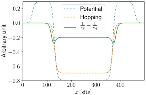
in-terferometer model subjected to a sinusoidal polarization voltage. We compare three models. One uses the time-dependent simulation technique of chapter3, another uses a time-based Floquet formalism, and the latter is a result based on analytical calcula-tions. Combining these results, we propose a method to probe the intrinsic property of the Mach-Zehnder by performing dc measurements accessible to current experiments. The shape of the potential seen by electrons is crucial to understanding interferome-ters. In the second part, we solve the electrostatic problem of the self-consistent Poisson equation to obtain a realistic potential for the quantum circuit. We prove the resilience of our spectroscopy method in the case of a realistic potential at finite temperatures.
Chapter
5
, Josephson junctions in electronic circuits
The chapter5 is devoted to understanding the Josephson junction placed in a conven-tional electronic circuit.
The first part of the chapter reviews superconductivity and existing methods for sim-ulating superconductivity. We apply these methods to the simulation of an environment-free Josephson junction in the time-dependent regime. We quantitatively recover the analytical predictions of the Josephson AC effect and direct current under a constant bias voltage. In the second part, we insert the Josephson junction into different types of conventional circuits, and we use our new self-consistent algorithm, presented in chapter 3, to perform self-consistent simulations over time. The first application is a junction inside an RC circuit where we retrieve the well-known experimental results. The sec-ond application is a junction inside an RLC resonator circuit. We show a qualitative effect resulting from the self-consistent simulation that is not provided by conventional models for such a circuit. Third, we show that an environment-free Josephson junction biased by a short voltage pulse produces an infinite flow of current pulses. We show how the infinite train of pulses degrades in the presence of a dissipative environment. In the last part, we study a model of a topological Josephson junction that presents a Majorana bound state. We study the time-dependent properties of the topological junction. One of the key characteristics of topological junction is the 4π-periodicity of the current-phase relationship. We show how to probe the periodicity with an RLC cir-cuit experimentally, and how the application of a voltage can destroy the 4π-periodicity limiting its observation.
Chapter
6
, On the simulation of decoherence
The last chapter examines different methods for integrating decoherence into a time-dependent simulation. This chapter is part of an ongoing effort to treat the decoherence.
We do not claim to solve the problem in this thesis, but we do open up interesting possibilities for future developments. In the first part, we examine the possibility to recover the statistical properties of the shot noise by using the wave function formalism. In the second part, we study a general decoherence model, the Lindblad equation. The initial model requires exponential computing power, depending on the size of the system. The purpose of this part was to reduce the complexity of the problem to a polynomial problem, accessible to numerical simulation. We demonstrate several possible leads. We develop one possibility into a algorithm. The result is still too slow for an efficient calculation but opens the door to future developments.
Chapter 2
Introduction en fran¸
cais
Dans la mati`ere, le courant ´electrique est produit par le mouvement de particules fonda-mentales, les ´electrons. Les ´electrons se comportent selon les lois de la m´ecanique quan-tique, o`u ils sont d´ecrits par des paquets d’ondes. Le comportement de l’onde est per-turb´e par tous les d´efauts de la mati`ere environnante. La distance `a laquelle l’´electron maintient un comportement de paquet d’ondes est appel´ee longueur de coh´erence. `A temp´erature ambiante, la longueur de coh´erence est de quelques nanom`etres. Dans cette condition, les propri´et´es de l’onde ne peuvent pas ˆetre sond´es. `A des temp´eratures cryog´eniques, inf´erieures `a < 1K, la longueur de coh´erence peut ˆetre augment´ee jusqu’`a quelques microm`etres et ˆetre accessible aux exp´eriences. D’autre part, la technologie de fabrication moderne permet de concevoir des circuits ´electroniques ayant des car-act´eristiques de quelques dixi`emes de nanom`etre. Il est possible de construire des exp´eriences o`u les ´electrons maintiennent leur comportement de paquet d’ondes dans tout un circuit ´electronique. Nous les appellerons des circuits quantiques et l’´etude de ce type de circuit est appel´ee transport quantique.
Les circuits quantiques sont reli´es au monde macroscopique par l’´electronique clas-sique. Cette ´electronique classique est n´ecessaire pour sonder et manipuler le comporte-ment dans les circuits en appliquant diff´erentes tensions de polarisation. Des exp´eriences r´ecentes ont permis d’appliquer une tension de polarisation qui varie rapidement par rapport `a l’´echelle de temps de la propagation de l’´electron dans les circuits quan-tiques. Cela nous permet de sonder plus profond´ement les caract´eristiques du circuit quantique, ce domaine est appel´e transport quantique d´ependant du temps. Tous les appareils ´electroniques conventionnels connect´es modifient ´egalement le comportement des circuits quantiques. En g´en´eral, nous d´efinissons par environnement ´electronique tout ce qui n’est pas dans le circuit quantique mais qui l’influence. Un autre type d’environnement est donn´e par l’interaction de Coulomb avec les ´electrons du milieu
environnant. L’interaction de Coulomb entre les ´electrons fait partie de l’image quan-tique. Etant donn´´ e la forte densit´e d’´electrons pr´esente dans la mati`ere, l’effet de l’interaction peut souvent ˆetre agr´eg´e par une th´eorie du champ moyen et consid´er´e comme une interaction classique, tombant dans l’environnement ´electronique.
L’objectif de cette th`ese est de d´evelopper des outils th´eoriques et num´eriques pour g´erer le transport quantique d´ependant du temps dans les circuits quantiques en prenant en compte l’interaction avec l’environnement. Des outils num´eriques r´ecents ont d´ej`a ´et´e d´evelopp´es pour simuler diff´erents types de circuits quantiques d´ependant du temps [1; 2], mais l’environnement ´etait absent de ces analyses. Ce travail se concentre `a la fois sur l’am´elioration de ces m´ethodes et sur leur adaptation pour tenir compte de l’environnement. La premi`ere partie de l’introduction fournit une introduction g´en´erale au domaine du transport quantique. Dans la deuxi`eme partie, nous ´etudions le domaine ´emergent du transport quantique d´ependant du temps. Dans la derni`ere partie, nous montrons l’importance de la prise en compte de l’environnement ´electronique.
2.1
L’´
electronique quantique m´
esocopique
En l’absence de contrainte ext´erieure, les ´electrons se d´eplacent dans les 3 directions de l’espace. Il est difficile de concevoir des exp´eriences dans ces conditions. Une ´etape importante dans la construction d’exp´eriences de transport quantique a ´et´e de r´eduire la dimensionnalit´e du probl`eme en r´eduisant le mouvement des ´electrons dans une ou deux directions. Un ´electron se comporte comme un paquet d’ondes, la longueur de variation caract´eristique du paquet d’ondes est donn´ee par la longueur d’onde de Fermi [3]. Le probl`eme peut ˆetre consid´er´e comme limit´e `a une direction lorsque la longueur de libert´e dans cette direction est inf´erieure `a la longueur d’onde de Fermi. Dans un m´etal, la longueur d’onde de Fermi est de l’ordre de quelques angstr¨oms, ce qui est minuscule et rend la constriction tr`es difficile.
Un pas important a ´et´e franchi dans les ann´ees 1990 avec l’utilisation de semi-conducteurs `a la place du m´etal. Un exemple embl´ematique est le gaz ´electronique bidimensionnel `a l’interface d’une h´et´erostructure GaAs/AlGaAs. L’´equilibre entre le niveau de Fermi des deux mat´eriaux conduit `a la cr´eation d’un petit champ ´electrique `a l’interface. Ce champ ´electrique ouvre un canal de conduction dans le semi-conducteur mais situ´e `a l’interface. Les ´electrons sont forc´es de se d´eplacer dans le plan 2D de l’interface, appel´e gaz d’´electrons 2D (2DEG). La dimensionnalit´e peut ˆetre encore r´eduite en utilisant des grilles de tension, des conducteurs m´etalliques plac´es pr`es du 2DEG. Le potentiel des grilles est d´etect´e par l’´electron dans le 2DEG, si le potentiel induit par les grilles est plus fort que celui cr´e´e par le petit champ ´electrique `a l’interface, le canal de conduction disparaˆıt pr`es du conducteur. Un circuit quantique complet
peut ˆetre cr´e´e en concevant la grille de tension au-dessus d’un 2DEG. Un exemple d’interf´erom`etre Mach-Zehnder sur un 2DEG est pr´esent´e sur la figure 1.1. Le gaz d’´electrons est situ´e dans un plan parall`ele `a la vue, il est contraint par la g´eom´etrie des grilles montr´ees sur la photo.
Figure 2.1: Image au microscope ´electronique `a balayage de l’interf´erom`etre Mach-Zehnder sur un 2DEG, la figure est de [4]. En gris, bleu et rouge sont des grilles m´etalliques utilis´ees pour contraindre le 2DEG sutu´e `a 140 nm sous les surfaces. Les carr´es blancs repr´esentent les contacts ohmiques se connectant au monde macro-scopique.
2.2
Les exp´
eriences d´
ependentes du temps
Dans un 2DEG, les ´electrons au niveau de Fermi se d´eplacent `a une vitesse typique de 104 `a 105 m/s [5]. Pour un circuit de quelques microm`etres de long, la fr´equence de
propagation associ´ee dans le circuit est d’environ quelques GHz. Toutes les variations de tension impos´ees au circuit avec une fr´equence sup´erieure au Ghz mettent le syst`eme dans un ´etat d´ependant du temps.
Les premi`eres exp´eriences dans ce domaine ont commenc´e avec les travaux de Tien et Gordon [6] dans les ann´ees 1960. Ils montrent qu’une tension de polarisation alter-native modifie le courant continu circulant dans un circuit, ce qui n’est possible que pour un circuit en r´egime d´ependant du temps. Depuis lors, le domaine a ´evolu´e dans de nombreuses directions, l’une des principales sources d’int´erˆet ´etant la construction d’une source d’´electrons unique. L’un des objectifs est de reproduire des exp´eriences d’optique quantique avec des ´electrons. Ce domaine est parfois appel´e optique quan-tique ´electronique. L’application d’une courte impulsion de tension de polarisation
induit une impulsion de courant se propageant dans un 2DEG. L’impulsion porte une charge totale. Pour une impulsion tr`es courte, cette charge peut ˆetre r´eduite pour cor-respondre `a la charge d’un seul ´electron e− [7]. Cette m´ethode est difficile `a r´ealiser exp´erimentalement, mais il existe d’autres m´ethodes exp´erimentales pour produire des sources d’´electrons uniques. Dans [8], les auteurs utilisent un point quantique connect´e `
a un conducteur par une barri`ere tunnel dans un 2DEG. L’´emission d’´electrons est d´eclench´ee par l’application d’un saut de potentiel qui compense l’´energie de charge du point quantique. Ce type de source a ´et´e utilis´e pour des exp´eriences ´electroniques de Hanbury-Brown et Twiss [9] ou pour r´ealiser des exp´eriences ´electroniques de Hong-Ou-Mandel [9;10]. Une autre m´ethode utilise les ondes acoustiques de surface pour g´en´erer un potentiel confinement qui se propage et qui transporte les ´electrons individuels d’un point quantique au reste du circuit [11;12].
a.
b.
Figure 2.2: Dans le panneau (a.) se trouve une image au microscope ´electronique `a balayage d’une junction Josephson Al/Al2Ox/Al prise de Ref. [13]. Dans le panneau
(b.) un diagramme transversal de la jonction. L’aluminium est supraconducteur `a T < 1.2K alors que l’oxyde reste m´etallique `a cette temp´erature.
Outre le 2DEG, un autre ph´enom`ene tr`es important du domaine temporel est l’effet Josephson ac [14]. Les 2DGE et les jonctions de Josephson sont bas´ees sur deux physiques diff´erentes. N´eanmoins, les deux peuvent ˆetre d´ecrites par la th´eorie du
transport quantique. Une jonction est constitu´ee de deux supraconducteurs reli´es entre eux par un mat´eriau non supraconducteur. La figure 1.2 montre une jonction stan-dard Aluminium/Oxyde/Aluminium. Sous l’application d’une tension de polarisation constante entre les deux supraconducteurs, un courant alternatif d’une fr´equence de 2eV /h apparaˆıt. Cette oscillation, appel´ee effet Josephson alternatif, fait de la jonction Josephson un composant ´electronique hautement non lin´eaire. Les applications les plus spectaculaires sont celles qui consistent `a ins´erer une jonction Josephson dans un circuit ´electronique conventionnel pour rompre la lin´earit´e de l’´electronique conventionnelle.
2.3
Les environnements ´
electroniques
De nombreuses propri´et´es diff´erentes peuvent ˆetre obtenues en modifiant la disposition des jonctions Josephson dans un circuit ´electronique. En couplant deux jonctions en parall`ele, on cr´ee une boucle appel´ee dispositif d’interf´erence quantique supraconducteur (SQUID) [15]. Un flux magn´etique traversant la boucle modifie la phase des ´electrons dans le circuit, le courant dans le circuit est tr`es sensible `a cette phase. D’une part, un SQUID agira comme un d´etecteur magn´etique sensible, jusqu’`a 10−18T, sa petite ´echelle de quelques µm en fait un outil appropri´e pour sonder les flux magn´etiques g´en´er´es par un autre circuit ´electronique. En imposant le flux magn´etique `a l’int´erieur de la boucle, nous modifions le comportement du SQUID en tant que composant ´electronique. D’autre part, lorsque les deux jonctions ont des ´energies diff´erentes, le SQUID agit comme une jonction Josephson accordable.
La construction de qubits supraconducteurs est une autre application qui a fait l’objet de nombreux d´eveloppements r´ecents. Un qubit est un syst`eme quantique `a deux niveaux, la construction d’un qubit efficace est la base de l’informatique quan-tique [16]. Avec un condensateur et une inductance classiques, nous pouvons cr´eer un oscillateur harmonique avec une infinit´e de niveaux quantiques discrets. En rempla¸cant l’un des composants par une jonction Josephson non lin´eaire, l’oscillateur harmonique est d´eform´e et les deux premiers niveaux peuvent ˆetre presque isol´es des autres niveaux, cr´eant ainsi un qubit. Il existe de multiples architectures possibles pour un qubit supra-conducteur, fluxonium [17], xmon [18], quantronium [19]. Le type le plus connu est probablement le transmon [20], il a suscit´e l’int´erˆet de grandes entreprises priv´ees [21], et il est `a l’origine de r´ecentes perc´ees dans la manipulation du r´eseau de qubit [22].
2.4
R´
esum´
e de la th`
ese
Cette th`ese porte sur la simulation et la compr´ehension du transport quantique `a l’´echelle nanom´etrique, l’´etude des propri´et´es des ´electrons `a basse temp´erature < 1K et `a petite ´echelle ∼ µm. Ce domaine existe depuis des d´ecennies, mais il continue `
a se d´evelopper rapidement. De nombreux d´eveloppements analytiques sont possibles pour comprendre le transport quantique [23]. La th´eorie de la m´ecanique quantique est complexe, et pour obtenir des r´esultats analytiques, de nombreuses hypoth`eses sont n´ecessaires pour simplifier le probl`eme. Au contraire, les exp´eriences de trans-port quantique deviennent de plus en plus complexes, et les outils num´eriques semblent tr`es utiles pour la compr´ehension. R´ecemment, des outils de simulation efficaces ont ´et´e d´evelopp´es comme la biblioth`eque logicielle ouverte pour le calcul du transport quantique `a l’´equilibre appel´ee Kwant [24]. Plus r´ecemment, notre groupe a ´egalement d´evelopp´e des algorithmes pour calculer le transport quantique en fonction du temps [1; 25].
Le but de cette th`ese est d’am´eliorer leur travail `a la fois avec une plus grande ef-ficacit´e et avec l’inclusion des effets de l’environment dans les simulations pour une description plus r´ealiste des exp´eriences. L’effet des environnements ´electroniques entourant les circuits quantiques peut ˆetre d´ecompos´e en trois facteurs principaux. Premi`erement, il y a l’interaction de Coulomb entre les ´electrons de conduction, les grilles et le mat´eriau environnant. Cette physique est d´ej`a d´evelopp´ee par Pacome Armagnat [26] dans le contexte du transport `a l’´equilibre. Nous utilisons cet outil pour simuler le transport quantique d´ependant du temps. Ensuite, il y a l’´electronique classique compos´ee de r´esistance, de condensateur et d’imp´edance classique connect´es ´electriquement au circuit quantique. L’ensemble forme un circuit ´electrique unique o`u les ´el´ements sont interd´ependants, car la partie quantique ne peut ˆetre trait´ee s´epar´ement du reste du circuit. Enfin, nous ´etudions l’effet d’un circuit coupl´e au niveau quantique avec son environnement, ´egalement appel´e d´ecoh´erence. L’objectif est de mod´eliser les ph´enom`enes stochastiques li´es au bruit quantique ainsi que ceux caus´es par l’effet de mesure.
Chapitre
3
, Simulation du transport quantique d´
ependant du
temps
Ce chapitre commence par les bases th´eoriques de la simulation du transport quantique d´ependant du temps. Il montre comment obtenir le formalisme des fonctions d’onde `a partir du fameux formalisme de fonction de Green. Le formalisme des fonctions d’onde permet des simulations num´eriques beaucoup plus rapides que le formalisme standard
des fonctions de Green hors-´equilibre (NEGF). Cette partie compl`ete ´egalement la d´emonstration d´ej`a d´evelopp´ee dans Ref. [1]. La deuxi`eme partie de ce chapitre est consacr´ee aux outils num´eriques n´ecessaires aux simulations. Mˆeme apr`es la simpli-fication du formalisme des fonctions d’onde, une simulation bas´ee sur le temps peut n´ecessiter des centaines de CPU pendant plusieurs jours. Afin de simplifier les coˆuts de calcul tout en maintenant une pr´ecision contrˆolable, de nombreux probl`emes num´eriques doivent ˆetre r´esolus. Nous donnons une description g´en´erale des solutions utilis´ees pour obtenir un algorithme de simulation parall`ele efficace. Enfin, nous montrons comment inclure facilement un environnement classique dans les simulations.
Chapitre
4
, Spectroscopie du qubit volant
Le chapitre4´etudie un interf´erom`etre ´electronique Mach-Zehnder et propose une tech-nique spectroscopique pour sonder les propri´et´es internes de l’interf´erom`etre. Un gaz ´electronique 2D peut ˆetre confin´e avec des grilles pour cr´eer deux canaux de conduction parall`eles isol´es l’un de l’autre. Un ´electron peut ˆetre dans un ´etat de superposition entre les deux canaux. Cette superposition se propage en mˆeme temps que la paire de canaux, cr´eant un qubit volant. La manipulation du qubit se fait en abaissant la barri`ere entre les canaux. Cela permet aux ´electrons de creuser un tunnel entre les deux canaux. Une telle g´eom´etrie cr´ee un interf´erom`etre ´electronique Mach-Zehnder. La premi`ere partie du chapitre est consacr´ee `a la compr´ehension d’un mod`ele d’interf´erom`etre sim-ple soumis `a une tension de polarisation sinuso¨ıdale. Nous comparons trois mod`eles. L’un utilise la technique de simulation d´ependant du temps du chapitre 3, un autre utilise un formalisme de Floquet bas´e sur le temps, et le dernier est un r´esultat bas´e sur des calculs analytiques. En combinant ces r´esultats, nous proposons une m´ethode pour sonder la propri´et´e intrins`eque du Mach-Zehnder en effectuant des mesures en courant continu accessibles aux exp´eriences actuelles. La forme du potentiel vu par les ´electrons est cruciale pour comprendre les interf´erom`etres. Dans la deuxi`eme partie, nous r´esolvons le probl`eme ´electrostatique de l’´equation de Poisson autoconsistante afin d’obtenir un potentiel r´ealiste pour le circuit quantique. Nous prouvons la r´esilience de notre m´ethode de spectroscopie dans le cas d’un potentiel r´ealiste `a des temp´eratures finies.
Chapitre
5
, Jonctions Josephson dans des circuits ´
electroniques
Le chapitre 5est consacr´e `a la compr´ehension de la jonction Josephson plac´ee dans un circuit ´electronique classique. La premi`ere partie du chapitre passe en revue la supra-conductivit´e et les m´ethodes existantes de simulation de la supraconductivit´e. Nousappliquons ces m´ethodes `a la simulation d’une jonction Josephson sans environnement dans le r´egime d´ependant du temps. Nous r´ecup´erons quantitativement les pr´edictions analytiques de l’effet Josephson AC et du courant continu sous une tension de polar-isation constante. Dans la deuxi`eme partie, nous ins´erons la jonction Josephson dans diff´erents types de circuits classiques et nous utilisons notre nouvel algorithme autocon-sistant, pr´esent´e au chapitre 3, pour effectuer des simulations autoconsistantes dans le temps. La premi`ere application est une jonction `a l’int´erieur d’un circuit RC o`u nous r´ecup´erons les r´esultats exp´erimentaux bien connus. La deuxi`eme application est une jonction `a l’int´erieur d’un circuit r´esonateur RLC. Nous montrons un effet qualitatif r´esultant de la simulation auto-coh´erente qui n’est pas fourni par les mod`eles conven-tionnels pour un tel circuit. Troisi`emement, nous montrons qu’une jonction Josephson sans environnement, polaris´ee par une courte impulsion de tension, produit un flux infini d’impulsions de courant. Nous montrons comment le train infini d’impulsions se d´egrade en pr´esence d’un environnement dissipatif. Dans la derni`ere partie, nous ´etudions un mod`ele de jonction Josephson topologique qui pr´esente un ´etat li´e de Ma-jorana. Nous ´etudions les propri´et´es de la jonction topologique qui d´ependent du temps. L’une des caract´eristiques cl´es de la jonction topologique est la p´eriodicit´e de la relation entre le courant et la phase. Nous montrons comment sonder exp´erimentalement la 4π-p´eriodicit´e avec un circuit RLC, et comment l’application d’une tension peut d´etruire la p´eriodicit´e de 4π limitant son observation.
Chapitre
6
, De la simulation de la d´
ecoh´
erence
Le dernier chapitre examine les diff´erentes m´ethodes d’int´egration de la d´ecoh´erence dans une simulation en fonction du temps. Ce chapitre s’inscrit dans le cadre d’un effort continu pour traiter la d´ecoh´erence. Nous ne pr´etendons pas r´esoudre le probl`eme dans cette th`ese, mais nous ouvrons des possibilit´es int´eressantes pour des d´eveloppements futurs. Dans la premi`ere partie, nous examinons la possibilit´e de r´ecup´erer les propri´et´es statistiques du bruit de grenaille en utilisant le formalisme de la fonction d’onde.
Dans la deuxi`eme partie, nous ´etudions un mod`ele g´en´eral de d´ecoh´erence, l’´equation de Lindblad. Le mod`ele initial n´ecessite une puissance de calcul exponentielle, en fonc-tion de la taille du syst`eme. L’objectif de cette partie ´etait de r´eduire la complexit´e du probl`eme `a un probl`eme polynomial, accessible `a la simulation num´erique. Nous d´emontrons plusieurs pistes possibles. Nous d´eveloppons une possibilit´e en un algo-rithme. Le r´esultat est encore trop lent pour un calcul efficace mais ouvre la porte `a des d´eveloppements futurs.
Chapter 3
Simulating time-dependent
quantum transport
3.1
Green’s function formalism of time-dependent
problem
The objective of this chapter is to simulate quantum nanoelectronics, the motion of the electron in a condensed matter medium. The starting point is a general description of a quantum system in nanoelectronics. We aim to simulate non-interactive problems defined by a quadratic Hamiltonian, in the tight-binding formalism
ˆ
H =XHij(t)ˆc
†
icˆj, (3.1)
where ˆc†i and ˆci are the creation and annihilation of an electron on the i site. The
Hij matrix is a representation of the Hamiltonian in this operator base. The state of
a quantum system is described by a vector ψ from Hilbert’s space, the Shr¨odinger” equation gives the equation of the system’s motion
i~∂tψ = ˆHψ. (3.2)
The general objective is to simulate a quantum system that can be inserted into a conventional electrical circuit as a multiterminal component. From the point of view of the conventional circuit, a conductor is entirely defined by its statistical properties: voltage, current, temperature and chemical potential. Within the quantum circuit, there are also quantum properties arising from correlations between electrons. To make the transition between the two, we model lead by a semi-infinite system. One end is attached to the quantum system and the other end is at infinity, towards the classical
system. Any quantum correlation disappears during propagation along the infinite lead and only the statistical properties remain. The central region where all the wires are connected is of finite volume, and can have any shape or dimension: 1D, 2D or 3D.
Because of the semi-infinite leads, the global system is infinite in size. This makes direct numerical simulation impossible. The purpose of this section is to simplify the equations into an equivalent finite size system.
...
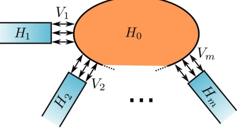
Figure 3.1: System constituted of a scattering region labeled 0 connected to semi-infinite leads 1, . . . , m through couplings elements noted Vi.
3.1.1
Problem modeling
The objective is to reduce the infinite problem to a finite size problem. First, the Hamiltonian in our system is separated in its subsections. There is the dispersion region with a Hamiltonian H0 and there are semi-infinite leads with Hamiltonians Hi∈[1,m].
Leads are connected to the diffusion region by coupling elements Vi∈[1,m] cf Figure3.1.
The Hamiltonian takes the form of
ˆ H = H0 V1 . . . Vm V1† H1 0 .. . . .. Vm† 0 Hm . (3.3)
The formalism of Green’s function applies to our problem where the strength of the coupling elements Vi∈[1,m] between the central region and the lead is treated as the
a perturbative regime. The greater, lesser, time-ordered, anti-ordered, advanced and retarded fermionic Green’s functions are introduced as usual, using the notation of [27] they read G>(x, t, x0, t0) = −i hˆc(x, t)ˆc†(x0, t0)i , G<(x, t, x0, t0) = i hˆc†(x0, t0)ˆc(x, t)i , GT(x, t, x0, t0) = −i hT (ˆc(x, t)ˆc†(x0, t0))i , GT˜(x, t, x0, t0) = −i h ˜T (ˆc(x, t)ˆc†(x0, t0))i , GA(x, t, x0, t0) = −iθ(t0− t) hˆc(x, t)ˆc†(x0, t0)i , GR(x, t, x0, t0) = iθ(t − t0)Dc(x, t)ˆˆ c†(x0, t0)E, (3.4) where ˆc(x, t) and ˆc†(x, t) are the annihilation and creation operators at position x at time t. T and ˜T are the time and anti-time ordering operators. The Dyson relationship of [27] is used to link the different types of Green’s functions together
GT G< G> GT˜ ! = g T g< g> gT˜ ! + g T g< g> gT˜ ! V 0 0 −V ! GT G< G> GT˜ ! . (3.5)
where ˆg notes the Green’s function of the system without V coupling elements. The equation3.5contains all the information necessary to solve the problem. The following sections are devoted to simplifying the equation to obtain a form suitable for numer-ical computation. Green’s functions are related to the physnumer-ical observables thanks to Wick’s theorem. The lesser Green’s function G<(t, t0) is the most suitable to use Wick’s
theorem, so we concentrate our effort on obtaining it.
The time-ordered Green’s functions are expressed as a combination of the other Green’s functions gT = gR+ g< and GT˜ = G<− GA by manipulating the operators in
the equations that define the Green’s functions. These relationships are used with the Dyson equation Eq.3.5 to obtain a closed system of equations for the lower, advanced and retarded Green’s functions
G< = g<+ gRV G<+ g<V GA, GR = gR+ gRV GR,
GA = gA+ gAV GA. (3.6)
3.1.2
Separating regions
GA, GR, and G< contain information about the complete infinite system. Only the
calculations. The idea is to separate the equation for the different regions, the central part and the tracks, in order to isolate a closed formula for Green’s function from the central part. The following demonstration is based on the work of [28] and [29]. We remember the 0 index tags the central region and indexes i ≥ 1 tags the leads. Gij
notes the Green’s function (advanced, delayed or lower) from the region i (x ∈ i) to the region j (x’ ∈ j). Using this notation, the Green’s functions GA, GR, and G< take
the following forms
G∗ = G∗00 G∗01 . . . G∗0m G∗10 G∗11 . . . G∗1m .. . ... . .. ... G∗m0 G∗m1 . . . G∗mm . (3.7)
where G∗ is either GA, GR, or G<. Green’s functions of the system without coupling
(V = 0) are by definition block diagonal
g∗ = g00∗ 0 g∗11 . .. 0 gmm∗ . (3.8)
where g∗ is either gA, gR, or g<. The coupling in this base is by definition
V = 0 V1 . . . Vm V1 .. . 0 Vm . (3.9)
Inserting notations Eq.3.7, Eq.3.8, Eq.3.8 into the Dyson equation Eq.3.6 gives the relations between the Green’s functions of the different regions. For all regions i, j
G<ij = gij<+X kl gikRVklG<lj + X kl gik<VklGAlj, (3.10a) GRij = gijR+X kl gikRVklGRlj, (3.10b) GAij = gijA+X kl gikAVklGAlj. (3.10c)
Here we did nothing but rewrite Eq.3.6using different notations. Now that the indexes of the different regions are explicitly visible, it is easier to separate the regions.
3.1.3
Retarded and advanced Green’s functions
The Eq. 3.10b is a closed formula with only retarded Green’s functions, it is used to obtain an equation of motion for GR
00. The region 0 is separated from the others
GR00 = gR00+X
l
gR00VlGRl0,
∀i ≥ 1, GRi0 = giiRViGR00. (3.11)
The combination of the two equations gives the Dyson equation for the central region only
GR00 = gR00+ g00RΣRGR00, (3.12) where the retarded self-energy of the leads without interactions is defined as
ΣR=X
l
VlgllRVl. (3.13)
The self-energy is defined on the system without interaction, it will be treated in the next section. The equation of motion for the retarded Green’s function is obtained by applying the derivative (i∂t− H0) to the previous equation
(i~∂t− H0(t) − ΣR)GR00= δ(t − t 0
), (3.14)
where we used the property of the Green’s function (i~∂t− H0)g00R = δ(t − t
0).
Equa-tion3.14 provides a differential equation involving GR
00 with a finite spatial extension
and ΣR calculated from the non-interacting system. This equation can be numerically integrated to obtain GR
00(t, t
0) at any time. With a similar demonstration, the problem
for the advanced Green’s function is solved by using Eq.3.10c to obtain
GA00 = gA00+ g00AΣAGA00, (3.15) and the differential equation
(i~∂t− H0(t) − ΣA)GA00= δ(t − t 0
), (3.16)
where ΣA=P
lVlgAllVl is the advanced self-energy.
3.1.4
Lesser Green’s functions
Eq.3.10a is solved to obtain an equation for the lesser Green’s function within the scattering region G<
00. The demonstration is similar to the one used for the retarded
Green’s function. The central region is separated from the other region, from Eq.3.10a
G<00 = g<00+ g00R X l>0 VlG<l0+ g < 00 X l>0 VlGAl0. (3.17)
and ∀i ≥ 1, G<i0 =X kl gikRVklG<l0+ X kl g<ikVklGAl0, GAi0 =X i giiAViGA00. (3.18)
By replacing Eq.3.18 in Eq.3.17 we get
G<00=g00< + gR00ΣRG<00+ g00RΣ<GA00+ g<00ΣAGA00, (3.19) where the lesser self-energy of the leads without interactions is defined by Σ< = V g<V . The previous equality is rewritten as follows
(1 − g00RΣR)G<00 = g00RΣ<GA00+ g00<(1 + ΣAGA00). (3.20) Finally the equation is multiplied to the left by (1 + GR
00ΣR) and results on the retarded
Green’s function of the previous part (Eq.3.12) are used to obtain a simplify form, commonly referred as the Keldysh equation [30],
G<00= GR00Σ<GA00+ (1 + G00RΣR)g00<(1 + ΣAGA00). (3.21)
The left side is G<00 the Green’s function in the central region, it is the quantity we are trying to explicit. The right side decompose into two terms.
The first term is composed with the self-energy Σ< and the Green’s function GR
00
and GA00. The lesser self-energy of the leads is defined by using g00R, the retarded Green’s function of the central region in the absence of coupling to the lead, and without cou-pling the central region is a closed system that can be solved by many methods. The retarded and advanced Green’s functions can be obtain by solving the equation of mo-tion Eq.3.14and Eq.3.16. The numerical calculation of GR
00Σ<GA00 is the main subject
of the article Ref. [1]. All the methods studied in the article Ref. [1] are based on a tight-binding model and gives the same results. The differences lie in the computational costs in both time and memory. The most effective method is the wave function approach, described in the next section. It has a better scaling than the other non-equilibrium Green’s function method, providing the massive acceleration needed to simulate a com-plex system. Simulations were performed up to ∝ 105 sites and 106 times the smallest
time scale of the system.
The second term (1+GR00ΣR)g<(1+ΣAGA00) corresponds to the contribution of bound
states. In the non-interacting case, bound states do not participate in the conduction measured far inside the leads. The term is often neglected for analytical purposes [30], [31]. In numerical simulations, the conduction properties are measured at a finite distance from the scattering region where bound states have not decayed and must be taken into account. For consistency with the first term, the wave function formalism is used to calculate this term.
3.2
The wave function approach
The lesser self-energy is defined by Σ<(t, t0) = V g<(t, t0)V . Hamiltonians of lead are not time-dependent, and g< corresponds to the Green’s function of lead without coupling
to the scattering region. Thus, the lesser self-energy is invariant by translation in time Σ<(t, t0) = Σ<(t − t0). The Fourier decomposition is used to obtain the decomposition into energies Σ<(t − t0) = X l Z dE 2πifle −i ~E(t−t 0) Γl(E), (3.22)
where l labels the leads. The Kernel Γl is diagonalized, in the “dual transverse wave
function” bases, see Ref. [31],
Γm(E) = X α vmαξαEξ † αE. (3.23)
By inserting this decomposition into the Eq.3.21we obtain the lesser Green’s function as an integral over the wave functions
GR00Σ<GA00 =X
α
Z dE
2πifα(E)ψαE(t)ψαE(t
0
)†, (3.24)
with wave functions defined as ψαE(t) =
√
vαEGR00ξαE. The equation of motion for the
wave functions is obtained from the equation of motion of the retarded Green’s function Eq.3.14,
i~∂tψαE = ˆH(t)ψαE +
√ vαe−i
E
~tξαE. (3.25)
The second term of the equation 3.21 is rewritten be using equation Eq.3.12 and 3.15 to obtain (1 + GR00ΣR)g<(1 + ΣAGA00) = G R 00 h (gR)−1g<(gA)−1iGA00. (3.26) The central part of this equation is defined by non-interacting Green’s function of the central region only, we can use the Fourier transform. For a central region with a finite size, the kernel of the Fourier transform is diagonalized into bound state labeled by the index γ, (gR)−1g<(gA)−1(t − t0) = Z dE 2πf0(E)e −i ~E(t−t 0)X γ ξγEξ † γE. (3.27)
The occupation function f0 is the occupation of the scattering region at the initial time
t = −∞. We suppose the occupation in the central region and the occupation in the leads are equal and correspond to a Fermi occupation. This is the case if interaction
processes have occurred far in the past and have coupled bound states to the continuum. The wave functions are recovered with the action of the Green’s function
(1 + GR00ΣR)g<(1 + ΣAGA00) =
X
γ
f0(E)ψγE(t)ψγE(t0)†, (3.28)
where wave functions obey the equation of motion 3.25 by replacing √vαe−
i
~EtξαE by
the its equivalent for bound states e−~iEtξγE,
i~∂tψγE = ˆH(t)ψαE + e−i
E
~tξγE. (3.29)
3.3
An algorithm for time-dependent simulation
Results of the previous section are gathered into the equation G<(t, t0) =X
α
Z dE
2πifα(E)ψαE(t)ψαE(t
0
)†+X
γ
f0(E)ψγE(t)ψγE(t0)†, (3.30)
where γ sum on all propagating modes and γ sum over all bound states. The wave functions of propagating modes follow the equation
i∂tψαE = ˆH(t)ψαE +
√ vαe−
i
~EtξαE, (3.31)
where√vα = 1 for wave functions corresponding to bound states. The combination of
Eq.3.30 and Eq.3.31 is the basis for numerical calculations.
Numerical methods of resolution of this set of equation where already know from Ref. [25]. Unfortunately, the numerical algorithms used were not very accurate and quite costly in terms of computing time. A large part of the thesis consisted in refining the different numerical methods to improve both accuracy and computation time, thus opening the doors to more expensive simulations such as those including the environ-ment. This rather technical section describes the numerical methods used to efficiently solve the equations Eq.3.30 and Eq.3.31.
3.3.1
Search for initial wave functions
The first step is to obtain the initial conditions for the equations of motion, wave functions ψαE(t = 0) for all energies and modes.
The propagative case
The time-dependent perturbation is activated at t ≥ 0. Before the time-dependent perturbation, the wave functions are solutions of the stationary equation derived from Eq.3.31,
[~E − ˆH0− ΣR(E)]ψst =
√
vαξαE, (3.32)
where ˆH0 = ˆH(t ≤ 0) is the Hamiltonian without time-dependent perturbation. There
are many standard techniques available to obtain the solution of this equation. The Kwant package [24] is an open-source quantum transport software whose performance is among the best for this type of problem. The resolution is obtained using a tight-binding model. The quasi-periodicity of the lead allows the semi-infinite equation3.32 to be reduced to a linear system of finite size equations. The result of the algorithm are the numerical values of the wave function at each site. We refer the reader to the website of Kwant [32] for more details.
The bound state case
Bound states are eigenstates of the Hamiltonian that do not propagate in the lead, where they decay exponentially. For a finite size system with a quadratic Hamiltonian
ˆ H0 = X ij hijˆc † iˆcj, (3.33)
where h is a N × N matrix with N the number of sites in the central region. The energies of bound states is given by the eigenvalues of the h matrix and the associated eigenvectors give the values of wave functions.
In the case of a system with semi-infinite lead, direct diagonalization is not possible. The standard method of resolution use the exponential decay of the wave function of bound state in all leads. The semi-infinite lead can be truncated after a sufficient length for the wave function to disappear. The semi-infinite lead is truncated after sufficient time for the wave function to disappear. The resulting finite Hamiltonian can be diagonalized by standard techniques to give an approximation of the wave function, up to the vanishing part. However this poses two problems, one is to estimate the length of decay required. A too short length gives a bad approximation, a too long length gives a too long calculation time. Another problem is that the length of decay can be arbitrarily long, which is usually the case for related states that are close in energy to a propagation mode.
Fortunately a method that doesn’t require truncation is developed in Ref. [33]. They use a technique similar to that used in transportation software to reduce the problem
of an infinite Hamiltonian to the resolution of an equivalent finite size linear system. The algorithm has proven to be robust and as an advantage to be compatible with the Kwant package.
3.3.2
Time evolution of wave functions
The second step is too evolve the initial wave function by using the equations of motion Eq.3.31.
i∂tψαE = ˆH(t)ψαE +
√ vαe−
i
~EtξαE.
For t ≤ 0 there is no time-dependent perturbation, by definition of the stationary initial conditions the solution are trivial
ψαE(t) = e−iEtψαE(0), ∀t ≤ 0. (3.34)
For t > 0 the time-dependent perturbation is turned on, a standard linear differential is obtained which is effectively integrated by the Runge-Kutta methods [34]. However wave-functions are define on an infinite system, inaccessible to numerical resolution. Two properties are used to reduce the size of the simulation to a finite size.
First all the time-dependent perturbation are gathered ˆHt(t) into the central
re-gion. If the time-dependent disturbance is present at a finite number of sites, the central region is defined as encompassing all time-dependent sites. If a time-dependent perturbation V (t) applies to a semi-infinite lead, the wave function ψ and the Hamilto-nian function ˆH are decomposed into the lead part (label l), the diffusion region (label s) and the interface (label sl). In this cases the equation of motion reads as follows
i~∂tψ = ˆHsψs+ ( ˆHl+ V (t))ψl+ ˆHslψ +
√ vαe−
i
~EtξαE. (3.35)
The gauge transformation is applied in the part of the wave function in the lead with ˜ ψl = e−i R V (t) ψl and ˜ψs= ψs i~∂tψ =˜ H(t) ˜ˆ˜ ψ + √ vαe− i ~EtξαE, (3.36) where H = ˆˆ˜ Hs + ˆHl + ˆHslei R
V (t). Now the lead is time-independent and only the
interface with the central region is time-dependent.
For t ≤ the stationary solution and the real solution are the same. For t > 0 the time-dependent perturbation is located only in the central region, and physical signals always have a maximal propagation speed, noted vmax. So at time t the difference
between the stationary wave function and the time-dependent wave function are limited in a region L < t × vmax around the central region. Thus only a finite region around
the central region is useful for numerical simulation. It is done by considering only the difference ψαEd between the extended stationary solution and the time-dependent solution
ψαEd (t) = ˜ψαE(t) − ψαE(0)e
i
~Et. (3.37)
The equation of motion for the difference is obtained by combining the equation of motion of each part,
i∂tψdαE =Hψˆ˜ d
αE + ˆHte−
i
~EtψαE(0), (3.38)
where the Hamiltonian breaks down into time-dependent part and the stationary part ˆ
˜
H =Hˆ˜0+Hˆ˜t.
3.3.3
Absorbing boundary conditions
The size of the system can be further reduced by noting that in most systems, there is no backscatter from the leads to the central region, which means that all the information sent to the leads never returns to the central region. This can be used to truncate the system before the length vmaxtmax. An imaginary potential in leads is a way to
absorb outgoing signals. The basis of the method is developed in Ref. [25] and has been completed by Thomas Kloss. The difficulty is to create an imaginary potential strong enough to absorb the outgoing signals but smooth enough not to create backscatter.
In a semi-infinite periodic lead, any physical signal can be decomposed into a sum of standing wave function
ψ(t) =X
α
Z
dE hψαE|ψ(t)i ψαEe−
i
~Et. (3.39)
To ensure that the signal is correctly absorbed at all times, it is sufficient to verify that the standing wave function of all modes and energies, ψαE, are absorbed by the
imaginary potential. To simplify the calculation of the absorption, we limit ourselves to the case of a 1D lead, with the dimension noted x. The amplitude of the imaginary potential is noted Σ(x), the stationary solution in an imaginary potential is given by the Shr¨odinger equation, in natural units it is read
− i~∂tψαE − iΣψαE = EψαE. (3.40)
The wave function is decomposed into a superposition of incoming and outgoing plane waves

![Figure 4.1: Scanning electron microscope image of the aircraft in flight qubit sample, image from [4]](https://thumb-eu.123doks.com/thumbv2/123doknet/12705837.355840/49.918.201.727.149.352/figure-scanning-electron-microscope-image-aircraft-flight-sample.webp)