Nonlinear Marangoni convection in circular and elliptical cylinders

(1)

HAL Id: hal-01785165

https://hal.archives-ouvertes.fr/hal-01785165

Submitted on 4 May 2018

HAL is a multi-disciplinary open access

archive for the deposit and dissemination of

sci-entific research documents, whether they are

pub-lished or not. The documents may come from

teaching and research institutions in France or

abroad, or from public or private research centers.

L’archive ouverte pluridisciplinaire HAL, est

destinée au dépôt et à la diffusion de documents

scientifiques de niveau recherche, publiés ou non,

émanant des établissements d’enseignement et de

recherche français ou étrangers, des laboratoires

publics ou privés.

Nonlinear Marangoni convection in circular and

elliptical cylinders

Pauline Assemat, Alain Bergeon, Edgar Knobloch

To cite this version:

Pauline Assemat, Alain Bergeon, Edgar Knobloch. Nonlinear Marangoni convection in circular and

elliptical cylinders. Physics of Fluids, American Institute of Physics, 2007, vol. 19 (n° 10), pp. 1-17.

�10.1063/1.2771566�. �hal-01785165�

(2)

To cite this version :

Assemat, Pauline

and Bergeon, Alain

and Knobloch, Edgar Nonlinear

Marangoni convection in circular and elliptical cylinders.

(2007) Physics of Fluids, vol. 19 (n° 10). pp. 104101. ISSN 1070-6631

O

pen

A

rchive

T

OULOUSE

A

rchive

O

uverte (

OATAO

)

OATAO is an open access repository that collects the work of some Toulouse researchers

and makes it freely available over the web where possible.

This is an author’s version published in :

http://oatao.univ-toulouse.fr/19850

Official URL :

https://dx.doi.org/10.1063/1.2771566

Any correspondence concerning this service should be sent to the repository administrator :

tech-oatao@listes-diff.inp-toulouse.fr

(3)

Nonlinear Marangoni convection in circular and elliptical cylinders

P. AssematandA.Bergeon

IMFT UMR CNRS 5502—UPS UFR MIG, 31062 Toulouse Cedex, France

E. Knobloch

Department of Physics, University of California, Berkeley, California 94720, USA

The spatial organization of single-fluid Marangoni convection in vertical cylinders with circular or elliptical horizontal cross section is described. The convection is driven by an imposed heat flux from above through Marangoni stresses at a free but undeformed surface due to temperature-dependent surface tension. The solutions and their stability characteristics are obtained using branch-following techniques together with direct numerical simulations. The changes in the observed patterns with increasing ellipticity are emphasized. In some cases, the deformation of the cylinder results in the presence of oscillations.

关DOI: 10.1063/1.2771566兴

I. INTRODUCTION

Surface tension-driven flows are of importance in a va-riety of applications, and are a consequence of surface ten-sion inhomogeneities that are either imposed externally or develop spontaneously as a result of an instability. Typical of these is the Marangoni instability that sets in in liquids with a temperature-dependent surface tension once the tempera-ture difference, measured by the Marangoni number, exceeds a critical value. Such flows occur even in the absence of gravity.

Flows of this type are strongly influenced by the absence of reflection symmetry in the midplane of the vessel, a fact responsible for the prevalence of hexagonal structures in large domains. Indeed, the hexagons observed in the original experiment of Bénard are now known to be due to this effect.1 In smaller domains, the nature of the observed pat-terns is influenced by the shape of the domain. Experiments by Koschmieder and Prahl2 and Ondarçuhu et al.3 have fo-cused on Marangoni-driven convection in small aspect ratio square domains, while others have investigated patterns in circular domains;2,4–7to the authors’ knowledge, other types of domains have not been investigated. A recent overview of the experimental situation can be found in Ref. 8. In the so-called Rayleigh-Bénard geometry, the multiplicity of states in circular and elliptical domains has been studied by Hof et al.9 and Meevasana and Ahlers,10 respectively, and one may expect a similar richness in problems without mid-plane symmetry of which Marangoni convection is typical.

In the present paper, we use numerical techniques to study large-amplitude convection in circular and nearly cir-cular domains in order to ascertain the effects of the geom-etry on the transition to steady convection. At first glance this appears straightforward. However, in the process of perform-ing our study we identified a number of unexpected transi-tions whose origin is of some interest. In addition, we have elucidated some subtle numerical effects that have a surpris-ingly robust influence on the predicted pattern but are none-theless artefacts of the grid. These observations may be

use-ful to others attempting Navier-Stokes simulations in containers of circular or nearly circular cross section. Throughout, we use the techniques and language of bifurca-tion theory to interpret our results.

The paper is organized as follows. In Sec. II, we intro-duce the basic equations of the study, and review the numeri-cal techniques used to compute the solutions. These include numerical branch following techniques as well as direct nu-merical simulation. Our results are presented in Sec. III, and interpreted theoretically in Sec. IV. The paper concludes with a summary and a comparison of the results with available experiments.

II. MARANGONI CONVECTION

A. Equations and dimensionless parameters

We study Marangoni convection in a vertical cylinder of elliptical cross section with semimajor axis R and semiminor axis ⑀R. Thus when ⑀⬍1, the cross section is elongated in

the x direction, while for⑀⬎1 it is elongated in the y direc-tion. The case⑀= 1 corresponds to a circle. In contrast to Ref.

11, a constant normal heat flux −q⬎0 is applied 共in the downward direction兲 at the free upper surface; finite Biot number effects are neglected. In the following, A⬅R/H de-notes the aspect ratio of the container, where H is its depth. The velocity vanishes along the walls, assumed to be no-slip, and the lateral walls are considered to be adiabatic. The sur-face tension along the free upper sursur-face varies linearly with the surface temperature: ␴共T兲=␴0共1+␥TT兲, where T is the

temperature relative to the temperature at the bottom and␴0

is a constant. We assume that to leading order the free sur-face remains undeformed by the flow共␴is large兲 and that the gas in contact with the free surface has no influence. The conditions for stress equilibrium along the free surface are

␳␯⳵u ⳵z=␴0␥T ⳵T ⳵x, ␳␯ ⳵v ⳵z=␴0␥T ⳵T ⳵y, 共1兲

where u⬅共u,v,w兲 is the velocity in 共x,y,z兲 coordinates with the origin in the middle of the lower boundary,␳is the

(4)

density of the fluid, and ␯ is its kinematic viscosity. This condition is responsible for the onset of convection. The con-duction state u = 0, T = T_c共z兲⬅−qz/␭ is destabilized by tem-perature fluctuations along the upper surface when the im-posed heat flux −q exceeds a critical value as measured by the flux Marangoni number Ma⬅−qH2_␴

0␥T/␭␳␯␬, cf. Ref.

11. Here ␬ is the thermal diffusivity and ␭⬅CV␳␬ is the

thermal conductivity. For fluids with ␥T⬍0, the above

for-mulation remains valid provided the sign of q is reversed, i.e., provided the surface is cooled instead of being heated.

In the following, distance, time, temperature, and veloc-ity are nondimensionalized using H, H2_/_␯_,_{⌬T⬅−qH/␭, and}

Ma␯/ H, respectively. In zero gravity, the dimensionless equations for u, p, and T are

⳵tu = − Ma共u · ⵜ兲u − ⵜp + ⵜ2u, ⵜ · u = 0, 共2兲

⳵tT = − Ma共u · ⵜ兲T + Pr−1ⵜ2T, 共3兲

where u, p, T, x, y, z, and t now refer to dimensionless variables, and Pr⬅␯/␬is the Prandtl number. The boundary conditions along the free surface共z=1兲 are

⳵zu − Pr−1⳵xT =⳵zv − Pr−1⳵yT = w =⳵zT − 1 = 0, 共4兲

while those along the bottom 共z=0兲 are u=v=w=T=0. Along the lateral walls we have u =v = w =⳵nT = 0, where n is

the coordinate normal to the wall. Consequently, the pure conduction state关u=0, T共z兲=z兴 is a solution of the problem for any Marangoni number Ma. In this paper, we focus on containers with a relatively small aspect ratio 共A⬇1兲 and examine the transitions that take place with increasing ellip-tical deformation of the container.

B. Numerical method

Our primary purpose is to apply numerical branch-following algorithms in three spatial dimensions in order to elucidate the complete bifurcation structure of Marangoni convection for aspect ratios for which the solution multiplic-ity is still relatively small. This is the case for the aspect ratios we use in this paper. The branch-following method used in our case can be implemented by combining an exist-ing first-order time-steppexist-ing code employexist-ing projection methods for time integration12 with an iterative 共Newton method兲 wraparound to compute the fixed points of the sys-tem, as suggested by Mamun and Tuckerman.13 This tech-nique is used here to calculate both linear and nonlinear so-lutions of the problem as described in Ref.14.

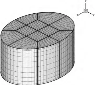
We use a spectral element method for the space discreti-zation of the equations in conservation form. The computa-tional domain is partitioned into Nenonoverlapping elements

⍀l 共1艋l艋Ne兲共Fig. 1兲. The reference coordinate system

xˆ⬅共xˆ,yˆ,zˆ兲 defines a cubic domain ⍀ˆ=关−1,1兴3_{. Data are}

ex-pressed as tensor products of Lagrange polynomials based on the Gauss-Lobatto-Legendre共GLL兲 quadrature points. Func-tions in the system coordinates x⬅共x,y,z兲 are of the form

u关xl共xˆ兲兴 =

兺

i=0 n_x

兺

_j=0ny

兺

_k=0nz u_ijkl h_inx共xˆ兲h j n_y_共yˆ兲h k n_z_共zˆ兲, _共5兲

where u_ijkl are the nodal basis coefficients, h_inx共xˆ兲 关respec-tively, h_jny共yˆ兲 and h

k

nz共zˆ兲兴 are Lagrange polynomials of degree

n_x 共respectively, n_y and n_z兲 based on the GLL quadrature points, and xl_共xˆ兲=(xl_共xˆ兲,yl_共xˆ兲,zl_{共xˆ兲) is the coordinate}

map-ping from the reference domain⍀ˆ to ⍀l.

In the projection scheme used for the momentum equa-tion, the linear terms are integrated implicitly and the non-linear terms explicitly. The first-order version of the scheme reads

⌬t−1_共u共n+1兲_{− u}共n兲_{兲 = − Ma共u}共n兲_·_ⵜ兲u共n兲₋_ⵜp共n+1兲

+ⵜ2u共n+1兲, 共6兲 where u共n兲refers to the velocity field at time tn⬅n⌬t. Each

time step is subdivided into three substeps. After the compu-tation of the nonlinear terms 共the first substep兲, a Poisson problem is formulated for the pressure using the boundary conditions proposed in Ref.12. This Poisson problem 共sec-ond substep兲 as well as the Helmholtz problems for the ve-locity components that constitute the final implicit substep of the scheme are solved using a variational formulation. Since a similar treatment is done for the heat equation, each time step involves the inversion of four Helmholtz problems共one for the temperature T and one for each velocity component兲 and one Poisson problem 共for the pressure兲. The inversions are performed using a Schur method taking full advantage of the tensorization in the z direction. Throughout the paper, we use Ne= 12 spectral elements.

To check the accuracy of the method, we compare our results with Refs.15and16. A direct comparison is difficult as the results of Refs.15and16are presented graphically. To check the accuracy of the critical Marangoni number, i.e., the

FIG. 1. View of the grid in an elliptical geometry. The grid has Ne= 12 macro-elements. Spatial resolution in each element is nx= ny= nz= 10, where

nx, ny, and nzare, respectively, the polynomial degrees of the interpolant in the x, y, and z directions.

(5)

primary bifurcation point for different aspect ratios, we have therefore employed three methods. The first uses Arnoldi’s method13 to calculate the largest eigenvalues of large linear systems. For the linear stability problem of the conduction state, this method yields the largest eigenvalues at discrete values of Ma. The critical Marangoni number corresponds to a zero maximum eigenvalue. In an A = 1 container with

nx⫻ny⫻nz= 10⫻10⫻10 interpolation yields Mac= 109.035.

The second method solves the system DF共Ma兲h=0, where DF denotes the linearized version of the discretized equations around the conduction state, and h

⬅共uijk l

,vijk l

, w_ijkl , T_ijkl 兲, 0艋i艋nx, 0艋 j艋ny, 0艋k艋nz, 1艋l

艋Ne, are the values of the three velocity components and

temperature at the grid points. This is a nonlinear system as both h and Ma are unknowns. This problem is solved using a Newton method as described in Ref.14. Consequently, no eigenvalue computation is involved. The method converges well as the number of grid points 共Fig. 2 and Table I兲 is

increased. The third method uses an extrapolation of fully nonlinear solutions to zero amplitude共Fig.3兲. For A=1 with

nx⫻ny⫻nz= 10⫻10⫻10, the extrapolation yields Mac

= 109.029. Thus all three methods are in excellent agreement with each other and with the values obtained in the previ-ously cited papers.

Our numerical method keeps track of the unstable eigen-values along each solution branch. For bifurcations that break the circular symmetry of the container, these

eigenval-ues are doubled. Thus it is important to characterize all so-lutions by their symmetry; this symmetry typically reflects the symmetry of the unstable eigenfunction responsible for the instability, although, as we shall see, this is not always the case.

In the following section, we will see how the multiplicity of the eigenvalues is reduced as the cylinder cross section becomes elliptical. We compute numerically the bifurcation diagrams for both O共2兲-symmetric 共circular兲 and

D2-symmetric 共elliptical兲 cross sections with our

continua-tion method. All primary bifurcacontinua-tions are steady-state bifur-cations since the eigenvalues of the linear stability problem are necessarily real.11,17Periodically we calculate the leading eigenvalues of the linearized system 共around the nonlinear state兲 using an adaptation of Arnoldi’s method described in Ref.13. When the number of positive eigenvalues changes, indicating a bifurcation, the method determines the param-eter interval in which the bifurcation occurs together with the associated eigenvector. The latter is used to initiate branch switching. Secondary bifurcation points are located from the intersection of pairs of nonlinear branches with different numbers of unstable eigenvalues, and for the aspect ratios used the results using a 10⫻10⫻10 grid agree well with the results of direct numerical integration. All calculations use Pr= 1 since the value of Pr has no effect on the primary bifurcations.

III. RESULTS

In this section, we describe the results for containers of both circular and elliptical cross section and different aspect ratios. The results are presented in the form of bifurcation diagrams, and use solid circles to indicate primary

bifurca-FIG. 2. Evolution of the critical Marangoni number for the m = 1 mode with the grid spacing nx= nywhen Pr= 1, A = 1.5, and nz= 10共cf. Fig.11兲.

TABLE I. Critical Marangoni number Macfor different grids and aspect ratios.

nx⫻ny⫻nz 6⫻6⫻10 10⫻10⫻10 14⫻14⫻10 10⫻10⫻14

m = 1, A = 1 109.0726 109.0286 109.0283 108.9071

m = 0, A = 2.1 84.1408 84.0812 84.0810 84.0818

m = 1, A = 2.8 82.9163 82.7896 82.7832 82.7871

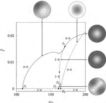
FIG. 3. Bifurcation diagram showing the maximum of the vertical velocity

wmas a function of the Marangoni number Ma. Snapshots show isovalues of the vertical velocity in the midplane of the cylinder. The orientation of the

m⫽0 states is nominally arbitrary. Parameters are⑀= 1, A = 1, and Pr= 1. Resolution is Ne= 12, nx= ny= nz= 10.

(6)

tions and secondary pitchfork bifurcations, while solid squares indicate saddle-node bifurcations, open circles indi-cate共secondary兲 Hopf bifurcations, and open triangles indi-cate collisions of a pair of complex eigenvalues on the posi-tive real axis; the latter, of course, does not correspond to a bifurcation. Primary bifurcations are labeled using the nota-tion Pm, Tm to indicate pitchfork 共P兲 and transcritical 共T兲

bifurcations to modes with azimuthal wavenumber m. In the following, we refer to eigenvalues with a negative共positive兲 real part as stable 共unstable兲 eigenvalues. Stability of each branch is indicated using the notation n − p, where n is the number of unstable real eigenvalues and p is the number of

pairs of unstable complex eigenvalues. Thus the number of

unstable eigenvalues is n + 2p. In the figures, we use solid

共dashed兲 lines to indicate linearly stable 共unstable兲 solutions.

We do not follow branches of time-periodic states. In many of the bifurcation diagrams, we include snapshots of the flow showing the vertical velocity w at midheight, with dark

共light兲 shading indicating w⬍0 共w⬎0兲.

Throughout the description that follows, we refer to states that are reflection-symmetric about x = 0 共y=0兲 as ␬y-symmetric共␬x-symmetric兲.

A. Aspect ratio A = 1

We begin with aspect ratio A = 1 and describe the changes that occur in the solutions of the nonlinear problem as the ellipticity⑀is reduced from⑀= 1. The diameter in the

x direction is kept equal to 1 throughout. We refer to Ref.18

for a similar study of square and nearly square containers. Figure3 shows the bifurcation diagram for the circular con-tainer. The figure displays the evolution with the Marangoni number of the maximum wm of the absolute value of the

vertical component of the velocity at the Gauss-Lobatto-Legendre nodes.19The value wm= 0 corresponds to the

con-duction state. Branches with wm⫽0 are characterized by the

azimuthal wavenumber m of the state, indicated in the label of the corresponding primary bifurcation.

Figure3 shows that the conduction state is stable up to Ma_P

1= 109.03. At this value of the Marangoni number the

conduction state undergoes a symmetry-breaking bifurcation that produces a branch of states with azimuthal wavenumber

m = 1. As a result, the eigenvalue that passes through zero at

MaP₁ is doubled, and the resulting bifurcation is a pitchfork

of revolution. The figure reveals that this bifurcation is su-percritical, and the resulting solutions are therefore stable

共modulo a zero eigenvalue associated with spatial rotations

of the pattern兲. We note, however, that the solutions are not invariant under a change in sign of wm. This is a consequence

of the different boundary conditions applied at the top and bottom of the container.

The second primary bifurcation occurs at MaP₂= 161.1

and is also a supercritical pitchfork of revolution, this time producing a branch of m = 2 solutions 共Fig. 4兲. These

solutions inherit the instability of the conduction state in MaP₁⬍Ma⬍MaP₂ and hence are doubly unstable.

More-over, like the m = 1 solutions, the m = 2 solutions are not in-variant under change of sign.

The final primary bifurcation we discuss occurs at

MaT₀= 164.2, and corresponds to a transcritical bifurcation to

an m = 0 state, i.e., to an axisymmetric state. Since this bifur-cation is unaffected by the O共2兲 symmetry of the system, only one eigenvalue passes through zero at Ma_T

0, with the

supercritical branch inheriting the four unstable eigenvalues of the conduction state, while the subcritical part is five times unstable.

Figure3 shows how these branches interact in the non-linear regime. The m = 1 branch terminates on the m = 0 branch above a saddle-node bifurcation 共Ma=162.34, indi-cated by a solid square兲 at a point labeled S1characterized by

a double zero eigenvalue. The bifurcation at S1is

mathemati-cally identical to that at P1: the m = 0 state loses stability with

decreasing Ma at a pitchfork of revolution at S1, and is

there-fore doubly unstable below S1 共and above the saddle node兲.

The prominent kink in the m = 1 branch just prior to S1 is a

consequence of increasing importance of the m = 0 contribu-tion, which shifts the local maximum in w to a new locacontribu-tion, and is not the result of a bifurcation. The figure shows that the m = 2 branch also terminates on the m = 0 branch, but this time below the saddle node, at a point labeled S2. Once

again, at this point there is a double zero eigenvalue. We find that above S2共and below the saddle node兲 the m=0 branch is

three times unstable; it follows that the m = 2 branch near S2

must be four times unstable, and hence that the m = 2 branch must undergo a Hopf bifurcation between P₂and S₂, a con-clusion that has been verified numerically 共Fig.4兲. Indeed,

the complex unstable eigenvalues created at the Hopf bifur-cation collide on the positive real axis with increasing Ma, before one of them reaches zero at S₂; the other zero eigen-value at S2 comes from rotations of the m = 2 states. The

number of unstable eigenvalues along each solution branch is indicated in the figure, and is consistent with the above theoretical expectation. Since the Hopf bifurcation preserves the symmetry of the m = 2 state, the resulting共unstable兲 os-cillations are standing waves, and likely disappear in a global bifurcation involving the m = 0 state.

(7)

It will have been noticed that the m = 1 and m = 2 states are both oriented at 45° to the x axis. This is a consequence of the structure of the numerical grid used to compute the solutions共Fig.1兲. The grid used is not rotationally invariant

but has in fact residual D4 symmetry. This symmetry group,

the symmetry of a square, is generated by two reflections,␬x

in the x axis and⌸xyin the line x = y. As discussed below, the

small perturbations due to the structure of the grid split each of the m = 1 and m = 2 branches into a pair of branches, one consisting of states with ␬x symmetry and the other of

⌸-symmetric states; each branch is produced in a standard

pitchfork bifurcation that come in in close succession. It turns out that in each case the grid selects the⌸-symmetric state as the first state that sets in. A similar observation ap-plies to the termination point S2, which is also split by the

grid. Both m = 2 branches undergo the Hopf bifurcation to standing oscillations prior to their termination on the m = 0 branch.

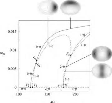
We now turn to a discussion of the corresponding results for a slightly elliptical container, characterized by⑀= 0.98. Although the resulting ellipticity is small, this value is still sufficiently far from⑀= 1 that the ellipticity effects ought to dominate the symmetry-breaking effects due to the grid. It should be mentioned that the elliptical deformation of the container cross section changes the symmetry of the problem to D2, the symmetry group of a rectangle, a smaller

symme-try group than D4. The former is generated by the two

reflec-tions␬xand␬y, and in contrast to␬xand⌸ these commute.

Figure5shows that this change in the symmetry of the prob-lem results in a substantial change in the bifurcation dia-gram. Since the primary bifurcations can only lead to␬x- and

␬y-symmetric states, the multiple bifurcations at P1 and P2

are strongly affected. Figure5shows that P1is split, with the

␬y-symmetric states coming in first, followed by the

␬x-symmetric states; the former are stable, while the latter

are once unstable. The bifurcation at P2 is also split,

result-ing in a transcritical bifurcation to D2-symmetric states and a

pitchfork to ⌸-like states 关Fig. 6共b兲兴. In fact, these states,

which come in at the point labeled P₂

⬘

, have exact ⌸ sym-metry at zero amplitude, but with increasing amplitude their plane of symmetry rotates monotonically, reaching 45° by the time the branch terminates at S₂

⬘

. The reason for this unexpected behavior will be explained below. Figure 6共b兲

also shows that one of the transcritical branches created in the breakup of P2 connects to the large-amplitude

axisym-metric states at S₁

⬘

, while the other undergoes a saddle-node bifurcation before connecting to the second transcritical bi-furcation T0; the latter is merely the共slightly perturbed兲

tran-scritical bifurcation T0 present in the O共2兲-symmetric case;

the same notation is therefore used to refer to it. This con-nection contains a Hopf bifurcation to standing oscillations

wmas a function of the Marangoni number Ma. Snapshots show isovalues of the vertical velocity in the midplane of the cylinder. Parameters are

⑀= 0.98, A = 1, and Pr= 1. Resolution is Ne= 12, nx= ny= nz= 10.

(8)

with D2 symmetry, but the resulting oscillations are

neces-sarily unstable. It should be noted that this bifurcation is present after S₂

⬘

; for ⑀closer to ⑀= 1, the order of these bi-furcations is reversed, while a second Hopf bifurcation is present on the branch of⌸-like states connecting P₂

⬘

to S₂

⬘

. Finally, the forced symmetry breaking to D2 also splits the

termination point S1 共Fig. 3兲, with the result that the

␬y-symmetric states transfer stability to the D2-symmetric

states arising from the axisymmetric states 关at S1 in Fig.

6共a兲兴, while the unstable branch of␬x-symmetric states

ter-minates on the D2-symmetric states just below关at S1

⬘

in Fig.

6共a兲兴. Once again the number of unstable eigenvalues along

each branch is indicated in the figure.

Figure 7 shows the corresponding results for ⑀= 0.90, i.e., for larger ellipticity. The broad features of the bifurca-tion diagram are similar. The main difference involves the branch of D2-symmetric states connecting the two primary

transcritical bifurcations. Figure 7 shows that this branch now undergoes an additional saddle-node bifurcation on the right; the termination point S₂

⬘

of the⌸-like states falls on the part of the D₂branch just below this saddle node. Moreover, the secondary Hopf bifurcation is now absent; this bifurca-tion collides with the saddle-node bifurcabifurca-tion with increasing ellipticity, and disappears via the so-called Takens-Bogdanov bifurcation. This bifurcation is then followed by a second

共and different兲 codimension-2 bifurcation at which S2

⬘

passes

through the saddle node.

Figure 8 shows the corresponding results for ⑀= 0.75. For this value of⑀ the order of the primary bifurcations is reversed. The reason for this is indicated in Fig. 9, which shows the linear stability thresholds for m = 1 modes in the

共⑀, Ma兲 plane. The figure shows that outside the region 0.8⬍⑀艋1, the mode that first sets in is the mode with ␬x

symmetry; the first unstable mode is␬y-symmetric only in

the range 0.8⬍⑀艋1. Because of the mode exchange that

takes place near⑀= 0.8, the␬x-symmetric states must transfer

their stability to the␬y-symmetric states in the nonlinear

re-gime. Figure10 shows that this transfer of stability occurs via a stable branch of mixed states, i.e., a branch of states with no symmetry. As a result, the stable large-amplitude states, away from the primary bifurcation, continue to be the ␬y-symmetric states.

FIG. 9. Critical Marangoni number Macas a function of the ellipticity⑀. The azimuthal wavenumber is m = 1. Parameters are A = 1 and Pr= 1. The primary bifurcation with⑀= 1 is split into two successive bifurcations: solid line indicates␬x-symmetric states, dashed line␬y-symmetric states. Resolu-tion is Ne= 12, nx= ny= nz= 10.

(9)

B. Aspect ratio A = 1.5

Figure 11 shows the linear stability thresholds for

A = 1.5, again as a function of ⑀. The primary instability is always to m = 0-like states, followed for⑀⫽1 by a transition at larger Ma to a succession of m = 2 states. At yet larger values of Ma共not shown兲, one finds a pair of transitions to

m = 1 states as well.

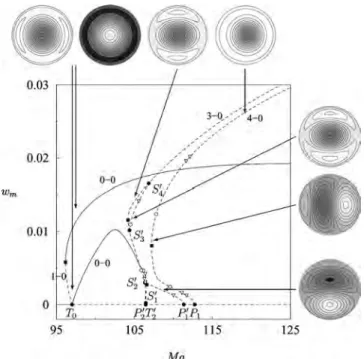
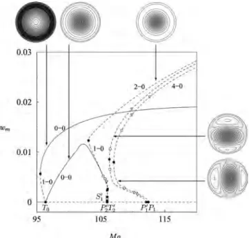
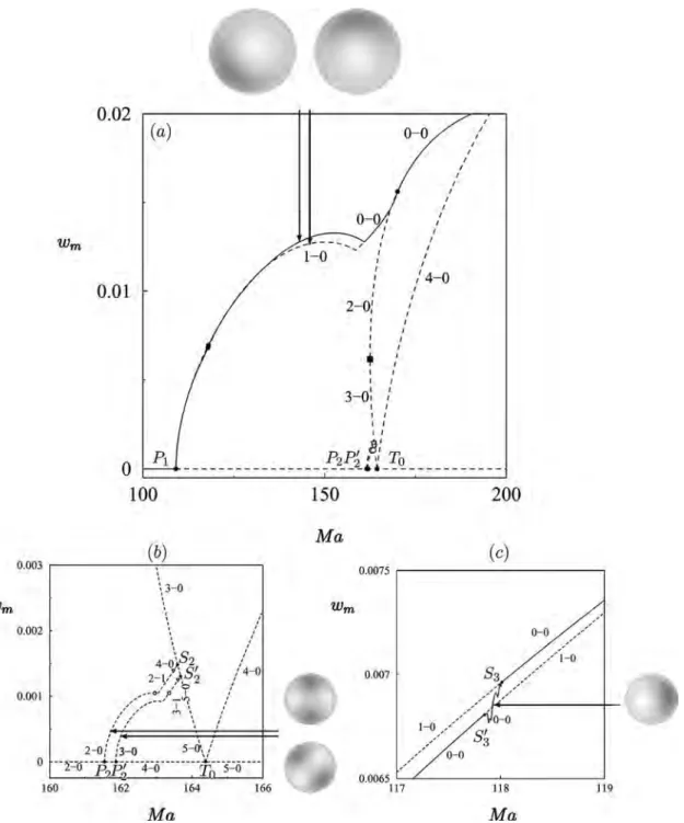
In the next set of figures, we examine the resulting be-havior in the nonlinear regime. Figure12shows the bifurca-tion diagram for ⑀= 1 with high resolution to minimize the effects of the computational grid. The primary bifurcation at T0 共MaT₀= 96.19兲 is transcritical and produces a stable

m = 0 branch of states with fluid descending in the center and

an unstable branch of states with ascending fluid in the cen-ter. The latter turns around at a saddle-node bifurcation 共in-dicated by a solid square兲 and acquires stability, remaining stable at larger values of Ma. In addition, a branch of m = 2 states bifurcates from the conduction state in a pitchfork of revolution at P₂共Ma_P

2= 105.87兲 and does so supercritically.

The resulting states are once unstable near onset, but become twice unstable above a saddle-node bifurcation共indicated by a solid square兲, before stabilizing via a 共subcritical兲 Hopf bifurcation. As a result, the m = 2 branch acquires stability before its termination on the共supercritical兲 m=0 branch at

S1. This bifurcation is again a pitchfork of revolution and

destabilizes the m = 0 states at larger values of Ma; for future reference, we emphasize that these states have a pair of un-stable eigenvalues and are hyperbolic, i.e., none of the eigen-values along this branch are close to zero and hence subject to qualitative change under small perturbation, such as the introduction of nonzero ellipticity. It follows that at large Ma, the only stable states are the axisymmetric states with ascending fluid in the center, as expected on physical grounds. Finally, at MaP₁= 112.35 the conduction state loses

stability to solutions with m = 1. The resulting pitchfork of revolution is subcritical, implying that the m = 1 states are initially four times unstable. Figure12shows, however, that despite the high resolution used, some effects of the compu-tational grid remain. These are most noticeable in the split-ting of the m = 1 branch emanasplit-ting from P1, and in the

pres-ence of the bifurcation points S3and S3

⬘

. These effects will be

discussed in greater detail in the following section.

Figure 13shows the corresponding bifurcation diagram for⑀= 0.98. We see a dramatic effect: the primary pitchforks of revolution are both split, P2into a pitchfork P2

⬘

to⌸-like

states and a transcritical bifurcation T₂

⬘

to ␬x-symmetric

FIG. 10. Closer view of Fig.8showing exchange of stability between␬x -and␬y-symmetric states via a stable branch of nonsymmetric states.

FIG. 11. Critical Marangoni number Macas a function of the ellipticity⑀. The continuous line refers to Mac共T0兲, the dashed line to Mac共P2⬘兲, and the

dot-dashed line to Mac共T2⬘兲. Parameters are A=1.5 and Pr=1. Resolution is Ne= 12, nx= ny= nz= 10.

wmas a function of the Marangoni number Ma. Snapshots show isovalues of the vertical velocity in the midplane of the cylinder. The orientation of the

m⫽0 states is nominally arbitrary. Parameters are⑀= 1, A = 1.5, and Pr= 1. Resolution is Ne= 12, nx= ny= nz= 10.

(10)

states 关Fig. 14共a兲兴, and P1 into a pair of pitchfork

bifurca-tions producing ␬y-symmetric states 共P1

⬘

兲 and␬x-symmetric

states 共P1兲, respectively 关Fig. 14共d兲兴. At the same time, the

primary bifurcation 共labeled T0兲 remains transcritical,

al-though the states that are produced are now D2-symmetric

and not axisymmetric. In addition, the secondary bifurcation at S1 is “unfolded” with the result that the supercritical

branch originating at T0 now connects to the supercritical

branch emanating from T₂

⬘

, while the subcritical branch at T₂

⬘

connects to the large-amplitude unstable m = 0-like state.

As in the A = 1 case, the unstable ⌸-like states rotate through 45°关Fig.14共a兲兴 along the branch before the branch

terminates on the doubly unstable supercritical part of the transcritical branch at a point labeled S₁

⬘

, below a saddle-node bifurcation at which the branch turns around toward smaller values of Ma 关Fig. 14共c兲兴. At the termination, the

number of unstable eigenvalues on the transcritical branch decreases to one, but at the saddle node it increases back to two, before a Hopf bifurcation stabilizes the branch. Alterna-tively, viewed from the perspective of the supercritical branch produced at T0, the solutions with descending fluid in

the center lose stability with increasing Ma at a Hopf bifur-cation关Fig.14共c兲兴. However, no stable oscillations have been

found in the vicinity of this bifurcation, suggesting that this bifurcation remains subcritical. In contrast, the subcritical part of the transcritical branch T₂

⬘

remains unstable through-out, and is three times unstable at large values of Ma关Fig.

14共b兲兴. The branch of␬y-symmetric states emerging from P1

⬘

now terminates at S₂

⬘

on the subcritical branch created at T₂

⬘

. In addition, there is a second segment of␬y-symmetric states

that extends from S₃

⬘

to S₄

⬘

and brackets the saddle node on the branch of subcritical D2-symmetric states emerging from

T₂

⬘

. In contrast, the branch of ␬x-symmetric states emerging

from P₁turns around at a saddle node and extends to larger values of Ma, where it is ultimately four times unstable关Fig.

14共d兲兴. A pair of Hopf bifurcations brackets the saddle node

but the associated oscillations are necessarily unstable. De-spite this, stable periodic oscillations are found near the saddle node in the interval 107.24⬍Ma⬍107.26, between the saddle-node bifurcation and the Hopf bifurcations. These oscillations grow in amplitude with increasing Ma共Fig.15兲

and are␬_x-symmetric共Fig.16兲, i.e., they share the symmetry

of the steady states on the branch emanating from P1, but

their relation to this branch remains unclear.

The bifurcation diagram shown in Fig.13possesses two unexpected features. First, the stability assignments indicate that the two large-amplitude branches have three and four unstable eigenvalues, respectively. In contrast, the m = 0 branch in Fig.12is only twice unstable, and for small per-turbations of the domain this stability assignment should be inherited by the corresponding D2 branch in Fig.13. In

ad-dition, we expect the presence of a third branch at large Ma, since the deformation of the domain is expected to split the

m = 1 branch into two distinct branches. To reconcile Fig.13

with Fig.12, we have therefore recomputed the bifurcation diagram for⑀= 0.995共Fig.17兲. The figure confirms that our

expectation is correct, and indicates that⑀= 0.98 is in fact a

large perturbation. Indeed, as ⑀ decreases, the branch of ␬y-symmetric states collides with the branch of

D2-symmetric states, and breaks into two segments. The first

of these terminates at S₂

⬘

关Fig. 14共c兲兴 while the second

ex-tends between S₃

⬘

and S₄

⬘

关Fig. 14共b兲兴. Evidently, as ⑀ de-creases, the bifurcation point S₄

⬘

moves in from large ampli-tudes and is responsible for the unexpected stability properties of the D₂-symmetric states at these amplitudes, as well as for the absence of the third large-amplitude branch. Finally, Fig. 17also reveals the presence of a pair of Hopf bifurcations on each of the branches bifurcating from P1and

P₁

⬘

, each of which brackets a saddle node. The presence of these bifurcations provides strong evidence for the presence of the corresponding bifurcations in the⑀= 1 case in the in-finite resolution limit. In addition, the Hopf bifurcations on both of the branches bifurcating from T₂

⬘

converge to the corresponding Hopf bifurcation in the⑀= 1 case共Fig.12兲.

C. Effects of the numerical grid

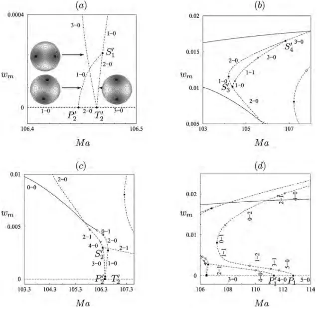
In this section, we examine the effects of the numerical grid noticed already in Fig.12. For this purpose, we decrease the resolution to nx= ny= 6. Figure18for A = 1 shows that the

grid splits the primary bifurcation P2to m = 2 states into two

successive bifurcations even when⑀= 1. Associated with this splitting is the splitting of the termination point S2;

more-over, both branches inherit the Hopf bifurcation present in Fig.3. In contrast, the primary bifurcation P1 is not split by

the grid, although the branches that emanate from it are. This branch splitting is responsible for the transfer of stability at finite amplitude between these two branches; this transfer occurs via a secondary branch of mixed states 关Fig.18共c兲兴

and is a consequence of the fact that the m = 1 states have a zero eigenvalue, associated with rotations, when⑀= 1. Figure

19 shows the corresponding results using the total kinetic

(11)

energyE as a measure of the solution amplitude. This proce-dure confirms that the splitting is due to the symmetry of the grid, and not an artefact produced by changes in the location of the maximum of兩w兩 with respect to a collocation point.

Figure 20 shows a blowup of some of the branches in Fig. 12, and demonstrates the effect of the computational grid even with the 10⫻10⫻10 resolution. The figure shows that the pitchfork at P₂ is split by the grid into two nearby

共pitchfork兲 bifurcations 共P2, P2

⬘

兲, one of which is to states

with␬_xsymmetry and the other is to states with⌸ symmetry. Both branches that result undergo the same sequence of bi-furcations, and these converge on the corresponding bifurca-tions in the nominally infinite resolution limit. In contrast, the bifurcation P₁is not split, although two distinct solution branches emerge from it at finite amplitude. Moreover, Figs.

20共a兲and20共b兲 reveal the presence of one secondary Hopf bifurcation 共open circle兲 on each branch, but this time at quite different locations. Thus the grid has a different effect on different bifurcations. As a result, the stability assign-ments along the split branches depend on which branch is

considered, and care must be taken when using these types of numerical results to establish stability properties in the nomi-nally infinite resolution limit.

The effect is magnified at lower resolution, as revealed in Figs.21–23. Note in particular the proliferation of second-ary Hopf bifurcations 共open circles兲 on the m=1 branches

关Figs.22共b兲and22共c兲兴. In contrast, the saddle-node

bifurca-tions共solid squares兲 and the secondary bifurcations S₃and S₃

⬘

at which the branches exchange stability关Fig.22共d兲兴 remain

almost unchanged. The new Hopf bifurcations are respon-sible for the presence of a narrow interval of stability above the leftmost saddle node关Fig.22共d兲兴. Evidently, this interval

of stability is an artefact of the low resolution, and only the bifurcations that also appear in Fig.20are “real.” In contrast, the bifurcations along the m = 2 branches emanating from P2

and P₂

⬘

continue to track each other well共Fig.23兲, although

we can now discern the presence of a pair of secondary bifurcations S2and S2

⬘

at which these branches trade stability

prior to their termination at S1 and S1

⬘

, respectively

关Fig.23共b兲兴.

(12)

Figure 22 demonstrates that because of the grid, the

m = 1 branch is already split into a pair of hyperbolic

branches, and one expects, therefore, to find three branches at large amplitude, at least for sufficiently small ellipticity; for larger⑀, the first of the m = 1 branches collides with and eliminates the large-amplitude m = 0 branch, resulting in the presence at large amplitude of only two branches, one with three unstable eigenvalues and the other with four.

Once ⑀⫽1, it is the ellipticity that splits the various branches, and the grid structure plays only a minor, quanti-tative role. In the following section, we provide a theoretical explanation of these results.

IV. THEORETICAL DESCRIPTION

Simulations in an A = 1 circular cylinder reveal succes-sive bifurcations to m = 1, 2, and 0 states; at the m = 1, m = 2 bifurcations, two eigenvalues become positive simulta-neously, while at m = 0 only a single eigenvalue changes sign. The simulations also reveal that in the nonlinear regime the

m = 0 and m = 2 states interact. These states interact in the A = 1.5 case as well. To describe this 共codimension-2兲

inter-action, we write

w共r,␪,z兲 = Re兵a共t兲f共r,z兲exp 2i␪其 + b共t兲g共r,z兲 + ¯ , 共7兲 where w is the vertical velocity at the point共r,␪, z兲, and we suppose that both modes set in in close succession, so that any interaction occurs already at small amplitude. In a cylin-drical container, the equations for the amplitudes a 共com-plex兲 and b 共real兲 must commute with the following representation20,21 of the symmetry group O共2兲 of rotations and reflections of a circle:

共a,b兲 → 共ae2i␾_,b_{兲, 共a,b兲 → 共a¯,b兲,} _共8兲

corresponding to rotations through an arbitrary angle␾and reflection in the x axis. Thus

a˙ =␮a −兩a兩2a +␣1ab +␣2ab2+ ¯ , 共9兲

b˙ =␯b +␤兩a兩2₊_␥_b2₊ _{¯ ,} _共10兲

where␮and␯are bifurcation parameters, and␣1,␣2,␤, and

␥are real coefficients, cf. Ref.11. In writing these equations, we have chosen the cubic term to be stabilizing. There are two types of solutions:

共a,b兲=共0,b兲, corresponding to axisymmetric states;

these bifurcate transcritically at␯= 0.

共a,b兲, ab⫽0, corresponding to m=2 modes; these

bifur-cate in a pitchfork of revolution at␮= 0, and are accompa-nied by a nonzero value of b, i.e., these solutions are not symmetric with respect to w→−w, as observed in the simu-lations. As already mentioned, this is a consequence of the different boundary conditions at the top and bottom.

FIG. 15. Oscillations in the maximum vertical velocity wmas a function of time obtained at Ma= 107.24共solid line兲, Ma=107.25 共dashed line兲, and Ma= 107.26共dot-dashed line兲. Parameters are⑀= 0.98, A = 1.5, and Pr= 1. Resolution is Ne= 12, nx= ny= nz= 10.

FIG. 16. Snapshots of the oscillation present at Ma= 107.25 at six instants within one period. The oscillation is periodic and␬x-symmetric. Parameters are⑀= 0.98, A = 1.5, and Pr= 1. Resolution is Ne= 12, nx= ny= nz= 10.

(13)

The m = 2 branch terminates on the branch of axisym-metric states when␮+␣1b +␣2b2= 0; this bifurcation is also

a pitchfork of revolution.

A similar set of equations can be written down for the

m = 1 states. These are also accompanied by a nonzero

con-tribution from the axisymmetric state.

A. Grid effect in a circular domain

We now explore the effect of the D4 symmetry of the

computational grid. We do so by adding to the above equa-tions small terms that preserve the symmetry of the system under reflection in both the x and y axes, as well as in the

diagonals, but break rotational invariance. To this end we look at the bifurcations to m = 2 and m = 1 separately.

When m = 2, the breaking of O共2兲 down to D4symmetry

leads to an equation of the form

a˙ =␮a −兩a兩2a +␣1ab +␣2ab2+ ¯ +⑀¯ ,a 共11兲

where⑀Ⰶ1 and is real. A small term proportional to b can be added to the b equation as well. It follows that the m = 2 mode now sets in at␮= ±⑀instead of␮= 0, in other words, that the primary bifurcation has been split into two succes-sive bifurcations. The solution that sets in at ␮= −⑀ corre-sponds to real a and hence to states of the form w

FIG. 18.共a兲 Bifurcation diagram showing the maximum of the vertical velocity wmas a function of the Marangoni number Ma. Snapshots show isovalues of the vertical velocity in the midplane of the cylinder.共b兲,共c兲 Closer view of 共a兲. Parameters are⑀= 1, A = 1, and Pr= 1. Resolution is Ne= 12, nx= ny= 6, and

(14)

= a cos 2␪f共r,z兲+¯ which are invariant with respect to

re-flections in the x and y axes. In contrast, the solution that sets in at ␮=⑀ corresponds to purely imaginary a and hence to states of the form w =兩a兩f共r,z兲sin 2␪+_{¯ that are invariant} under reflections in the diagonals. We identify the former with the ␬x-symmetric states, and the latter with the

⌸-symmetric states.

In contrast, when m = 1, the requirement that rotation by 90° leaves the system invariant共i.e., a→ia兲 shows that the only linear term in a that can be added to Eq.共9兲is propor-tional to a itself. Consequently, the grid does not split the bifurcation to m = 1 states, although it may shift its location. At finite amplitude we have

a˙ =␮a −兩a兩2a +␣1ab +␣2ab2+ ¯ +⑀¯a3, 共12兲

where⑀is again real. Writing a =␳exp i␺leads to the con-clusion that␺= 0 or ␺=␲/ 4, indicating the presence of two distinct branches at finite amplitude given by ␳2₌_␮_˜_共1±_⑀_兲,

where ␮˜⬅␮+␣1b +␣2b2 and the ⫾ signs correspond to

␺= 0 and ␺=␲/ 4, respectively. The former are reflection-symmetric with respect to ␬x, the latter with respect to ⌸.

Moreover, the ␺= 0 共␺=␲/ 4兲 is stable 共unstable兲 when ⑀⬎0 and vice versa. These stability assignments are

modi-fied in the obvious fashion when the bifurcation is subcritical or there are additional unstable eigenvalues that are inherited from the a = 0 state.

B. Elliptical domain

We suppose that the cylinder is distorted into an ellipse, and that this distortion is small. This distortion preserves the conduction state a = b = 0 but breaks the O共2兲 symmetry down to D2, the symmetry of a rectangle. The symmetry is

generated by reflections in the x and y axes. In addition, we include the symmetry breaking due to the grid. As already mentioned, the grid has symmetry D4 and thus breaks the

rotational symmetry of the system in a different way. In the following, it is important that the symmetries of the ellipse

are also symmetries of the grid. To incorporate both of these symmetry-breaking effects, we add to Eqs.共9兲 and共10兲 the largest terms that break the O共2兲 symmetry in the required fashion, while preserving invariance under reflection in the x and y axes. The results depend on the azimuthal wavenumber

m.

We begin with the interaction between the m = 1 and

m = 0 modes. In this case, the symmetry x→−x acts by

共a,b兲→共−a¯,b兲, while y→−y acts by 共a,b兲→共a¯,b兲. It

fol-lows that

a˙ =␮a −兩a兩2a +␣1ab +␣2ab2+ ¯ +⑀¯a3+␦¯ ,a 共13兲

b˙ =␯b +␤兩a兩2+␥b2+ _{¯ ,} 共14兲 where␦Ⰶ1 measures the ellipticity of the container, and is real. The resulting linearized equations are uncoupled: ␬x-symmetric states bifurcate from 共0, 0兲 at ␮= −␦, while

␬y-symmetric states come in at ␮=␦. Weakly nonlinear

analysis near each of these bifurcation points shows that these bifurcations are pitchforks. The analysis confirms the results of numerical continuation in the vicinity of the bifur-cation to the m = 1 state in both A = 1 and 1.5 cylinders 共com-pare Fig.3 with Fig.5, and Fig.12with Fig. 13兲.

We next turn to the interaction of the m = 2 and m = 0 modes. This time both x→−x and y→−y act by 共a,b兲

→共a¯,b兲, and we obtain

a˙ =␮a −兩a兩2a +␣1ab +␣2ab2+ ¯ + 共⑀+␦0兲a¯ +␦1b,

共15兲

b˙ =␯b +␤兩a兩2+␥b2+ _{¯ +}1₂␦₂共a + a¯兲. 共16兲 In these equations,⑀Ⰶ1 continues to represent the effect of the grid while the␦jⰆ1 break the remaining D4 symmetry

further, down to D2. Note that the symmetry requirement

permits the inclusion of the term␦0¯ at linear order; thus ina

this case the grid effect can in effect be absorbed in the

FIG. 19. 共a兲 Bifurcation diagram showing the kinetic energy E⬅兰⍀共u2+v2_{+ w}2_{兲d⍀ as a function of the Marangoni number Ma. 共b兲 Closer view of 共a兲.}

(15)

coefficient␦0, although we do not choose to do so. It follows

that ⑀⫽0 provides the dominant symmetry breaking effect only in circular domains.

With a⬅␳exp i␺ and␧⬅⑀+␦0, we have

␮␳−␳3+␣1␳b +␣2␳b2+␧␳cos 2␺+␦1b cos␺= 0,

共17兲 ␧␳sin 2␺+␦1b sin␺= 0, 共18兲

␯b +␤␳2+␥b2+␦2␳cos␺= 0. 共19兲

It follows that there are two types of solutions, satisfying sin␺= 0 and 2␧␳cos␺+␦1b = 0, respectively. In the former

case, a is real and can take either sign:

␮a − a3+␣1ab +␣2ab2+␧a +␦1b = 0, 共20兲

␯b +␤a2₊_␥_b2₊␦

2a = 0. 共21兲

Reconstructing the solution共7兲, we find

w共r,␪,z兲 = af共r,z兲cos 2␪+ bg共r,z兲 + ¯ . 共22兲 This solution describes a solution with D2 symmetry,

i.e., with two orthogonal axes of reflection. Moreover, the sin␺= 0 state sets in at

␮= −␧ +␦1␦2

␯ , 共23兲

representing the threshold shift due to both the grid and the elliptical distortion. A weakly nonlinear calculation near this point shows that

␮= −␧ +␦1␦2 ␯ +

冋

␣1␦2 ␯ + ␤␦1 ␯ + ␦1␦2 2_␥ ␯3

册

␳+ ¯ , 共24兲

indicating that this bifurcation becomes transcritical once the circular domain is distorted共␦1⫽0 and/or ␦2⫽0兲.

We examine next the bifurcation to the sin␺⫽0 branch. Since

FIG. 20. Closer view of Fig.12.共a兲 and 共b兲 show the two branches of m=1 states due to the grid, together with their stability assignments, while 共c兲 shows the transfer of stability between these branches.共d兲 shows the splitting of the m=2 branches emerging from P2, also due to the grid. In contrast to共a兲 and 共b兲,

(16)

cos␺= − ␦1b

2␧␳ 共25兲

the angle␺ will vary along the branch as a consequence of the variation of the amplitude ratio b /␳ with the bifurcation parameter␮. Equations共17兲and共19兲become

␮−␧ −␳2+␣1b +␣2b2= 0, 共26兲 ␯b +␤␳2+␥b2−␦1␦2b 2␧ = 0, 共27兲 implying that ␮=␧ +

冉

−␯−␤␣1+ ␦1␦2 2␧

冊

b ␤+ O共b2兲, 共28兲 ␳2₌

冉

₋_␯₊␦1␦2 2␧

冊

b ␤+ O共b2兲. 共29兲

The bifurcation at ␮=␧ is therefore a pitchfork: ␳⬃共␮−␧兲1/2_{. Equation} _共25兲_{now shows that cos}_␺ _vanishes

共␺→␲/ 2兲 as ␮→␧, while cos␺→1 共␺→0,␲兲 as ␮ in-creases. Consequently, the spatial phase␺/ 2 of the pattern gradually rotates with increasing supercriticality, and the to-tal amount of rotation from the primary bifurcation to the end of the branch is ±␲/ 4 as found in the numerical simu-lations. This rotation is evidently a consequence of the inter-action between the m = 2 and m = 0 modes, and is present whenever 共⑀+␦0兲␦1⫽0, however small, a situation that we

expect to be satisfied generically in elliptically distorted do-mains; the simulations show that the phase rotation persists even when the corresponding primary bifurcations are far apart, and the codimension-2 analysis just described no longer applies.

The bifurcation from the axisymmetric state to m = 2 at

S₁共Fig.12兲 is of the same type as P₁. As a result, the effect of the grid is described by

a˙ =␮a −兩a兩2a + _{¯ +}⑀¯ .a 共30兲

There are two types of solutions, with a real or pure imagi-nary; these set in at␮=⫿⑀, respectively, and correspond to states with␬xand⌸ symmetry, as observed in Fig.23.

Like-wise, in the absence of the grid, the effect of finite ellipticity is captured by the equation

a˙ =␮a −兩a兩2a + ¯ +␦0, 共31兲

where 0⬍兩␦₀兩Ⰶ1 is a real parameter.22Thus a must be real, and for fixed␦₀ the equilibria satisfy a cubic equation. One branch grows monotonically from negative to positive␮and is stable throughout; two other 共disconnected兲 solutions ap-pear via a saddle node and are present in␮⬎3共␦0/ 2兲2/3only.

Both are unstable. These predictions agree exactly with the results shown in Fig.17near S₁; evidently, the ellipticity in this figure overwhelms the effect of the grid responsible for the splitting of the m = 2 branches. It should be observed, however, that Eq.共31兲does not capture all aspects of the loss of symmetry;22 indeed, very close to S1 a more complete

“unfolding” is provided by

a˙ =␮a −兩a兩2a + _{¯ +}␦1¯ +a ␦0. 共32兲

This equation shows, by analogy with our discussion of the bifurcation at P1, that small intervals of secondary branches

with a rotating phase may also be present, and it is precisely these that are required to reconcile the splitting of the m = 2 branch when⑀= 1 into␬x- and⌸-symmetric branches 共Fig.

23兲 with the behavior shown in Fig.17 for 1 −⑀Ⰶ1, which shows that the solutions on either side of S1 connect to␬x

-and␬_y-symmetric branches.

Finally, near the primary bifurcation T₀ 共i.e., ␯= 0兲, we find that ␯= ␦1␦2 ␮+␧+

冋

−␥− ␦1␦2␣1 共␮+␧兲2− ␦1 2_␤ 共␮+␧兲2

册

b + ¯ , 共33兲 showing that the bifurcation to the analogue of the m = 0 state

remains transcritical. The above results are consistent with

those presented in Figs.5,13, and17.

V. DISCUSSION

In this paper, we have examined the effect of changing the container shape on pattern formation in Marangoni con-vection in small aspect ratio containers. The present study parallels an earlier investigation of the effects of changing the shape of the container from square to slightly rectangular.18In the present case, the change of shape of the container from circular to elliptical has a similar effect, in that the finite ellipticity of the container splits multiplicity-2 eigenvalues, resulting not only in the appearance of multiple hyperbolic branches, but also of a variety of secondary bifur-cations, including some responsible for “mode-jumping” at finite amplitude. Although none of the secondary Hopf bifur-cations we have identified appears to be supercritical, i.e., none produces stable small-amplitude oscillations, we have

wm as a function of the Marangoni number Ma. Parameters are ⑀= 1,

(17)

nonetheless located stable periodic oscillations near the saddle-node bifurcation on the m = 1 branch when A = 1.5. At present, the origin of these unexpected oscillations remains unclear. However, it appears that these oscillations are not introduced by the elliptical distortion of the domain, in con-trast to the共quasiperiodic兲 oscillations studied in Ref.23.

For our computations, we have employed a code that could simultaneously be used to compute solutions in both circular and elliptical domains, and that could capture tran-sitions that shift a pattern off-center even in a circular con-tainer. The numerical scheme employed is more accurate than finite-element techniques but employs a grid that pos-sesses the symmetry D4. We have found, perhaps

surpris-ingly, that the orientation of the pattern can be pinned to the grid, and that this pinning persists even as the resolution of the grid is substantially increased. We have shown that the presence of such pinning can be understood using appropri-ate ideas from bifurcation theory, and that these ideas could

be extended to incorporate the interaction between the grid and the ellipticity of the container. Although limited in scope, the theory was in all cases confirmed by our computations.

It is significant that for A = 1, the mode that first becomes unstable is nonaxisymmetric; with increasing Marangoni numbers, the amplitude of this mode grows until a nonhys-teretic transition to an axisymmetric state takes place. In ex-periments on the Rayleigh-Bénard-Marangoni problem, Koschmieder and Prahl2 found that for 0.87艋A艋2.15, the first state observed was always axisymmetric, an observation that may be reconciled with the theory by including both the presence of surface deformation that is present in the experi-ments and the nontrivial effect of a finite Rayleigh number, also neglected in the present paper. On the other hand, the prediction that for A = 1.5 the primary instability will be a transcritical bifurcation to an m = 0 mode is consistent not only with microgravity experiments7 but also with ground-based experiments2 and the共extrapolated兲 results of Dauby

FIG. 22.共a兲–共d兲 Closer view of Fig.21showing exchange of stability between the two branches emerging from P1. Parameters are⑀= 1, A = 1.5, and Pr

(18)

et al.24 that do include finite Rayleigh number effects. How-ever, with increasing aspect ratio, Dauby et al. predicted an onset of instability via an m = 1 mode, followed by m = 2 and more complex structures, while the m = 1 state is apparently absent from Koschmieder and Prahl’s experiments.

Our results suggest distinct protocols for carrying out more detailed experiments. In particular, when the primary instability is a transcritical bifurcation to an axisymmetric mode, it is vitally important to examine perturbations with both downflow and upflow in the center of the container. Specifically, our results for A = 1.5 show that the primary instability leads to a stable m = 0 state with downflow in the center, and that this state remains stable until a secondary bifurcation, where it acquires an m = 2 contribution; at larger Ma this mixed state loses stability to growing oscillations, and a hysteretic transition to a stable m = 0 state with upflow in the center takes place. This state remains stable for larger Ma. In fact, these upflow states are stable down to a saddle-node bifurcation where the system undergoes a hysteretic transition back to the conduction state. It is significant that upflow states of this type have indeed been observed under microgravity conditions.7When the domain is deformed into an ellipse, the downflow m = 0 and m = 2 branches form a single continuous branch, but the hysteretic transition to the upflow state with increasing Ma remains. An appropriate ex-perimental protocol focusing on downflow states near onset could in principle confirm the presence of both hysteresis loops and detect any共finite-amplitude兲 oscillations that may be associated with the loss of stability of the downflow state. The results described here are largely insensitive to the precise value of the Prandtl number. In particular, for Pr= 7,

A = 1, the global properties of the bifurcation diagrams

are not drastically affected. For example, when ⑀= 1, the Marangoni number of the secondary bifurcation S1共Fig.3兲 is

hardly affected. When ⑀= 0.98, the only noticeable change occurs along the supercritical part of the branch emerging from T₂

⬘

. Here two saddle nodes are present in succession, and the eigenvalues change from 2-0 to 3-0 and then back to 2-0, thereby recovering the stability properties indicated in

Figs.5and6prior to the connection with the branch emerg-ing from P₁

⬘

. An additional change occurs along the subcriti-cal part of the branch emerging from T₂

⬘

: the Hopf bifurcation is now absent and is replaced by two saddle-node bifurca-tions. We have been unable, however, to recover the oscilla-tions observed when Pr= 1 and A = 1.5共Fig.15兲. This comes

as no surprise since in problems of this type, a lower value of Pr favors the presence of oscillations.

It is noteworthy that we have seen no evidence of the dynamics expected to arise from the interaction of the m = 1 and m = 2 modes in circular containers.25,26 The most dra-matic feature of this interaction is the presence, in certain parameter regimes, of structurally stable heteroclinic cycles connecting the m = 2 state with its rotations by ␲/ 4. Such cycles have been observed in A = 2.5 containers by Johnson and Narayanan5 and reproduced within weakly nonlinear theory by Dauby et al.;24see also Ref.7. Presumably this is so because the aspect ratios we have used are too far from the required codimension-2 point for this interaction.

ACKNOWLEDGMENTS

This work was supported in part by a CNRS Projet In-ternational de Cooperation Scientifique共PICS 3471兲 and by the National Science Foundation under Grant No. DMS-0305968.

1

H. Bénard, “Les tourbillons cellulaires dans une nappe liquide,” Rev. Gen. Sci. Pures Appl. 11, 1261共1900兲.

2

E. L. Koschmieder and S. A. Prahl, “Surface-tension-driven Bénard con-vection in small containers,” J. Fluid Mech. 215, 571共1990兲.

3

T. Ondarçuhu, G. B. Mindlin, H. L. Mancini, and C. Pérez-García, “Dy-namical patterns in Bénard-Marangoni convection in a square container,” Phys. Rev. Lett. 70, 3892共1993兲.

4

T. Ondarçuhu, J. Millán-Rodríguez, H. L. Mancini, A. Garcimartín, and C. Pérez-García, “Bénard-Marangoni convective patterns in small cylindrical layers,” Phys. Rev. E 48, 1051共1993兲.

5

D. Johnson and R. Narayanan, “Experimental observation of dynamic FIG. 23.共a兲,共b兲 Closer view of Fig.21showing exchange of stability between the two branches emerging from P2and P2⬘. Parameters are⑀= 1, A = 1.5, and

(19)

mode switching in interfacial-tension-driven convection near a codimension-two point,” Phys. Rev. E 54, R3102共1996兲.

6

R. Pasquetti, P. Cerisier, and C. Le Niliot, “Laboratory and numerical investigations on Bénard-Marangoni convection in circular vessels,” Phys. Fluids 14, 277共2002兲.

7

D. Schwabe, “Marangoni instabilities in small circular containers under microgravity,” Exp. Fluids 40, 942共2006兲.

8

M. F. Schatz and G. P. Neitzel, “Experiments on thermocapillary instabili-ties,” Annu. Rev. Fluid Mech. 33, 93共2001兲.

9

B. Hof, P. G. J. Lucas, and T. Mullin, “Flow state multiplicity in convec-tion,” Phys. Fluids 11, 2815共1999兲.

10

W. Meevasana and G. Ahlers, “Rayleigh-Bénard convection in elliptic and stadium-shaped containers,” Phys. Rev. E 66, 046308共2002兲.

11

S. Rosenblat, S. H. Davis, and G. M. Homsy, “Nonlinear Marangoni con-vection in bounded layers. Part 1. Circular cylindrical containers,” J. Fluid Mech. 120, 91共1982兲.

12

G. Em. Karniadakis, M. Israeli, and S. A. Orszag, “High-order splitting method for the incompressible Navier-Stokes equations,” J. Comput. Phys.

97, 414共1991兲.

13

K. Mamun and L. Tuckerman, “Asymmetry and Hopf bifurcation in spherical Couette flow,” Phys. Fluids 7, 80共1995兲.

14

A. Bergeon, D. Henry, H. BenHadid, and L. S. Tuckerman, “Marangoni convection in binary mixtures with Soret effect,” J. Fluid Mech. 375, 143 共1998兲.

15

P. C. Dauby, G. Lebon, and E. Bouhy, “Linear Bénard-Marangoni insta-bility in rigid circular containers,” Phys. Rev. E 56, 520共1997兲.

16

H. Herrero and A. M. Mancho, “On pressure boundary conditions for

thermoconvective problems,” Int. J. Numer. Methods Fluids 39, 391 共2002兲.

17

A. Vidal and A. Acrivos, “Nature of the neutral state in surface-tension driven convection,” Phys. Fluids 9, 615共1966兲.

18

A. Bergeon, D. Henry, and E. Knobloch, “Three-dimensional Marangoni-Bénard flow in square and nearly square containers,” Phys. Fluids 13, 92 共2001兲.

19

C. Canuto, M. Hassani, A. Quarteroni, and T. A. Zang, Spectral Methods

in Fluid Mechanics共Springer-Verlag, New York, 1987兲. 20

J. D. Crawford and E. Knobloch, “Symmetry and symmetry-breaking bi-furcations in fluid dynamics,” Annu. Rev. Fluid Mech. 23, 341共1991兲.

21

M. Golubitsky, I. Stewart, and D. G. Schaeffer, Singularities and Groups

in Bifurcation Theory共Springer-Verlag, New York, 1988兲, Vol. 2. 22

M. Golubitsky and D. G. Schaeffer, “A discussion of symmetry and sym-metry breaking,” Proc. Symp. Pure Math. 40, 499共1983兲.

23

A. Bergeon and E. Knobloch, “Oscillatory Marangoni convection in bi-nary mixtures in square and nearly square containers,” Phys. Fluids 16, 360共2004兲.

24

P. C. Dauby, P. Colinet, and D. Johnson, “Theoretical analysis of a dy-namic thermoconvective pattern in a circular container,” Phys. Rev. E 61, 2663共2000兲.

25

D. Armbruster, J. Guckenheimer, and P. Holmes, “Heteroclinic cycles and modulated travelling waves in systems with O共2兲 symmetry,” Physica D

29, 257共1988兲.

26

I. Mercader, J. Prat, and E. Knobloch, “Robust heteroclinic cycles in two-dimensional Rayleigh-Bénard convection without Boussinesq symmetry,” Int. J. Bifurcation Chaos Appl. Sci. Eng. 12, 2501共2002兲.