On the Regression and Assimilation for Air Quality Mapping Using Dense Low-Cost WSN

HAL Id: hal-03084455

https://hal.archives-ouvertes.fr/hal-03084455

Submitted on 21 Dec 2020

HAL is a multi-disciplinary open access

archive for the deposit and dissemination of

sci-entific research documents, whether they are

pub-lished or not. The documents may come from

teaching and research institutions in France or

abroad, or from public or private research centers.

L’archive ouverte pluridisciplinaire HAL, est

destinée au dépôt et à la diffusion de documents

scientifiques de niveau recherche, publiés ou non,

émanant des établissements d’enseignement et de

recherche français ou étrangers, des laboratoires

publics ou privés.

On the Regression and Assimilation for Air Quality

Mapping Using Dense Low-Cost WSN

Mohamed Anis Fekih, Ichrak Mokhtari, Walid Bechkit, Yasmine Belbaki,

Hervé Rivano

To cite this version:

Mohamed Anis Fekih, Ichrak Mokhtari, Walid Bechkit, Yasmine Belbaki, Hervé Rivano. On the

Regression and Assimilation for Air Quality Mapping Using Dense Low-Cost WSN. AINA2020 - 34th

International Conference on Advanced Information Networking and Applications, Apr 2020, Caserte,

Italy. pp.566-578, �10.1007/978-3-030-44041-1_51�. �hal-03084455�

On the regression and assimilation for air quality mapping

using dense low-cost WSN

Mohamed Anis Fekih, Ichrak Mokhtari, Walid Bechkit, Yasmine Belbaki, and Hervé Rivano

Abstract The use of low-cost Wireless Sensor Networks (WSNs) for air quality monitoring has recently at-tracted a great deal of interest. Indeed, the cost-effectiveness of emerging sensors and their small size allow for dense deployments and hence improve the spatial granularity. However, these sensors offer a low accu-racy and their measurement errors may be significant due to the underlying sensing technologies. The main aim of this work is to reconsider and compare some regression approaches to assimilation ones while taking into account the intrinsic characteristics of dense deployment of low cost WSN for air quality monitoring (high density, numerical model errors and sensing errors). For that, we propose a general framework that allows the comparison of different strategies based on numerical simulations and an adequate estimation of the simulation error covariances as well as the sensing errors covariances. While considering the case of Lyon city and a widely used numerical model, we characterize the simulation errors, conduct extensive simulations and compare several regression and assimilation approaches. The results show that from a given sensing error threshold, regression methods present an optimal sensor density from which the mapping qual-ity decreases. Results also show that the Random Forest method is often the best regression approach but still less efficient than the BLUE assimilation approach when using adequate correction parameters.

Mohamed Anis Fekih

Univ Lyon, Inria, INSA Lyon, CITI, F-69621 Villeurbanne, France, e-mail: [email protected] Ichrak Mokhtari

Univ Lyon, Inria, INSA Lyon, CITI, F-69621 Villeurbanne, France

Laboratoire de Methodes de Conception de Systemes (LMCS), ESI, Algiers, Algeria e-mail: ichrak.mokhtari@ insa-lyon.fr

Walid Bechkit

Univ Lyon, Inria, INSA Lyon, CITI, F-69621 Villeurbanne, France, e-mail: [email protected] Yasmine Belbaki

Univ Lyon, Inria, INSA Lyon, CITI, F-69621 Villeurbanne, France

Laboratoire de Methodes de Conception de Systemes (LMCS), ESI, Algiers, Algeria e-mail: [email protected] Hervé Rivano

1 Introduction

Air pollution is one of the major concerns in many cities worldwide. Indeed, millions of people live in cities where pollutant concentrations exceed standard health limits many times each year which poses serious health concerns. According to the World Health Organization (WHO), seven million deaths were attributable to the indoor and outdoor air pollution in 2016 [1]. Indeed, long-term exposure to air pollution can cause cancer and damage to the immune, neurological, and respiratory systems. In extreme cases, it can even cause death. In order to reduce the impact of air pollution, an efficient monitoring system is needed where the main aim is to generate accurate pollution maps in real time. Traditional monitoring stations are equipped with multiple sensors measuring a number of pollutants, such as carbon monoxide (CO), nitrogen oxides (NOx), ozone (O3) and particulate matter (PM)[2]. These monitoring stations give accurate concentrations but they are too big and expensive to be deployed everywhere [3]. In addition to measurement-based traditional monitoring, air pollution maps can be also obtained using numerical simulations of physical models. These models simulate the air pollution dispersion based on the locations of pollution sources, emission rates and meteorological data to estimate the pollutant concentrations.

The limits of traditional monitoring stations in terms of cost, size, flexibility and spatial granularity led to the emergence of small and low-cost air quality sensors. The wireless connection these sensors, forming a low-cost Wireless Sensor Network (WSN), presents many advantages compared to traditional air pollu-tion monitoring solupollu-tions. Indeed, the cost-effectiveness allows for dense and large deployments and hence improves the spatial granularity [4, 5, 6]. Moreover, the size and cost considerations offer more deploy-ment flexibility. However, low cost WSN present some problems and challenges to be addressed. The most significant of these is the low accuracy of the sensing probes. For instance, most low-cost gas probes are electrochemical which means they are very sensitive to temperature and humidity depending on the elec-trolyte. Moreover, this kind of probes present cross-reactivity with similar molecule types [7]. Optical parti-cle counter probes usually used as low-cost PM sensors are also less accurate than ground stations. Indeed, the given particle counts is sensitive to many parameters such as particle shape, color, density, humidity and refractive index. In addition, the conversion from particle counts to PM mass is based on theoretical models [7]. Furthermore, the high density of these sensors pushes us to reconsider the deployment approaches [8, 9] as well as the collected data analysis for air quality mapping.

In this paper we tackle these challenges while comparing regression and assimilation approaches, taking into account numerical model errors and sensing errors. To the best our knowledge this is the first work to compare regression and assimilation methods for air quality mapping using dense low-cost WSN data. The main contributions of this work can be summarized as follows:

1. We derive a generic framework that allows us to compare different regression and assimilation ap-proaches.

2. We characterize the errors of the SIRANE numerical model [10, 11, 12] based on a realistic data set. 3. We conduct extensive simulations and compare four regression approaches and one assimilation method

taking into account multiple errors of both measurements and the numerical model.

4. We derive some guidelines and insights for the choice of adequate approach depending on different pa-rameters such as the deployment density, the simulation error, the sensing error, etc.

2 Related Works

Air quality monitoring has attracted great attention in recent years. In order to tackle the pollution problem, we first need to build fine grained estimation maps. These maps allow us to assess the exposure of the population to pollution, detect highly polluted areas and warn the population if the recommended thresholds are exceeded. Generally, two types of approaches are used for air pollution mapping: spatial interpolation and data assimilation.

Spatial interpolation methods have been largely used in the literature and several works applied Land-Use Regression (LUR) techniques. Kerckhoffs et al. [13] propose a multiple regression model that generates av-erage annual concentrations of Ozone (O3) at a fine spatial scale (50m × 50m). Ozone concentrations were

measured at 90 sites covering the whole Netherlands. All sites were measured simultaneously during four campaigns of two weeks each spread over the seasons. Several explanatory variables were used, character-ising mainly roads, buildings, traffic and population density. This model allowed to reach a determination coefficient of 0.77.

Hasenfratz et al.[5] used mobile sensor nodes to collect ultra fine particle (UFP) data. Sensors were installed on top of public transport vehicles in the city of Zurich. Based on the collected measurements and land-use data, a LUR model was developed to create pollution maps with a spatial resolution of 100m × 100m. Twelve explanatory variables representing the traffic, the population and the city’s characteristics were examined to build the air quality models for UFP. The accuracy of models across various time scales were compared. Results show that low temporal resolution mapping achieves good results while high temporal resolution estimation presents high errors. To increase the accuracy of these models, past measurements were used in the modeling process which permitted to reduce the root mean square error by 26%.

Marjovi et al. [14], proposed two approaches for estimating the pollution level of UFP at desired time-location pairs in Lausanne in Switzerland. The first is a log-linear regression built over a virtual dependency graph based on land-use data. The second is a deep learning framework which can capture automatically the relationships between data based on autoecoders. Different land use, meteorological and traffic data were used to build these models, among them altitude, scope, density of population, buildings, industries, etc. The two approaches were evaluated against three canonical modeling techniques namely Basic Log-Linear regression model (BLL), Network-based Log-Linear regression (NLL) and Basic Log-Linear regression with Land-Use (BLL-LU). The results demonstrated the superiority of the proposed approaches and specifically the deep learning model over the canonical techniques.

Adam-Poupart et al. developed in [15] three interpolation methods: i) a land-use mixed-effects regression, ii) a Bayesian maximum entropy using both O3 monitoring station data and the land-use-mixed outputs

(BME-LUR), and iii) a kriging model for estimating the daily daytime average ozone concentrations from routine monitors in Quebec (Canada). Results showed the superiority of the BME-LUR as the best predictor followed by the LUR method and the kriging.

Data assimilation aims to efficiently combine numerical models with observations. It has been initially developed and used for meteorology until the 90’s [16]. After that, it has been applied in many other fields such as atmospheric chemistry and agronomy. Today it is used in many applications like the optimization of observation network and the correction of several numerical models’ errors in different fields.

In the air quality field, several assimilation-based approaches were proposed in the literature. Tilloy et al. [17] used the Best Linear Unbiased Estimator (BLUE) method to combine NO2 ground observations

provided by 9 fixed monitoring stations across Clermont-Ferrand city in France and a simulation at urban scale. The simulation has been carried out over the city every three hours for the whole year 2008 using a model called ADMS Urban. BLUE was computed every three hours when new simulated concentrations

were available and results showed that data assimilation corrected the problem of under estimation of NO2

concentrations when using only the model.

Kumar et al. [18] used a bias-aware optimal interpolation combined with Hollingsworth–Lönnberg method to estimate error covariance matrices to perform corrections on hourly simulated O3and NO2

con-centrations. The simulation has been performed using the regional-scale air quality model AURORA over Belgium for a summer and a winter month (June and December respectively). The monitoring network was composed of 73 monitoring stations. Results showed that data assimilation improved the simulation results with a root mean square error that went down from 27.9 to 12.6 for O3and from 17.4 to 11 for NO2.

In another work [19], NO2observations from Ozone Monitoring Instruments (OMI) aboard NASA Aura

satellite during November-December were combined with results of an air quality Model to improve air quality forecasts resulting in a spatial resolution of around 40 km x 55 km. The simulations showed that the RMSE was reduced by 15%. However, the resolution offered by satellite data is very low and does not allow air quality characterisation at a human scale.

The majority of data assimilation solutions are based in their validation on reference stations whose data are accurate. However it is not feasible to equip a large area with high-accuracy sensors due to their cost and complexity. Therefore, our first objective in this work is to propose a framework that allows comparing assimilation approaches to regression ones when using low-cost sensors. Our framework is based on numer-ical models, the characterization of their errors and the characterization of sensing errors. Another objective is to use this framework to compare the performances of different solutions and to derive some guidelines and insights.

3 Brief Overview on Regression and Data Assimilation for spatial mapping

We present in the section a brief background of some regression and assimilation approaches that we com-pare later. The main used notations are presented in Table 1.

Table 1 Main notations used in this work Symbol Description

xt _{Ground truth vector of pollution concentrations}

xb Background vector (simulated values)

σb Simulation (numerical model) standard deviation error

ym _{The observational vector (represents pollution measurements)}

σm Sensing (measurement) standard deviation error

xa _{The analyzed vector (represents the best estimation given}

by a mapping approach)

R The observational error covariance matrix B The background error covariance matrix H The observation operator

3.1 Spatial interpolation

Spatial interpolation bring together a set of techniques that estimate the concentration values at a given point as a weighted average of the measurements at surrounding observation points [20]. Land-Use-Regression (LUR) assume that pollutant concentrations at a given location depend on the surrounding environment, land-use and traffic characteristics [21].

Linear regression seeks to establish a linear relationship between the studied variable called the dependent variable and the variables likely to explain the phenomenon called independent or explanatory variables. The resulting model is then used to predict the concentration of a pollutant in a given location where no sensor is deployed. The most used explanatory variables in the air quality field are: humidity, temperature, wind speed, population, traffic intensity and road length [20]. K nearest neighbors (KNN) regression uses ‘feature similarity’ to predict values of any data points where no sensor is deployed. Similarity between the point to be predicted and the observation points is defined according to a distance metric applied to independent variables. The k nearest neighbors are the k closest points to the predicted point based on the defined metric. The concentrations at these neighbors are then used to estimate the concentration at the predicted point. Today other recent machine learning techniques such as random forest and Xgboost have emerged as serious competitors to state-of-the-art methods. Random forest (RF) also called decision forest [22] performs, in its most classical form, parallel learning on multiple decision trees built randomly and driven on different subsets of data using a bagging approach [23]. The main idea behind this technique is that the aggregate of the results of multiple predictors gives a better prediction than the best individual predictor. Indeed this allows to average noisy and unbiased models and thus create a model with low variance. Extreme gradient boosting abbreviated as Xgboost is also an ensemble learning method that combines the outputs from individual trees to make a prediction exactly like random forest. Xgboost and RF differ in the way the trees are built and the order and the manner the results are combined. In Xgboost, trees are built one at time, where each new tree helps to correct errors made by the previously-trained tree.

3.2 Data assimilation

One of the best assimilation methods used for air quality mapping is the Best Linear Unbiased Estimator (BLUE) [17]. BLUE uses the errors of both the background and the observations to estimate the state vector as follows:

xa= xb+ K(ym− Hxb_{) (1)}

Where xais the analyzed vector, xbthe background vector (simulated values using numerical models in our case), K the Kalman gain, ymthe observations vector (measurements given by the deployed sensors in our case), H the observation operator which is a matrix where hi j= 1 if the sensor i is deployed at position

j and hi j= 0 otherwise. The equation 1 means that the analysed vector is a correction of the background

vector with K(ym- Hxb).

While minimizing the sum of the squares of the estimation errors, BLUE gives the optimal Kalman gain as follows :

Where B and R are the covariance matrices of the background estimate and the observations respectively.

4 Methods and models

We present in this section the general methodology that we propose to compare different mapping ap-proaches. We present then our work to characterize the simulation errors and to generate the ground truth and measurements data sets. We present at the end of the section, the developed regression mapping models.

4.1 General Methodology

In order to compare different regression and assimilation approaches, we propose first to generate a large number of ground truth data sets based on physical models (numerical simulations) and an adequate es-timation of the simulation error variance-covariance matrix. We explain in the following sub-sections the approach that we use in order to estimate the simulation error variance-covariances.

Once the ground truth data sets generated, we generate for each one a large number of observations (pollutant concentrations) in positions where low-cost sensors are deployed. This generation will take into account the ground truth realizations as well as the measurements’ errors variance-covariance matrix. Based on the measurement realizations, simulation values and ground truth realizations, different regression and assimilation methods can be developed and compared.

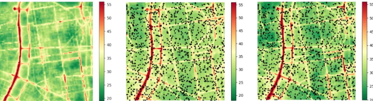
Fig. 1 NO2 concentrations of the area of interest (a) a realization of the ground truth; (b) Random forest regression based estimation; (c) BLUE assimilation based estimation

4.2 Area of interest and simulation data set

Without loss of generality, we consider in this work, simulations generated by the model SIRANE [10, 11, 12]. SIRANE is a stationary model designed for urban areas and is widely used by the certified associations of air quality monitoring in France. The used simulations give the Nitrogen-Dioxide concentrations in Lyon

city (France) in 2008. We consider in this work a 25km2_{area of interest with a spatial resolution of 20m x}

20m. This area corresponds to the center of Lyon and its immediate vicinity (see Figure 1 (a)).

4.3 Characterization of the variance of simulation errors

In order to characterize the variance of the simulation errors, we used NO2concentration values provided

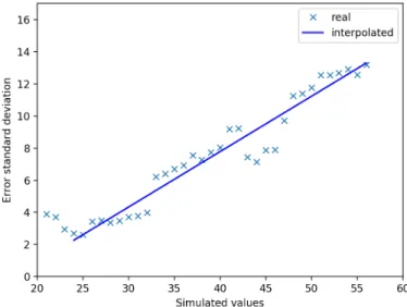
by 16 reference stations in Lyon and compared them to the simulated concentrations of SIRANE . We considered monthly values in both cases. For each simulated value z, we computed the standard deviation of the errors associated to simulated values in z ± 5ug/m3. Figure 2 shows that the model’s error standard deviation, σb, depends linearly on the pollutant concentration starting from a given threshold z0:

σb(z) = α(z − z0) + β , z ∈ [z0, +∞[ (3)

Were z is the simulated value. As shown in Figure 2, a linear regression with z0= 24 ug/m3results in

α = 0.344 and β = 2.27 ug/m3with a high R2value ( R2= 0.94).

Fig. 2 Error standard deviation Vs Simulation Values

4.4 Ground truth and measurements generation

Based on the variances of simulation errors and correlation coefficients wpq, we generate the

variance-covariance matrix. In this work, we consider the correlation coefficient as a function of the distance [9] given as: wpq= e−δ ˙dpq, were δ is the attenuation coefficient of the correlation function and dpqis the

distribution, we generate a large number of ground truth data sets based on the simulated values and the computed variance-covariance matrix.

Once the ground truth data sets generated, we generate for each ground truth set, a large number of observations (measurements) in positions where low-cost sensors are deployed. Sensors’ measurements on their side are generated using a normal distribution since the sensing errors are not correlated with each other. Hence, the measurement error variance-covariance matrix that we note R is given by: R = v0I, where

v0is the vector of measurements’ error variance and I is the identity matrix.

4.5 Dependant variables for regression methods

The performance of regression methods rely mainly on the choice of the variables likely to explain the best the phenomenon under study. For our study we collected more than 120 relevant variables to characterise the streets, traffic load, land-use, population density and environment of the area of interest. Land-use data and traffic load were taken from Data Grand Lyon1_{and Open street map. Meteorological variables were}

obtained from "Météo-France"2_{. Satellite data were provided to us by USGS Earth Explorer}3_.

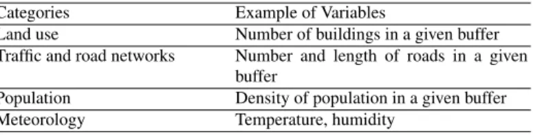
We perform a pretreatment on these data to eliminate redundant and non-significant variables. For this purpose, we first perform a Student test to eliminate the non-significant variables. We calculate then the variance inflation factor (VIF) in order to check whether the information provided by a variable is present in one or more other variables of the model. We eliminate variables with a high VIF in order to reduce multicollinearity. Finally, we calculate the adjusted R2, which evaluates the contribution of each variable to the model, before and after adding each variable and then we eliminate the non-significant variables to the model. Following these steps, we validated around 35 % of the initial variables. We divided the resulting variables into four categories listed in table 2:

Table 2 Main categories of dependant variables

Categories Example of Variables

Land use Number of buildings in a given buffer Traffic and road networks Number and length of roads in a given

buffer

Population Density of population in a given buffer Meteorology Temperature, humidity

5 Performance evaluation

We compare in this section different mapping strategies while taking into consideration the intrinsic char-acteristics of dense deployment of low cost WSN for air quality monitoring. We first evaluate and

com-1_{https://data.grandlyon.com/}

2_{https://donneespubliques.meteofrance.fr/} 3_{https://earthexplorer.usgs.gov/}

pare some regression approaches regarding different metrics and conduct after that comparisons against the BLUE assimilation method.

5.1 Choice of the parameter k in KNN regression

The k parameter in KNN regression gives the number of the closest points to the predicted one that will be used to estimate the predicted value. On one hand, using a small k means restraining the set of a given prediction and forcing the regression to be more blind to the overall distribution. On the other hand, a higher k averages more points values and hence is more resilient to outliers. However, larger values of k will have smoother decision boundaries. To choose a good value of k, we evaluated the mean absolute error (MAE) for different values of k. The results are presented in table 3. We notice the parameter k has no significant impact on the MAE for k ∈ [3, 15]. However, the minimum MAE is reached when k=5. k is then set to 5 for the following comparisons.

Table 3 MAE vs k value of KNN regression (σm= 2 ug/m3, Fraction of deployed sensors = 0.3)

k 3 5 7 9 11 13 15 MAE 3.246 3.230 3.234 3.240 3.245 3.251 3.256

5.2 Comparing regression-based approaches in function of the fraction of deployed

sensors

We consider in this work four regression approaches: linear regression, KNN, Random forest and Xgboost. We compared these approaches on 30 realizations of ground truth obtained from a simulation with α= 0.05. First, we evaluate the behaviour of these methods regarding the MAE metric when increasing the fraction of deployed sensors. For each ground truth data set, all approaches are executed ten times with different measurement realizations (with σm=1 ug/m3). The results, depicted in Figure 3 (a), show that all methods

present a better performance when the percentage of sensors increases. Indeed the more sensors are deployed, the lowest the error is and the better the estimate is. Random forest outperforms all the methods reaching an MAE of 1.48 ug3when 40% of sensors are deployed, it is followed nearly by xgboost and then KNN and linear regression.

5.3 Impact of sensor errors on regression methods

In order to assess the impact of sensing errors and the high density on the behaviour of the regression methods, we evaluate these methods regarding the fraction of deployed nodes with different sensing errors. For that, we plot in Figure 3 (b) the MAE of the Xgboost method, considering three different sensing standard deviation error (σm= 1, 3 and 7 ug/m3) while varying the percentage of deployed sensors. The results show

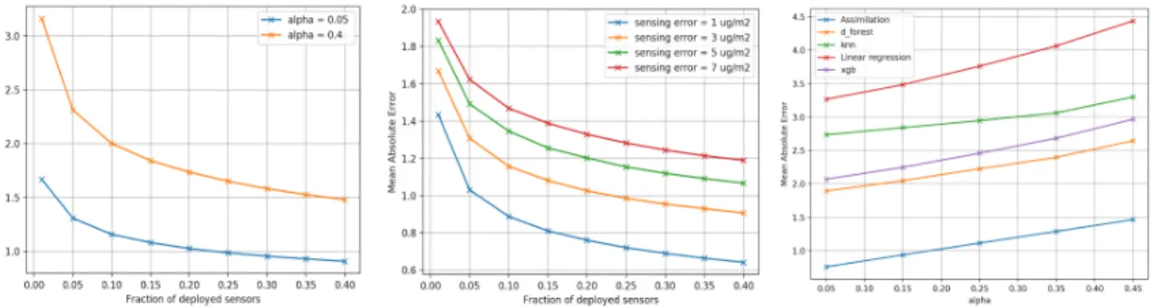
Fig. 3 (a) MAE Vs percentage of deployed sensors, σm= 1 ug/m3; (b) MAE of Xgboost method Vs percentage of deployed

sensors,s ∈ [1, 3, 7]; (c) MAE Vs Standard error deviation, Fraction of deployed sensors = 0.3

that when the error of sensing is relatively high (>=3), increasing the number of deployed sensors does not necessarily improve the results, but instead decreases the performances when the density exceeds an optimal sensor density. In this case, when the sensors have a significant measurement error it is not interesting to deploy more sensors to improve the performance. The results of the four regression approaches are similar with different sensing error threshold and different optimal sensor density.

In order to compare the regression methods regarding the sensing errors σm, we fixed the percentage of

deployed sensors to 30% and varied σm. Results, plotted in Figure 3 (c), show that all regression methods are

sensitive to sensor error. Indeed the MAE is higher as the sensing error increases. From the different curve slaves, we can also notice that Xgboost is less sensitive to sensing errors than random forest. Starting from a given threshold, Xgboost outperforms random forest. We also notice that linear regression is less sensitive to sensing errors compared to KNN. These results give guidelines regarding the method choice in function of the sensing errors.

5.4 Assimilation results depending on simulation errors

The data assimilation results are obtained over 30 realizations of ground truth and with different values of α increasing from 0.05 to 0.4. We recall that the higher α is, the lower is the numerical model quality. Figure 4 (a) depicts the data assimilation MAE results with two different values of α in function of the fraction of deployed sensors used to correct the model. As expected, an assimilation with an accurate simulation output (i.e. small α) performs better than an assimilation with a less accurate physical model. Moreover, the higher the fraction of deployed sensors is, the lower is the impact of the numerical model errors.

5.5 Assimilation results depending on sensing errors

To evaluate the effect of the sensing error, we perform BLUE assimilation with a fixed α (0.05) and different sensing errors σm. As illustrated in Figure 4 (b), the MAE decreases as we increase the fraction of deployed

sensors. We can observe that even with a σm=7, the assimilation still can correct the model thanks to the

Fig. 4 (a) Assimilation’s MAE Vs percentage of deployed sensors σm= 3 ug/m3; (b) Assimilation’s MAE Vs percentage of

deployed sensors, α = 0.05; (c) MAE Vs values of α, σm= 1 ug/m3, fraction of deployed sensors = 0.3

5.6 Regression Vs Assimilation

In this last simulation, we compare the different regression methods to the BLUE assimilation one with different values of α. Figure 4 (c) shows that the implemented assimilation method (BLUE) has 40% better air quality estimation compared to Random Forest which offers the best performances of regression methods. This is due to the consideration of the model’s error as well as the sensing errors in the assimilation process. BLUE performs very well when the simulation error covariance matrix and sensing error covariance matrix are well estimated.

6 Conclusions

One of the main challenges of low-cost WSN is their low accuracy. In this work, we proposed a general framework that allows the comparison of different regression and assimilation strategies based on numeri-cal simulations and an adequate estimation of the simulation error covariances as well as the sensing errors covariances. We also studied four regression approaches and one assimilation method and compared them in terms of pollution estimation quality while considering the errors of both measurements and the numer-ical model. We have shown that data assimilation is less sensitive to the variations of measurement errors. Moreover we have seen that a big number of sensors is not always good for regression methods when sen-sors present an important sensing error. However this is not the case for assimilation when numerical model errors and sensing errors are well estimated. As future research work, we intend using more realistic errors characterization by introducing some noise to R and B matrices. We also plan to extend our framework by adding new approaches and test it with real data sets.

Acknowledgements This work has been supported by the "LABEX IMU" (ANR-10-LABX-0088) of Université de Lyon, within the program "Investissements d’Avenir" (ANR-11-IDEX-0007) operated by the French National Research Agency (ANR).

References

1. World Health Organization, “Burden of disease from the joint effects of household and ambient air pollution for 2016,” 2018. [Online]. Available: https://www.who.int/airpollution/data/AP_joint_effect_BoD_results_May2018.pdf

2. P. Kumar, L. Morawska, C. Martani, G. Biskos, M. Neophytou, S. Di Sabatino, M. Bell, L. Norford, and R. Britter, “The rise of low-cost sensing for managing air pollution in cities,” Environment international, vol. 75, pp. 199–205, 2015. 3. P. Schneider, N. Castell, F. R. Dauge, M. Vogt, W. A. Lahoz, and A. Bartonova, “A network of low-cost air quality sensors

and its use for mapping urban air quality,” in Mobile Information Systems Leveraging Volunteered Geographic Information for Earth Observation. Springer, 2018, pp. 93–110.

4. P. Arroyo, J. L. Herrero, J. I. Suárez, and J. Lozano, “Wireless sensor network combined with cloud computing for air quality monitoring,” Sensors, vol. 19, no. 3, p. 691, 2019.

5. D. Hasenfratz, O. Saukh, C. Walser, C. Hueglin, M. Fierz, T. Arn, J. Beutel, and L. Thiele, “Deriving high-resolution urban air pollution maps using mobile sensor nodes,” Pervasive and Mobile Computing, vol. 16, pp. 268–285, 2015.

6. A. Anjomshoaa, F. Duarte, D. Rennings, T. J. Matarazzo, P. deSouza, and C. Ratti, “City scanner: Building and scheduling a mobile sensing platform for smart city services,” IEEE Internet of Things Journal, vol. 5, no. 6, pp. 4567–4579, 2018. 7. M. Gerboles, A. Borowiak, and L. Spinelle, “Measuring air pollution with low-cost sensors,” European Commission,

Brochure, 2017.

8. A. Boubrima, W. Bechkit, and H. Rivano, “Optimal WSN deployment models for air pollution monitoring,” IEEE Trans. Wireless Communications, vol. 16, no. 5, pp. 2723–2735, 2017.

9. A. Boubrima, W. Bechkit, and R. Hervé, “On the deployment of wireless sensor networks for air quality mapping: Opti-mization models and algorithms,” IEEE Transactions on Networking.

10. L. Soulhac, P. Salizzoni, F.-X. Cierco, and R. Perkins, “The model sirane for atmospheric urban pollutant dispersion; part i, presentation of the model,” Atmospheric Environment, vol. 45, no. 39, pp. 7379–7395, 2011.

11. L. Soulhac, P. Salizzoni, P. Mejean, D. Didier, and I. Rios, “The model sirane for atmospheric urban pollutant dispersion; part ii, validation of the model on a real case study,” Atmospheric environment, vol. 49, pp. 320–337, 2012.

12. L. Soulhac, C. V. Nguyen, P. Volta, and P. Salizzoni, “The model sirane for atmospheric urban pollutant dispersion. part iii: Validation against no2 yearly concentration measurements in a large urban agglomeration,” Atmospheric environment, vol. 167, pp. 377–388, 2017.

13. J. Kerckhoffs, M. Wang, K. Meliefste, E. Malmqvist, P. Fischer, N. A. Janssen, R. Beelen, and G. Hoek, “A national fine spatial scale land-use regression model for ozone,” Environmental research, vol. 140, pp. 440–448, 2015.

14. A. Marjovi, A. Arfire, and A. Martinoli, “Extending urban air quality maps beyond the coverage of a mobile sensor network: data sources, methods, and performance evaluation,” in EWSN, 2017.

15. A. Adam-Poupart, A. Brand, M. Fournier, M. Jerrett, and A. Smargiassi, “Spatiotemporal modeling of ozone levels in quebec (canada): a comparison of kriging, land-use regression (lur), and combined bayesian maximum entropy–lur ap-proaches,” Environmental health perspectives, vol. 122, no. 9, pp. 970–976, 2014.

16. M. Bocquet, H. Elbern, H. Eskes, M. Hirtl, R. Žabkar, G. Carmichael, J. Flemming, A. Inness, M. Pagowski, J. Pérez Ca-maño et al., “Data assimilation in atmospheric chemistry models: current status and future prospects for coupled chemistry meteorology models,” Atmospheric chemistry and physics, vol. 15, no. 10, pp. 5325–5358, 2015.

17. A. Tilloy, V. Mallet, D. Poulet, C. Pesin, and F. Brocheton, “Blue-based no 2 data assimilation at urban scale,” Journal of Geophysical Research: Atmospheres, vol. 118, no. 4, pp. 2031–2040, 2013.

18. U. Kumar, K. De Ridder, W. Lefebvre, and S. Janssen, “Data assimilation of surface air pollutants (o3 and no2) in the regional-scale air quality model aurora,” Atmospheric environment, vol. 60, pp. 99–108, 2012.

19. X. Wang, V. Mallet, J.-P. Berroir, and I. Herlin, “Assimilation of omi no2 retrievals into a regional chemistry-transport model for improving air quality forecasts over europe,” Atmospheric environment, vol. 45, no. 2, pp. 485–492, 2011. 20. X. Xie, I. Semanjski, S. Gautama, E. Tsiligianni, N. Deligiannis, R. Rajan, F. Pasveer, and W. Philips, “A review of urban air

pollution monitoring and exposure assessment methods,” ISPRS International Journal of Geo-Information, vol. 6, no. 12, p. 389, 2017.

21. M. Jerrett, M. Arain, P. Kanaroglou, B. Beckerman, D. Crouse, N. Gilbert, J. Brook, N. Finkelstein, and M. Finkelstein, “Modeling the intraurban variability of ambient traffic pollution in toronto, canada,” Journal of Toxicology and Environ-mental Health, Part A, vol. 70, no. 3-4, pp. 200–212, 2007.

22. T. Chen, T. He, M. Benesty, V. Khotilovich, and Y. Tang, “Xgboost: extreme gradient boosting,” R package version 0.4-2, pp. 1–4, 2015.

23. G. Biau, “Analysis of a random forests model,” Journal of Machine Learning Research, vol. 13, no. Apr, pp. 1063–1095, 2012.