HAL Id: insu-02395300
https://hal-insu.archives-ouvertes.fr/insu-02395300
Submitted on 8 Mar 2021HAL is a multi-disciplinary open access archive for the deposit and dissemination of sci-entific research documents, whether they are pub-lished or not. The documents may come from teaching and research institutions in France or abroad, or from public or private research centers.
L’archive ouverte pluridisciplinaire HAL, est destinée au dépôt et à la diffusion de documents scientifiques de niveau recherche, publiés ou non, émanant des établissements d’enseignement et de recherche français ou étrangers, des laboratoires publics ou privés.
Optimization of ion trajectories in a dynamically
harmonized Fourier-Transform Ion Cyclotron Resonance
cell using a Design of Experiments strategy
Julien Maillard, Justine Ferey, Christopher P. Rüger, Isabelle Schmitz-Afonso,
Soumeya Bekri, Thomas Gautier, Nathalie Carrasco, Carlos Afonso, Abdellah
Tebani
To cite this version:
Julien Maillard, Justine Ferey, Christopher P. Rüger, Isabelle Schmitz-Afonso, Soumeya Bekri, et al.. Optimization of ion trajectories in a dynamically harmonized Fourier-Transform Ion Cyclotron Resonance cell using a Design of Experiments strategy. Rapid Communications in Mass Spectrometry, Wiley, 2020, 34 (7), pp.e8659. �10.1002/rcm.8659�. �insu-02395300�
1
Optimization of ion trajectories in a dynamically
1
harmonized Fourier-Transform Ion Cyclotron
2
Resonance cell using a Design of Experiments
3
strategy
4 5
Julien MAILLARD1,2, Justine FEREY2, Christopher P. Rüger2, Isabelle SCHMITZ-6
AFONSO2, Soumeya BEKRI3, Thomas GAUTIER1, Nathalie CARRASCO1, Carlos 7
AFONSO2 and Abdellah TEBANI2.3* 8
9
1LATMOS/IPSL, Université Versailles St Quentin, UPMC Université Paris 06, CNRS, 11 10
blvd d’Alembert, F-78280 Guyancourt, France
11
2 Université de Rouen, Laboratoire COBRA UMR 6014 & FR 3038, IRCOF, 1 Rue 12
Tesnière, 76821 Mont St Aignan Cedex, France 13
3 Department of Metabolic Biochemistry, Rouen University Hospital, Rouen, 76000, 14
France 15
2
Abstract
17
The optimization of the ion trajectories in the ion cyclotron resonance (ICR) cell of a 18
Fourier transform ICR mass spectrometer is a crucial step to obtain the best dynamic range, 19
mass resolution, and mass accuracy. With the recent introduction of the dynamically 20
harmonized cell, the complexity of tuning expanded drastically, and a fine-tuning of the 21
DC voltages is required to optimize the ion cloud movement. This adjustment is typically 22
performed manually. 23
Here, we propose a computational method based on a design of experiments (DoE) strategy 24
to overcome the limits of classical manual tuning. This DoE strategy was exemplarily 25
applied on a 12T FTICR equipped with a dynamically harmonized ICR cell. The 26
chemometric approach, based on a composite central face design (CCF), was first applied 27
on a reference material (sodium trifluoroacetate) allowing for the evaluation of the primary 28
cell parameters. Eight factors were identified related to shimming and gating. The summed 29
intensity of the signal corresponding to the even harmonics was defined as one quality 30
criteria. 31
Consequently, the DoE response allowed for rapid and complete mapping of cell 32
parameters resulting in an optimized parameter set. The new set of cell parameters was 33
applied to the study of an ultra-complex sample. Here, Tholins, an ultra-complex mixture 34
that mimics the haze present on Titan, was chosen. We observed a substantial improvement 35
in mass spectrometric performance. The sum of signals related to harmonics was decreased 36
by a factor of three (from 4% for conventional tuning to 1.3%). Furthermore, the dynamic 37
range was also increased and lead to an increase of attributed peaks by 13%. 38
3
Graphical abstract
39
40 41
4
1. Introduction
42
Fourier Transform Ion Cyclotron Resonance mass spectrometer (FTICR) is well known to 43
be the most powerful mass spectrometer by reaching unprecedented resolving power, mass 44
accuracy and sensitivity levels1,2. It turned out to be the most appropriate instrument for the 45
characterization of ultra-complex mixtures such as petroleum3-7, natural organic matter 8 or 46
extraterrestrial organic matter 9,10. In order to detect the cyclotron motion, FTICR uses the 47
combination of a static electric field which is hyperbolic near the center and a strong 48
homogeneous static magnetic field (up to 21 Tesla – so far). The combination of both fields 49
retains ions in the cell. Ions in the magnetic field travel according to a cyclotron motion 50 defined by equation 1. 51 𝜔0 = 𝑞𝐵0 𝑚 52
Equation 1: Cyclotron frequency (ω0) of a charged particle in a homogeneous magnetic 53
field. q is the charge of the particle, B0 the strength of the magnetic field and m the mass of 54
the particle. 55
56
In addition, the ion packet undergoes a drift of a trajectory equal to ExB where E is the 57
electric field and B is the magnetic field. Both of these movements allow the ion packet to 58
be trapped in the cell2,11. 59
The shape of the ICR cell was improved steadily over time from first cubic geometry12 to 60
a variety of spherical designs varying in electrode shape and number 13. As an example, the 61
orthorhombic capacitively coupled cell developed by Steven Beu in 1991 14 or the infinity 62
cell which was designed by Caravatti et al. in 1991 are cited here 15, the later remaining the 63
most commonly used nowadays . In recent instruments, the so-called dynamically 64
harmonized cell is frequently deployed 2. For the purpose of radiofrequency excitation and 65
detection of ions, the cell is composed of several electrodes. In case of the dynamically 66
5
harmonized cell, these excitation and detection electrodes are specially shaped to 67
compensate the quadrupolar electric field over the entire cell’s body. It allows to produces 68
a volume where, over the orbit of the ions, the average field is quadrupolar at all cyclotron 69
radii. Thus, the frequency drifts of ions of the same mass over time along the Z axis are 70
reduced. This makes possible to record transients for a longer time than in the previous 71
cells and thus significantly improve performance 72
Optimized detection in terms of highest resolving power, sensitivity and dynamic range is 73
obtained when the ion cloud is perfectly centered in the middle of the magnet. However, in 74
practice, the imperfections of the alignment cause a bias in the position of the ion packets 75
and thus a deviation in the cyclotron motion synchronization. This issue is solved by adding 76
another set of segments to the dynamically harmonized cell in order to smooth 77
imperfections by applying additional DC (Direct Current) voltages 11. With this approach, 78
it is possible to decrease the abundance of even-harmonic signals and, thus, to minimize 79
magnetron motion. However, the values for the additionally applied DC voltages have to 80
be tuned manually, which requires specially trained personnel and is tedious and time-81
consuming. In the present work, an experimental design approach is proposed in order to 82
overcome the drawbacks of the manual ICR cell tuning. The approach seeks to optimize 83
the DC voltages and reach the best set of parameters. Design of experiments (DoE) is a 84
rigorous procedure in which defined modifications are induced based on a given set of 85
variables. The response of the system is recovered to create a mathematical model, which 86
allows a prediction of a set of parameters optimizing the response value16-18. Some example 87
of mass spectrometer’s optimization using DoE can be cite, such as the work performed by 88
Lemonakis et al (2016) and Tebani et al (2016) 19,20. Here, this method is applied on a 89
defined response, the sum of the abundance of the second harmonic of sodium 90
trifluoroacetate cluster. 91
6
After optimization, the obtained parameters are applied to the analysis of a complex 92
mixture, Tholins. This synthetic material is used to understand the chemistry occurring in 93
Titan’s atmosphere by artificially mimicking the brown haze surrounding the largest moon 94
of Saturn21-25. More importantly, Tholins have shown to be ultra-complex mixtures with 95
high isobaric complexity and thousands of elemental compositions 26. Tholins spectra 96
obtained after DoE and after the usual manual method are compared. The potential of the 97
developed method for complex mixtures analysis is highlighted evaluating the mass 98
spectrometric performance, i.e., resolving power, the abundance of harmonics and number 99
of detected signals. 100
7
2. Experimental methods
102
2.1. Tholins production
103
Tholins were produced following the PAMPRE procedure (French acronym for Aerosols 104
Microgravity Production by Reactive Plasmas) presented elsewhere24,27. Briefly, in a 105
stainless steel tubular reactor, a continuous gas mixture composed of 95 v-% nitrogen and 106
5 v-% methane was injected through polarized electrodes and evacuated by a primary 107
vacuum pump system. A Radio Frequency – Capacity Coupled Plasma (RF-CCP) 108
discharge was established in the gas mixture deploying an RF of 13.56 MHz. The pressure 109
in the plasma discharge was maintained at 0.9 ± 0.1 mbar, and the reaction took place at 110
room temperature (293 K). 111
2.2. Instrumentation
112
2.2.1. Fourier transform ion cyclotron resonance mass spectrometer
113
All analyses were performed on a FTICR Solarix XR from Bruker equipped with a 12T 114
superconducting magnet and a dynamically harmonized ICR cell. The following ion 115
transfer parameters were used for both electrospray (ESI) and laser desorption ionization 116
(LDI) analyses in positive ion mode: capillary exit 150V, deflector plate 200V, funnel1 117
150V, skimmer1 25V, funnel RF amplitude 60Vpp, octopole frequency 5MHz, octopole 118
RF amplitude 350Vpp, lower cut-off of the quadrupole at m/z 120, time-of-flight 0.7ms, 119
frequency TOF 6MHz, TOF RF amplitude 200Vpp, side kick offset -1V, front and back 120
trapping plate 1.75V. 121
For ESI the following parameters were used: capillary 4.5kV, spray shield -500V, dry gas 122
flow 2L.min-1, dry gas temperature 180°C, nebulizer gas flow 0.5bar. All analyses were 123
recorded on 20 scans with a quadrupole accumulation time of 0.1s. Electrospray spectra 124
8
were recorded with a mass range from m/z 98 to 1,200 and a transient length of 2.2s. Sodium 125
trifluoroacetate (NaTFA, Sigma Aldrich) at 0.1mg.ml-1 in ACN/H
2O (50/50, v/v) was used 126
as a standard for the design of experiments approach. 127
Complex Tholins mixture analyses was recorded applying LDI. The solid sample was 128
deposed on a MALDI plate following previous work28. The third harmonic of a Nd:YAG 129
laser at 355nm delivering a maximum output of 0.5mJ (Smartbeam II, Bruker) was used to 130
ionize the samples with the following parameters: laser power 15%, laser shots per scan 131
50, shots frequency 1kHz, plate offset 100V. The recorded mass spectra combined 800 132
scans to achieve high signal-to-noise. LDI spectra were recorded with a mass range from 133
m/z 110 to 1200 and a transient length of 4.3s.
134
2.3. Experimental design
135
2.3.1. Software
136
DataAnalysis 4.4 (Bruker Daltonics GmbH, Bremen) was used to process all mass 137
spectrometric analyses, including m/z-calibration and response recovering (abundance of 138
the harmonic signals). 139
MODDE 11 software (Umetrics, Sartorius Stedim Data Analytics AB, Umea, Sweden) was 140
used to perform the consecutive data analyses and modeling. The initial step is the 141
definition of the response (i.e., user observation). Then, in a second step, factors influencing 142
the response are defined. Afterward, several choices of experimental design shapes can be 143
chosen. The software will automatically create the DoE given to the user as a coded matrix 144
(Table 1) and a real matrix (Table S1). This matrix defines the experiments to be recorded 145
and from which the response has to be extracted. Then, MODDE propose an automatic 146
fitting method (e.g., partial least squares regression - PLS) allowing the visualization of the 147
9
quality and the predictability of the DoE. Finally, the optimizer tool was used to predict the 148
set of parameters giving the best response result. 149
2.3.2. Factorial designs
150
The tuning of the ICR cell is established with eight principal parameters, four shimming 151
parameters (shimming 0°, shimming 180°, shimming 90° and shimming 270°) and four 152
gating settings (gated 0°, 90°, 180°, and 270°)11. The set of gating parameters represents 153
the values of DC voltages applied during the injection in the ICR cell in order to correctly 154
trap the ion packets. The set of shimming parameters represents the values of DC voltages 155
applied for the excitation and the detection of the ions packets in the ICR cell. A simplified 156
description of the ICR cell is given in figure 1. Other parameters of the ICR cell are not 157
included (e.g., back and front plate voltages, sidekick offset) as they are easily and rapidly 158
manually tunable. This significantly reduces the number of experiments required for the 159
DoE approach, considerably decreasing the optimization time. 160
Parameters were grouped in pairs leading to four couples of parameters: shimming 0°-180° 161
(Shi0), shimming 90°-270° (Shi90), gated 0°-180° (Gat0) and gated 90°-270° (Gat90) 162
simplifying the optimization process compared to the conventional manual procedure. The 163
values of these couples change symmetrically, meaning that when the value of one part is 164
increased, the other part decreases about the same value. Initially, all values are set to 1.5V 165
(default settings). As example, increasing the value of the shimming 0° about 50mV to 166
1.55V results at a value of the shimming 180° of 1.45V. In addition to these four coupled 167
parameters, the sweep excitation power (SEP) was added as a factor parameter for the first 168
step of the optimization strategy. SEP has a crucial impact on the ion trajectories as it 169
defines their radius. After defining the assessed experimental factors, it was necessary to 170
define the desired response as a result of the optimization. Following the classical 171
10
optimization method, the intensity ratio between the ion of the NaTFA at m/z 702.86324 172
and its second harmonic at m/z 351.43164 was recovered. 173
The optimization of the dynamically harmonized cell parameters was divided into two 174
steps. The first screening step was performed with wide parameter intervals to evaluate the 175
effects of each parameter on the defined response. The second part, named optimization 176
experimental design, focused on narrower intervals to reach the best set of parameters. The 177
applied chemometric approach for the two steps is based on a Composite Central 178
Composite face design (CCF) which takes into account interactions between parameters. 179
The coded CCF for the first step is given in Table 1 formatted according to the required 180
software input. Basically, the table reflects the conducted experimental plan, where -1 181
means that the parameter was set at the respective low level (e.g., for Shi 0 at 1.465V) and 182
+1 at the respective high level. Defined intervals for each parameter are given in Table 2 183
for the screening and optimization step. These intervals have been defined quickly by 184
varying each of the parameters until the intensity of the harmonic reaches a minimum level. 185
This step takes about 5 minutes. 186
2.3.3. Multivariate modeling
187
Partial Least Squares regression (PLS) was used to model each CCF design and to find the 188
best set of parameters regarding the response chosen using the optimizer tool implemented 189
in MODDE 11. Thus, PLS coefficients are used to estimate factor effects. A positive value 190
of the coefficient indicates an increase of the response upon increasing the corresponding 191
parameter, whereas a negative value indicates a decrease of the response upon increasing 192
the corresponding parameter. The larger the absolute value of the PLS coefficient, the 193
higher the effect of the parameter on the response. Analysis of variance (ANOVA) applied 194
to the sum of squares of the PLS regression coefficient was used to assess the significance 195
11
of the factor effect. For a statistically significant effect of a factor, the model p-value of 196
ANOVA should not exceed 0.0529. 197
3. Results and discussion
198
3.1. Screening experimental design using NaTFA
199
The design of experiments approach was performed using NaTFA to minimize the 200
abundance of signals related to harmonics. Briefly, the influence of four pairs of factors 201
and the SEP (Shi0, Shi90, Gat0, Gat90, and Sweep Excitation Power) was evaluated using 202
an even harmonic peak intensity of the ion m/z 702.86324 at m/z 351.43164 as the response. 203
A Central Composite Face design (CCF) was chosen as it is generally applicable for this 204
type of optimization problems. 205
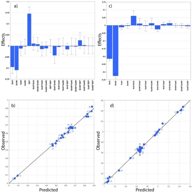
Figure 2a visualizes the effect of the different factors on the even harmonic abundance in
206
the screening step. SEP, Shi0, and Shi90 revealed the most significant effects on the 207
intensity of the second harmonic peak, with contribution factors of 28.0%, 15.4%, and 208
33.3% respectively. SEP played a positive effect with high values leading to high 209
abundance of the harmonic. In contrast, Shi0 and Shi90 showed a negative response, with 210
high values resulting in low abundance of the harmonic. In addition, the interaction of Shi0 211
and Shi90 provided a significant positive effect, which is related to a high separation effect 212
of these parameters. Hence these two couples of parameters have two very different effects 213
on the abundance of the harmonic and, thus, on the ion cloud trajectories. 214
The prediction plot obtained based on the 27 experimental data points, between the 215
predicted and observed values of the abundance of the second harmonic, is shown in Fig. 216
2b. This representation allows to access the quality of prediction with this model based on
217
the initial data set. The cumulative modeled variation (R²X = 99.1%) and the cumulative 218
predicted variation (Q²Y = 62.8%) reflect the explained variance and the predictability of 219
12
the model. The near to one R2X value proves the validity of the model. The Q2Y value 220
(which is above 50%) proves that the model can give predictable values of parameters for 221
the defined response 17,18,29. However, this value could be improved to obtain better 222
optimization results, which will be the aim of the following part of the optimization 223
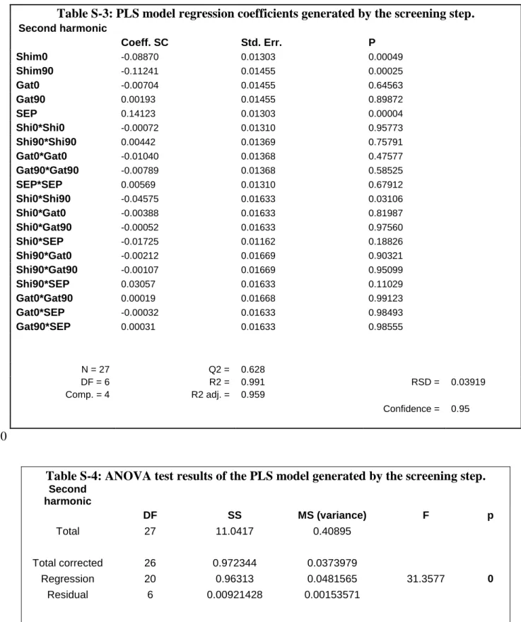
experimental design. The values of the regression coefficients and their respective p-values 224
are given in Table S-3 (Supplementary data). The fitted models’ metrics, ANOVA and 225
validation results of each model are presented in Tables S-4 and S-5 (Supplementary data). 226
Using this built model, the instrumental parameters were optimized to reach the lowest 227
harmonic intensity. The predicted optimized values are presented in Table 2. Nevertheless, 228
the obtained set of predicted values reach the extremity of each defined interval. Therefore, 229
an additional optimization step was performed focusing on tight intervals for Shi0, Shi90, 230
Gat0, and Gat90. It should be noted that the SEP and shimming values are two decorrelated 231
parameters. In the rest of this study, the SEP was fixed at a value of 30% in order to focus 232
on fine tuning. This value is a percentage of the maximum excitation amplitude. 233
3.2. Optimization experimental design using NaTFA
234
As described above, for this step, the sweep excitation power (SEP) was removed from the 235
studied factors to focus only on the cell parameters. It turned out, that Shi0 and Shi90 had 236
a major negative response on the second harmonic abundance (Fig. 2c), which is consistent 237
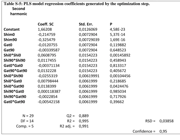
with the results obtained in the previous screening step. Coded regression coefficients, 238
ANOVA and model validation results are given in Tables S-2, S-5, and S-6 239
(Supplementary data). The fitted model shows a cumulative modeled variation of R2X = 240
99.5% and a cumulative predicted variation of Q2Y = 88.9% as showed in Fig. 2d. These 241
results improved compared to the screening step and proved the high predictability of the 242
movement of ions in the dynamically harmonized cell. Using this built model, the 243
13
optimized set of parameters provided an abundance of 1.3% of second harmonics compared 244
to the base signal. In comparison, the non-optimized parameters (manufacturer default 245
values) provided 8% and manually optimized parameters provided 4% of harmonic 246
abundance, respectively. 247
This first study proved the possible optimization of the movement of ions in the ICR cell 248
by lowering harmonic peaks. This DoE methodology was validated by the study of a 249
NaTFA standard solution typically used for instrument calibration and optimization. 250
However, the high interest of optimizing the ion trajectories in the ICR cell is related to the 251
description of complex mixtures with unknown constituents. Consequently, the set of 252
parameters yielded by the DoE methodology have been applied to study Titan tholins. The 253
results were compared to those obtained after the manual optimization. 254
3.3. Application for the analysis of complex mixtures: Titan tholins
255
The largest moon of Saturn, Titan, is surrounded by a thick and nitrogen-rich fog with some 256
fraction of methane30-33. Understanding how this haze is produced along with its molecular 257
composition are crucial steps from a planetary and prebiotic chemistry perspective34,35. 258
Tholins are analogs of Titan’s haze. They are laboratory-produced and used as a proxy on 259
Earth as there is currently no sample return option. This material is an extremely complex 260
mixture comparable to the complexity of petroleum and as such ideal for evaluating the 261
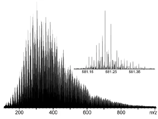
tuning of the dynamically harmonized cell parameters26. Figure 3 shows an overview of a 262
tholins mass spectrum, containing more than 50,000 peaks. This mass spectrum was 263
generated with LDI ionization together with the optimized cell tuning parameters resulting 264
from the DoE approach on NaTFA. The insert in Figure 3 presents the molecular 265
complexity on a single nominal mass revealing more than 100 resolved peaks. In this study, 266
14
we used this ultra-complex sample to compare the effects of the above-described 267
optimization strategy with the conventional method relying on manual optimization. 268
The comparison between the detected species applying the parameters given by manual 269
tuning and DoE optimization is illustrated in Figure 4. The mass spectrum at the top was 270
recorded after the conventional manual optimization of the ICR cell. This manual 271
optimization can take several hours easily to obtain high performance due to the manual 272
iteration process. The spectrum at the bottom was recorded after deploying the optimized 273
parameter set given by the newly developed DoE strategy, which takes approximately one 274
hour. It should be mentioned that the shimming parameters are re-optimized once a year to 275
compensate instrumental’s drift. Except for the cell parameters, the two spectra were 276
recorded with the exact same conditions. The number of detected species is significantly 277
higher with the DoE optimization. Figure 4, giving a small fraction of the mass 278
spectrometric complexity revealed thirteen additional species (indicated with a red star) for 279
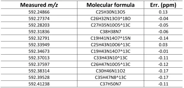
the DoE optimized spectrum compared to the spectrum resulted after manual tuning. The 280
attribution of these new peaks is given in table S-7. This observation can be induced by 281
two effects: 1) The ion packets is more centered in the cell thanks to the computational 282
method, inducing a higher dynamic range or, 2) in the spectrum after manual adjustment, 283
some peaks are in coalescence with their close neighbor. This effect is not present after the 284
DoE tuning, which explain why more peaks are observed in this case. In order to reinforce 285
this, through attributions, it can be justified that these peaks are not harmonics. Manual 286
optimization is a difficult and limited process. Indeed, it is impossible for the human eye to 287
take into account the interactions between the various parameters.Therefore, the location 288
of the ions is not perfectly centered and could still be improved. Furthermore, this method 289
is a time-consuming iterative process based on trial and error steps to reach acceptable 290
values specified by the manufacturer (here below 6% for the second harmonic). The above 291
15
described DoE strategy, performed with NaTFA, allows a complete mapping of the 292
different parameter effects along with their interactions, which allows modeling of the 293
system. Thus, this strategy leads to a more fine-tuning and a greater reduction of harmonics 294
compared to the conventional manual attempt. 295
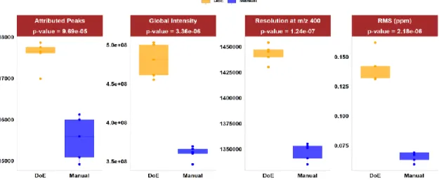
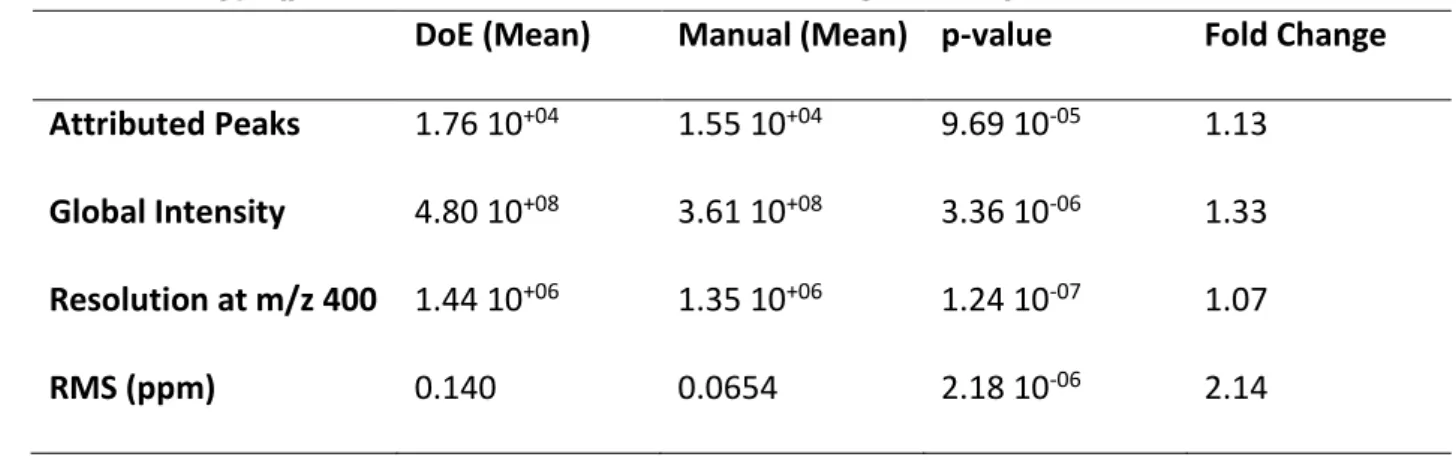
Different metrics obtained for DoE originated and manually recorded spectra are listed in 296
Table 3. These results were obtained after recording 5 replicates for each tuning. As
297
illustrated in Figure 4 applying the DoE generated parameters significantly increased the 298
number of observed peaks. The comparison with the manually tuned cell revealed 13% 299
more peaks attributed after the DoE tuning. The resolving power is also slightly increased 300
after the experimental design optimization: approx. 1,440,000 with the DoE method and 301
1,350 000 with the manual method at m/z 400. A slight increase is also observed for the 302
average mass accuracy of the elemental composition assignment. All these results are 303
summarized in Figure 5. 304
The application of the new predicted dynamically harmonized cell parameters on Titan’s 305
tholins showed a clear enhancement on almost every metric of the recorded spectrum in 306
comparison with the spectrum generated with the non-tuned cell but also with the manually 307
tuned cell. Furthermore, this work will be useful for the implementation of quadrupolar ion 308
detection, which commonly induces higher order harmonics with increased abundance. 309
This newly developed optimization strategy is highly time efficient compared to the 310
conventional method, taking only one hour including the recording of the spectra, data 311
processing, and data analysis.It is a universal approach and can be applied to any complex 312
mixture such as petroleum and biological sample materials. Those ultra-complex mixtures 313
usually raises high analytical challenges regarding experimental optimization. 314
16
4. Conclusions
316
The developed design of experiments (DoE) strategy has proven to be applicable for 317
generating optimized parameter sets for a dynamically harmonized ICR cell. We could 318
show that the approach results in settings leading to a reduction of harmonics to levels not 319
reached by manual tuning and far below the manufacturer default values. Moreover, the 320
optimization process takes significantly less time and can be performed by any instrument 321
user. This substantial improvement allows for a better performance of the FTICR by 322
significantly increasing all metrics of the recorded spectrum, i.e., mass accuracy, resolution 323
and dynamic range, for both the standard as well as the ultra-complex mixture. Finally, this 324
computational procedure based on a composite face design could be applied for any other 325
mass spectrometric parameter optimization problem. The authors believe this will allow for 326
a more transparent and more structured design when performing method development. 327
328
17
5. Acknowledgments
330
N.C. thanks the European Research Council for funding via the ERC PrimChem project 331
(grant agreement No. 636829.). 332
Financial support from the National FT-ICR network (FR 3624 CNRS) for conducting the 333
research is also gratefully acknowledged. 334
This work was also supported at COBRA laboratory by the European Regional 335
Development Fund (ERDF N°31708), the Région Normandie, and the Labex SynOrg 336
(ANR-11-LABX-0029) together with Normandie Université (NU), the Centre National de 337
la Recherche Scientifique (CNRS), Université de Rouen Normandie (URN) and Innovation 338
Chimie Carnot (I2C). 339
18
6. References
341
1. Smith RD, Cheng X, Bruce JE, Hofstadler SA, Anderson GA. TRAPPING, 342
DETECTION AND REACTION OF VERY LARGE SINGLE MOLECULAR-343
IONS BY MASS-SPECTROMETRY. Nature. 1994;369(6476):137-139. 344
2. Nikolaev EN, Boldin IA, Jertz R, Baykut G. Initial experimental characterization 345
of a new ultra-high resolution FTICR cell with dynamic harmonization. Journal of 346
the American Society for Mass Spectrometry. 2011;22(7):1125-1133.
347
3. McKenna AM, Purcell JM, Rodgers RP, Marshall AG. Heavy Petroleum 348
Composition. 1. Exhaustive Compositional Analysis of Athabasca Bitumen HVGO 349
Distillates by Fourier Transform Ion Cyclotron Resonance Mass Spectrometry: A 350
Definitive Test of the Boduszynski Model. Energy & Fuels. 2010;24(5):2929-2938. 351
4. Smith DF, Podgorski DC, Rodgers RP, Blakney GT, Hendrickson CL. 21 Tesla FT-352
ICR Mass Spectrometer for Ultrahigh-Resolution Analysis of Complex Organic 353
Mixtures. Analytical chemistry. 2018;90(3):2041-2047. 354
5. Rodgers RP, McKenna AM. Petroleum analysis. Analytical chemistry. 355
2011;83(12):4665-4687. 356
6. Hughey CA, Rodgers RP, Marshall AG. Resolution of 11 000 Compositionally 357
Distinct Components in a Single Electrospray Ionization Fourier Transform Ion 358
Cyclotron Resonance Mass Spectrum of Crude Oil. Analytical chemistry. 2002;74. 359
7. Marshall AG, Rodgers RP. Petroleomics: chemistry of the underworld. Proceedings 360
of the National Academy of Sciences of the United States of America.
361
2008;105(47):18090-18095. 362
8. Li L, Fang Z, He C, Shi Q. Separation and characterization of marine dissolved 363
organic matter (DOM) by combination of Fe(OH)3 co-precipitation and solid phase 364
extraction followed by ESI FT-ICR MS. Analytical and bioanalytical chemistry. 365
2019;411(10):2201-2208. 366
9. Schmitt-Kopplin P, Gabelica Z, Gougeon RD, et al. High molecular diversity of 367
extraterrestrial organic matter in Murchison meteorite revealed 40 years after its 368
fall. Proceedings of the National Academy of Sciences of the United States of 369
America. 2010;107(7):2763-2768.
370
10. Schmitt-Kopplin P, Harir M, Kanawati B, Tziozis D, Hertkorn N, Gabelica Z. 371
Chemical footprint of the solvent soluble extraterrestrial organic matter occluded in 372
soltmany ordinary chondrite. Meteorites. 2012:79-92. 373
11. Jertz R, Friedrich J, Kriete C, Nikolaev EN, Baykut G. Tracking the Magnetron 374
Motion in FT-ICR Mass Spectrometry. Journal of the American Society for Mass 375
Spectrometry. 2015;26(8):1349-1366.
376
12. Guan S, Marshall AG. Ion traps for Fourier transform ion cyclotron resonance mass 377
spectrometry: principles and design of geometric and electric configurations. 378
International Journal of Mass Spectrometry and Ion Processes.
1995;146-147:261-379
296. 380
13. Marshall AG, Hendrickson CL, Jackson GS. Fourier transform ion cyclotron 381
resonance mass spectrometry: A primer. Mass Spectrometry Reviews. 382
1998;17(1):1-35. 383
14. Beu SC, Laude DA. Open trapped ion cell geometries for Fourier transform ion 384
cyclotron resonance mass spectrometry. International Journal of Mass 385
Spectrometry and Ion Processes. 1992;112(2-3):215-230.
19
15. Caravatti P, Allemann M. The ‘infinity cell’: A new trapped-ion cell with 387
radiofrequency covered trapping electrodes for fourier transform ion cyclotron 388
resonance mass spectrometry. Organic Mass Spectrometry. 1991;26(5):514-518. 389
16. Gerretzen J, Szymanska E, Jansen JJ, et al. Simple and Effective Way for Data 390
Preprocessing Selection Based on Design of Experiments. Analytical chemistry. 391
2015;87(24):12096-12103. 392
17. Eliasson M, Rannar S, Madsen R, et al. Strategy for optimizing LC-MS data 393
processing in metabolomics: a design of experiments approach. Analytical 394
chemistry. 2012;84(15):6869-6876.
395
18. Eriksson L. Design of Experiments: Principles and Applications 396
Umetrics. 2008.
397
19. Lemonakis N, Skaltsounis AL, Tsarbopoulos A, Gikas E. Optimization of 398
parameters affecting signal intensity in an LTQ-orbitrap in negative ion mode: A 399
design of experiments approach. Talanta. 2016;147:402-409. 400
20. Tebani A, Schmitz-Afonso I, Rutledge DN, Gonzalez BJ, Bekri S, Afonso C. 401
Optimization of a liquid chromatography ion mobility-mass spectrometry method 402
for untargeted metabolomics using experimental design and multivariate data 403
analysis. Analytica chimica acta. 2016;913:55-62. 404
21. Khare BN, Sagnan C, Zumberge JE, Sklarew DS, Nagy B. Organic Solids Produced 405
by Electrical Discharge in Reducing Atmospheres Tholin Molecular Analysis. 406
Icarus. 1981;48:290-297.
407
22. Coll P, Coscia D, Smith N, et al. Experimantal laboratory simulation of Titan's 408
atmosphere: aerosols and gas phase. Planetary and Space Science. 1999;47:1331-409
1340. 410
23. Somogyi A, Oh CH, Smith MA, Lunine JI. Organic environments on Saturn's 411
moon, Titan: simulating chemical reactions and analyzing products by FT-ICR and 412
ion-trap mass spectrometry. Journal of the American Society for Mass 413
Spectrometry. 2005;16(6):850-859.
414
24. Szopa C, Cernogora G, Boufendi L, Correia JJ, Coll P. PAMPRE: A dusty plasma 415
experiment for Titan's tholins production and study. Planetary and Space Science. 416
2006;54(4):394-404. 417
25. Imanaka H, Smith MA. Formation of nitrogenated organic aerosols in the Titan 418
upper atmosphere. Proceedings of the National Academy of Sciences. 2010;107. 419
26. Maillard J, Carrasco N, Schmitz-Afonso I, Gautier T, Afonso C. Comparison of 420
soluble and insoluble organic matter in analogues of Titan's aerosols. Earth and 421
Planetary Science Letters. 2018;495:185-191.
422
27. Gautier T, Carrasco N, Buch A, Szopa C, Sciamma-O’Brien E, Cernogora G. Nitrile 423
gas chemistry in Titan’s atmosphere. Icarus. 2011;213(2):625-635. 424
28. Barrere C, Hubert-Roux M, Lange CM, et al. Solvent-based and solvent-free 425
characterization of low solubility and low molecular weight polyamides by mass 426
spectrometry: a complementary approach. Rapid communications in mass 427
spectrometry : RCM. 2012;26(11):1347-1354.
428
29. Montgomery D. Design and Analysis of Experiments. John Wiley & Sons. 2008. 429
30. Niemann HB, Atreya SK, Bauer SJ, et al. The abundances of constituents of Titan's 430
atmosphere from the GCMS instrument on the Huygens probe. Nature. 431
2005;438(7069):779-784. 432
31. Fulchignoni M, Ferri F, Angrilli F, et al. In situ measurements of the physical 433
characteristics of Titan's environment. Nature. 2005;438(7069):785-791. 434
20
32. Lebreton JP, Witasse O, Sollazzo C, et al. An overview of the descent and landing 435
of the Huygens probe on Titan. Nature. 2005;438(7069):758-764. 436
33. Israel G, Szopa C, Raulin F, et al. Complex organic matter in Titan's atmospheric 437
aerosols from in situ pyrolysis and analysis. Nature. 2005;438(7069):796-799. 438
34. Sagan C. The origin of life in a cosmic context. Origins of Life. 1974;5(3-4):497-439
505. 440
35. Sagan C, Thompson WR, Khare BN. Titan: a laboratory for prebiological organic 441
chemistry. Accounts of Chemical Research. 2002;25(7):286-292. 442
443
21
7. Figure and tables
445
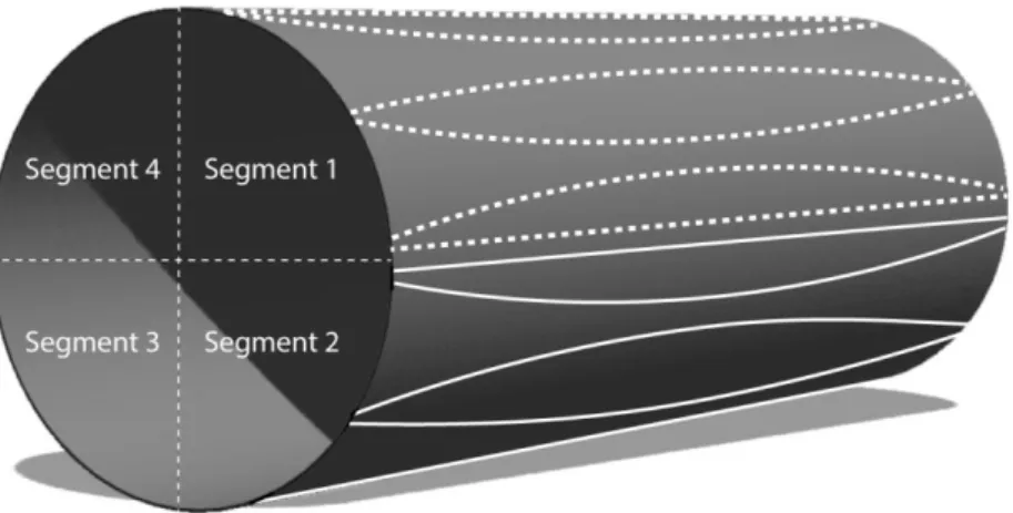
446
Figure 1: Schematic representation of a dynamically harmonized ICR cell. The cell is 447
divided into four segments representing each adjustable parameter: Segment 1 (in dashed 448
lines) is for shimming and gating 0°, segment 2 (in solid lines) for shimming and gating 449
90°, segment 3 for shimming and gating 180° and segment 4 for shimming and gating 270°. 450
451 452
22 453
Figure 2: a) Observation of the effects of the different factors on the even harmonic 454
magnitude for the screening step, b) Prediction plot between the predicted and observed 455
values of the second harmonic magnitude for the screening step, c) Observation of the 456
effects of the different factors on the second harmonic magnitude for the optimization step, 457
d) Prediction plot between the predicted and observed values of the second harmonic 458
magnitude for the optimization step. 459
460 461
23 462
Figure 3: LDI spectrum in positive mode of a tholins sample obtained after deploying the 463
cell parameter optimized with the DoE approach, revealing more than 50,000 peaks. The 464
inset visualized a close zoom between m/z 581.15 and m/z 581.40 illustrating the high 465
isobaric complexity. 466
467
Figure 4: (Top) Zoom on the tholins spectrum obtained after a manual optimization 468
(shimming) of the ICR cell parameters. (Bottom) Tholins spectrum obtained after applying 469
the parameters given by the DoE optimization. Red dots indicate species found after DoE 470
optimization and not detected after manual optimization. 471
24 473
Figure 5: Comparison of attributed peaks, global intensity, resolution and RMS between 474
the manually optimized spectrum and the DoE spectrum of a tholins sample. 475
476
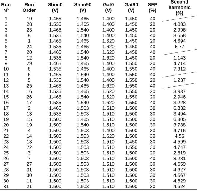
Table 1: Coded composite face design (CCF) design matrix for experimental
477
screening on NaTFA
478
Run N° Run Order Shi0 Shi90 Gat0 Gat90 SEP
1 10 -1 -1 -1 -1 1 2 28 1 -1 -1 -1 -1 3 23 -1 1 -1 -1 -1 4 9 1 1 -1 -1 1 5 1 -1 -1 1 -1 -1 6 24 1 -1 1 -1 1 7 20 -1 1 1 -1 1 8 12 1 1 1 -1 -1 9 29 -1 -1 -1 1 -1 10 8 1 -1 -1 1 1 11 6 -1 1 -1 1 1 12 5 1 1 -1 1 -1 13 25 -1 -1 1 1 1 14 16 1 -1 1 1 -1 15 26 -1 1 1 1 -1 16 17 1 1 1 1 1 17 2 -1 0 0 0 0 18 13 1 0 0 0 0 19 15 0 -1 0 0 0 20 19 0 1 0 0 0 21 4 0 0 -1 0 0 22 14 0 0 1 0 0 23 18 0 0 0 -1 0 24 22 0 0 0 1 0 25 3 0 0 0 0 -1 26 7 0 0 0 0 1 27 27 0 0 0 0 0 28 31 0 0 0 0 0 29 30 0 0 0 0 0 30 11 0 0 0 0 0 31 21 0 0 0 0 0
25 479
26
Table 2: Predicted values for each factor for the screening and optimization
481 step 482 483 484 485 486 487 488 489 490 491 492
Table 3. Comparison of the mass spectrometric response of the LDI tholins
493
spectra deploying manufacturer default values (before tuning), conventional
494
manual tuning (manual), and parameters given by the DoE optimization
495
method. p-values refers to the comparison between manual Tuning and the
496
DoE strategy. (p-value > 0.05 is considered as significant)
497
498
499
Screening step
Factor Intervals Predicted Value Factor contribution (%) Shim0 1.465 to 1.535 (V) 1.535V 15.4 Shim90 1.465 to 1.540 (V) 1.540V 33.3 Gat0 1.4 to 1.620 (V) 1.620V 12.6 Gat90 1.450 to 1.550 (V) 1.550V 10.7 Sweep 20 to 40 (%) 20% 28.0 Optimization step
Factor Intervals Predicted Value Factor contribution (%) Shim0 1.530 to 1.550 (V) 1.542V 53.1
Shim90 1.530 to 1.550 (V) 1.550V 43.4
Gat0 1.600 to 1.640 (V) 1.600V 1.9
Gat90 1.540 to 1.570 (V) 1.551V 1.7
DoE (Mean) Manual (Mean) p-value Fold Change
Attributed Peaks 1.76 10+04 1.55 10+04 9.69 10-05 1.13
Global Intensity 4.80 10+08 3.61 10+08 3.36 10-06 1.33
Resolution at m/z 400 1.44 10+06 1.35 10+06 1.24 10-07 1.07
27
Supplementary Information for
500
Optimization of ion trajectories in a dynamically harmonized
501
Fourier-Transform Ion Cyclotron Resonance cell using a Design of
502
Experiments strategy
503 504
Julien MAILLARD1,2, Justine FEREY2, Christopher P. Rüger2, Isabelle SCHMITZ-505
AFONSO2, Soumeya BEKRI3, Thomas GAUTIER1, Nathalie CARRASCO1, Carlos 506
AFONSO2 and Abdellah TEBANI2.3* 507
508
1LATMOS/IPSL, Université Versailles St Quentin, UPMC Université Paris 06, CNRS, 11 509
blvd d’Alembert, F-78280 Guyancourt, France
510
2 Université de Rouen, Laboratoire COBRA UMR 6014 & FR 3038, IRCOF, 1 Rue 511
Tesnière, 76821 Mont St Aignan Cedex, France 512
3 Department of Metabolic Biochemistry, Rouen University Hospital, Rouen, 76000, 513
France 514
This PDF file includes:
515
Tables S-1 to S-6 516
Captions:
517
Table S-1: Fractional Factorial design matrix with response values for the 518
screening step. 519
Table S-2: Fractional Factorial design matrix with response values for the 520
optimization step. 521
Table S-3: PLS model regression coefficients generated by the screening step. 522
Table S-4: ANOVA test results of the PLS model generated by the screening step. 523
Table S-5: PLS model regression coefficients generated by the optimization step. 524
Table S-6: ANOVA test results of the PLS model generated by the optimization 525
step. 526
28 527
528
Table S-1: Fractional Factorial design matrix with response values the screening step.
Run No Run Order Shim0 (V) Shim90 (V) Gat0 (V) Gat90 (V) SEP (%) Second harmonic (%) 1 10 1.465 1.465 1.400 1.450 40 2 28 1.535 1.465 1.400 1.450 20 4.083 3 23 1.465 1.540 1.400 1.450 20 2.996 4 9 1.535 1.540 1.400 1.450 40 3.558 5 1 1.465 1.465 1.620 1.450 20 4.694 6 24 1.535 1.465 1.620 1.450 40 6.77 7 20 1.465 1.540 1.620 1.450 40 8 12 1.535 1.540 1.620 1.450 20 1.143 9 29 1.465 1.465 1.400 1.550 20 4.714 10 8 1.535 1.465 1.400 1.550 40 7.312 11 6 1.465 1.540 1.400 1.550 40 12 5 1.535 1.540 1.400 1.550 20 1.237 13 25 1.465 1.465 1.620 1.550 40 14 16 1.535 1.465 1.620 1.550 20 3.937 15 26 1.465 1.540 1.620 1.550 20 2.946 16 17 1.535 1.540 1.620 1.550 40 3.228 17 2 1.465 1.503 1.510 1.500 30 6.332 18 13 1.535 1.503 1.510 1.500 30 3.494 19 15 1.500 1.465 1.510 1.500 30 6.305 20 19 1.500 1.540 1.510 1.500 30 3.788 21 4 1.500 1.503 1.400 1.500 30 4.716 22 14 1.500 1.503 1.620 1.500 30 4.56 23 18 1.500 1.503 1.510 1.450 30 4.599 24 22 1.500 1.503 1.510 1.550 30 4.747 25 3 1.500 1.503 1.510 1.500 20 2.819 26 7 1.500 1.503 1.510 1.500 40 8.281 27 27 1.500 1.503 1.510 1.500 30 4.659 28 31 1.500 1.503 1.510 1.500 30 4.627 29 30 1.500 1.503 1.510 1.500 30 4.567 30 11 1.500 1.503 1.510 1.500 30 4.629 31 21 1.500 1.503 1.510 1.500 30 4.624
29
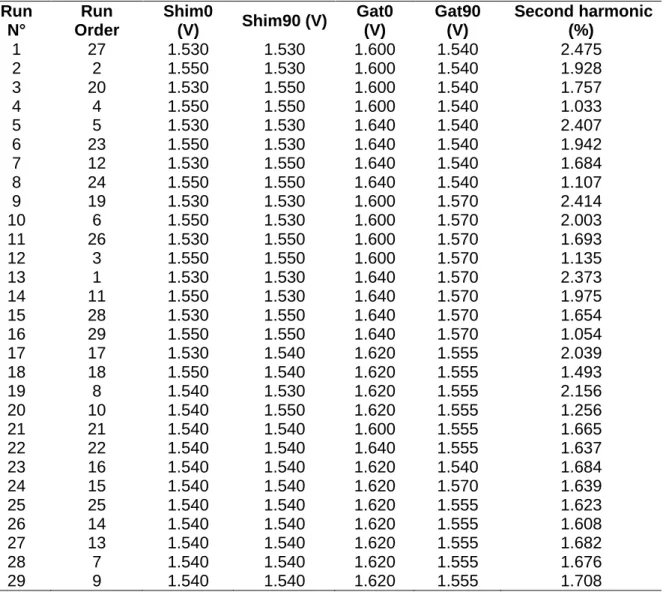
Table S-2: Fractional Factorial design matrix with response values for the optimization step. Run N° Run Order Shim0 (V) Shim90 (V) Gat0 (V) Gat90 (V) Second harmonic (%) 1 27 1.530 1.530 1.600 1.540 2.475 2 2 1.550 1.530 1.600 1.540 1.928 3 20 1.530 1.550 1.600 1.540 1.757 4 4 1.550 1.550 1.600 1.540 1.033 5 5 1.530 1.530 1.640 1.540 2.407 6 23 1.550 1.530 1.640 1.540 1.942 7 12 1.530 1.550 1.640 1.540 1.684 8 24 1.550 1.550 1.640 1.540 1.107 9 19 1.530 1.530 1.600 1.570 2.414 10 6 1.550 1.530 1.600 1.570 2.003 11 26 1.530 1.550 1.600 1.570 1.693 12 3 1.550 1.550 1.600 1.570 1.135 13 1 1.530 1.530 1.640 1.570 2.373 14 11 1.550 1.530 1.640 1.570 1.975 15 28 1.530 1.550 1.640 1.570 1.654 16 29 1.550 1.550 1.640 1.570 1.054 17 17 1.530 1.540 1.620 1.555 2.039 18 18 1.550 1.540 1.620 1.555 1.493 19 8 1.540 1.530 1.620 1.555 2.156 20 10 1.540 1.550 1.620 1.555 1.256 21 21 1.540 1.540 1.600 1.555 1.665 22 22 1.540 1.540 1.640 1.555 1.637 23 16 1.540 1.540 1.620 1.540 1.684 24 15 1.540 1.540 1.620 1.570 1.639 25 25 1.540 1.540 1.620 1.555 1.623 26 14 1.540 1.540 1.620 1.555 1.608 27 13 1.540 1.540 1.620 1.555 1.682 28 7 1.540 1.540 1.620 1.555 1.676 29 9 1.540 1.540 1.620 1.555 1.708 529
30
Table S-3: PLS model regression coefficients generated by the screening step.
Second harmonic Coeff. SC Std. Err. P Shim0 -0.08870 0.01303 0.00049 Shim90 -0.11241 0.01455 0.00025 Gat0 -0.00704 0.01455 0.64563 Gat90 0.00193 0.01455 0.89872 SEP 0.14123 0.01303 0.00004 Shi0*Shi0 -0.00072 0.01310 0.95773 Shi90*Shi90 0.00442 0.01369 0.75791 Gat0*Gat0 -0.01040 0.01368 0.47577 Gat90*Gat90 -0.00789 0.01368 0.58525 SEP*SEP 0.00569 0.01310 0.67912 Shi0*Shi90 -0.04575 0.01633 0.03106 Shi0*Gat0 -0.00388 0.01633 0.81987 Shi0*Gat90 -0.00052 0.01633 0.97560 Shi0*SEP -0.01725 0.01162 0.18826 Shi90*Gat0 -0.00212 0.01669 0.90321 Shi90*Gat90 -0.00107 0.01669 0.95099 Shi90*SEP 0.03057 0.01633 0.11029 Gat0*Gat90 0.00019 0.01668 0.99123 Gat0*SEP -0.00032 0.01633 0.98493 Gat90*SEP 0.00031 0.01633 0.98555 N = 27 Q2 = 0.628 DF = 6 R2 = 0.991 RSD = 0.03919 Comp. = 4 R2 adj. = 0.959 Confidence = 0.95 530
Table S-4: ANOVA test results of the PLS model generated by the screening step.
Second harmonic DF SS MS (variance) F p Total 27 11.0417 0.40895 Total corrected 26 0.972344 0.0373979 Regression 20 0.96313 0.0481565 31.3577 0 Residual 6 0.00921428 0.00153571 N = 27 Q2 = 0.628 Cond. no. = 12.05 DF = 6 R2 = 0.991 RSD = 0.039 19 Comp. = 4 R2 adj. = 0.959 531 532 533 534
31
Table S-5: PLS model regression coefficients generated by the optimization step. Second harmonic Coeff. SC Std. Err. P Constant 1,66208 0,0126069 4,58E-23 Shim0 -0,214759 0,0072904 5,37E-14 Shim90 -0,325479 0,00729039 1,69E-16 Gat0 -0,0120755 0,0072904 0,119882 Gat90 -0,00339587 0,0072904 0,648523 Shi0*Shi0 0,0608795 0,0154223 0,00145892 Shi90*Shi90 0,0117455 0,0154223 0,458943 Gat0*Gat0 -0,00371134 0,0154223 0,813317 Gat90*Gat90 0,0132228 0,0154223 0,405672 Shi0*Shi90 -0,0255319 0,00619991 0,00104456 Shi0*Gat0 0,00798444 0,0061999 0,218685 Shi0*Gat90 0,0138399 0,0061999 0,0424476 Shi90*Gat0 0,000118387 0,0061999 0,985034 Shi90*Gat90 -0,0022854 0,0061999 0,717926 Gat0*Gat90 -0,00542158 0,0061999 0,39662 N = 29 Q2 = 0,889 DF = 14 R2 = 0,995 RSD = 0,03858 Comp. = 5 R2 adj. = 0,991 Confidence = 0,95 535
Table S-6: ANOVA test results of the PLS model generated by the optimization step.
Second harmonic DF SS MS (variance) F p Total 29 92,3573 3,18473 Total corrected 28 4,41765 0,157773 Regression 14 4,39681 0,314058 211,033 0 Residual 14 0,0208347 0,00148819 N = 29 Q2 = 0,889 Cond. no. = 6,106 DF = 14 R2 = 0,995 RSD = 0,03858 Comp. = 5 R2 adj. = 0,991 536 537
32
Table S-7: Attribution of new peaks detected after the DoE optimization 538
539
Measured m/z
Molecular formula
Err. (ppm)
592.24866 C25H30N13O5 0.13 592.27374 C26H32N13O3^18O -0.04 592.28203 C27H35N10O5^13C -0.05 592.31836 C38H38N7 -0.06 592.32791 C19H41N14O7^15N -0.14 592.33949 C25H43N10O6^13C 0.03 592.34673 C19H43N14O7^13C -0.01 592.37013 C33H43N10^13C -0.11 592.37597 C26H47N10O5^13C -0.12 592.38314 C30H46N11O2 -0.17 592.39528 C35H47N8^13C -0.17 592.41238 C37H50N7 -0.11