Design and modeling of an active aeroelastic wing

(1)

Design and Modeling of an Active Aeroelastic Wing

Gregory W. Reich

Bachelor of Aerospace Engineering

Georgia Institute of Technology, Atlanta, Georgia (1992)

Submitted to the Department of Aeronautics and Astronautics in partial fulfillment of the requirements for the degree of

MASTER OF SCIENCE in AERONAUTICS AND ASTRONAUTICS

at the

Massachusetts Institute of Technology

February 1994

The author hereby grants to MIT permission to reproduce and to distribute publicly copies of this thesis document in whole or in part.

Signature of Author

Department of Ae rna tics and Astronautics January 21, 1994

Certified by

Professor Edward F. Cr(wley MacVicar Faculty Fellow, Professor of Aeronautics and Astronaitcs

Thesis Supervisor

Accepted by A S

FMAbl 7 sHsS NSTITUTE

FEB 17 1994

I I

ifrofessor Harold Y. Wachman Chairman, Department Graduate Committee

(2)

Design and Modeling of an Active Aeroelastic Wing

Gregory W. Reich

Submitted to the Department of Aeronautics and Astronautics in partial fulfillment of the requirements of the degree of

IASTER OF SCIENCE in AERONAUTICS AND ASTRONAUTICS

Abstract

The design modeling, and benchtop testing of a wing with strain and conventional flap actuation for vibration and flutter suppression is presented. The model hardware is described in terms of the design requirements. The design of an integrated safety system for flutter suppression is detailed. Model components are dynamically tested using an aluminum test article similar to the final design. Ground vibration testing and identification methods are developed using the testbench, and compared to finite element models to validate the analytical modeling. The actual model is tested using an electrodynamic shaker and accelerometers at a grid of points over the structure, and the model is identified using a frequency response-based method. The finite element model of the wing is validated via qualitative frequency response and node line contour comparisons with the identified model, and via quantitative measures of the modal frequencies and the Modal Acceptance Criterion. Finally, the validated analytical model is used for predictions of the aeroelastic behavior of the wing.

Thesis Supervisor: Dr. Edward F. Crawley

(3)

Acknowledgments

First off, I would like to thank my advisor, Ed Crawley, for his

knowledge, help, and understanding in my helter-skelter, full-blast approach to getting a degree. There's got to be a better way to do it, but thanks for letting me do it my own way. I would like to thank Tienie van Schoor for his day-to-day help, support, and friendship. If I could give co-advisement billing to the thesis, the second, equally as important as the first, would be yours.

I would also like to acknowledge all of the members of the wing gang. It truly has been a team effort, you all deserve to be recognized. The wing gang is: Paul, Chris, Mark, Dina, Tienie, Charrissa, Kim, and UROPers Alfredo, Brian, J. P., John, and Enrique.

Grad school would not be the experience that it is without other students to share it with. To everyone in SERC, a big thank you for the times we have shared. Thanks go to Yool for putting up with me for the last year and a half (!). To Charrissa, thanks for the help and understanding, both technically and socially. You are a great friend and a wonderful person. I would also like to thank all of my other friends in the lab, especially Roger, Brett, Becky, Simon, Mark, Carl, Dina, and Kim, for providing me the excuse to do something besides work. Included in this boat are all of my friends outside the lab, especially Russ, and the rest of MIT grad soccer.

A big thanks must also go to my family. Unfailing support can sometimes be taken for granted, but this is the one time that I can publicly thank all of you for all that you have done. I cannot say enough about how much your support and love means to me. To Mr. and Mrs. L. W. Reich, and Mr. and Mrs. C. A. Shannon, my grandparents and the people to whom this thesis is dedicated, thank you especially for the long distance support.

This thesis is also dedicated to Christy, without whom I would not be the person I am today. Your thoughtfulness, dedication, and commitment to me have meant more than you know, or I can express properly. Wherever we may be, together or apart, you must know how much I appreciate you. I hope that I can have the chance to do the same for you someday.

Financial support was provided by the U. S. Air Force, in the form of a Palace Knight student sponsorship.

(4)

List of Figures

Figure Figure Figure Figure 2.1: 2.2: 2.3: 2.4: Figure 2.5: Figure 2.6: Figure 2.7: Figure 2.8: Figure Figure Figure Figure Figure Figure Figure Figure Figure 2.9: 2.10 2.11 2.12 3.1: 3.2: 4.1: 4.2: 4.3: Figure 4.4: Figure 4.5:

Top view of the active wing wind tunnel model ... 15

Spar dimensions and layout ... ... . 16

Details of spar cross-sections ... ... . 17

Cross-section and top view of root attachment, including bolt pattern ... 18

Wind tunnel support structure and mounting assembly interface ... ... 18

Piezoceramic package placement on wing... 19

Top view and cross-section detail of one piezoceramic actuator package ... ... 20

Detail of spar cross-section with piezos and applied signal (not to scale) ... 21

Flap drive system ... ... ... 22

Cross-section of the flap... ... 23

Location of shell attachments to spar and flutter stopper ... 24

Detail of a "typical" shell section... 25

Mass deployment schematic ... 30

Cross-section and top view (assembly drawing) of the flutter stopper ... 32

Experim ental test setup ... ... 38

Sensor and actuator locations on the FEM grid... 40

Frequency response functions for measured data and identified system of the testbench at location 27 ... 42

Fixed boundary node locations on the finite element mesh, viewed from above and behind the trailing edge tip ... 44

Element group regions and composition of the finite element mesh for the testbench ... 45

(7)

Figure 4.6: Bending degrees of freedom for beam elements ... 46 Figure 4.7: Schematic of an extra connecting element from the drive

shaft to a bearing mount ... ... .. 46 Figure 4.8: Transfer functions from the finite element model of the

testbench, location 27 ... ... 48 Figure 4.9: Modal contour plots on a cartesian grid for the testbench

from experimental and finite element models: (a),

undeployed configuration; (b), deployed configuration ... 49 Figure 4.10(a): Transfer functions from location 4 to location 30 from

experimental and finite element models for the testbench (undeployed model) ... ... 51 Figure 4.10(b): Transfer functions from location 4 to location 30 from

experimental and finite element models for the testbench (deployed m odel) ... ... ... 52 Figure 4.11: Element group regions and compositions for the

composite spar finite element model ... 56 Figure 4.12: Experimental test setup for the composite spar... 57 Figure 4.13: Modal contour plots on a cartesian grid for the composite

spar without the shell from experimental and finite element models (a), undeployed configuration modes 2 and 3; (b), deployed configuration modes 2 and 3; (c), undeployed configuration mode 4; (d), deployed

configuration mode 4... ... 60 Figure 4.14(a): Transfer functions from location 40 to location 30 from

experimental and finite element models for the wing

without the shell (undeployed model) ... 61 Figure 4.14(b): Transfer functions from location 40 to location 30 from

without the shell (deployed model) ... 62 Figure 4.15(a): Transfer functions from location 25 to location 30 from

with the shell (undeployed model) ... 65 Figure 4.15(b): Transfer functions from location 25 to location 30 from

(8)

Figure 4.16: Figure 4.17: Figure 4A.1: Figure 4A.2: Figure 4B.1: Figure 4B.2: Figure 4C.1:

Modal contour plots on a cartesian grid for the composite spar with the shell from experimental and finite element models; (a), undeployed configuration modes 2 and 3; (b), deployed configuration modes 2 and 3; (c), undeployed

configuration mode 4; (d), deployed configuration mode 4... 68 Mode 4 node line contour plots of the undeployed flutter

stopper experimental and finite element models for the composite spar with the shell; (a), original models; (b), original experimental model, FE model with artificial

zero-order structural sag... ... 69 Undeployed modeshapes for the testbench for

experimental and finite element models (trailing edge

out, root on the left)... ... 71 Deployed modeshapes for the testbench for experimental

and finite element models (trailing edge out, root on the

left) ... 72 Undeployed modeshapes for the spar without the shell for experimental and finite element models (trailing edge

out, root on the left) ... ... ... 73 Deployed modeshapes for the spar without the shell for

out, root on the left)... ... ... 74 Undeployed modeshapes for the spar with the shell for

out, root on the left) ... ... ... 75 Figure 4C.2: Deployed modeshapes for the spar with the shell for

out, root on the left) ... ... ... 76 Figure B.1: Natural frequency versus airspeed for the first four modes

of the flutter stopper undeployed system... 87 Figure B.2: Damping ratio versus airspeed for the first four modes of

the flutter stopper undeployed system ... 87 Figure B.3: Natural frequency versus airspeed for the first four modes

of the flutter stopper deployed system ... 88 Figure B.4: Damping ratio versus airspeed for the first four modes of

(9)

List of Tables

Table 3.1: Functional requirements and design goals for the flutter

stopper ... 29 Table 3.2: Dimensions and properties of the flutter stopper ... 35 Table 4.1:

Table 4.2:

Table 4.3:

Table 4.4:

Comparison of the testbench experimental and finite element in-vacuo natural frequencies for the undeployed

and deployed configurations (in Hz)... 53 MAC values for the testbench for the undeployed and

deployed configurations ... ... 54 Comparison of composite spar experimental and finite

element in-vacuo natural frequencies for the undeployed and deployed configurations without the aerodynamic shell

(in H z) ... 58 MAC values for the composite spar in the undeployed and

deployed configurations without the aerodynamic shell... 59 Table 4.5: Weight breakdown of major components of the wing model... 63 Table 4.6:

Table 4.7:

Table B.1:

Table B.2:

Comparison of experimental and finite element in-vacuo natural frequencies for the composite spar with the

aerodynam ic shell (in Hz) ... 64 MAC values for the composite spar with the aerodynamic

shell for undeployed and deployed cases... 66 Frequency and damping ratios of the undeployed flutter

stopper model at selected airspeeds from analytical flutter

predictions ... 86 Frequency and damping ratios of the deployed flutter

stopper model at selected airspeeds from analytical flutter

(10)

Introduction

Chapter 1

Aeroelastic wing vibration is a major concern to the modern aircraft engineer. Vibrations from gust loading or other sources affect the fatigue life and integrity of the aircraft structure. Gust loading also affects the ride comfort of the passenger. Instabilities such as flutter of wing or stores affects the maximum flight speed and endangers the integrity of the craft. Controlling gusts and other random vibrations helps reduce fatigue and ride comfort, while flutter suppression can increase the flight envelope and improve the safety of the structure.

Aeroelastic control of wing vibrations and instabilities is achieved by both passive and active means. Passive methods include structural tailoring of the wing, such as adjusting geometric sweep, or tailoring of the composite laminates used in the wing's construction. Active methods involve using the control surfaces of the wing as actuators. Recent studies have combined both of these methods.

A newer approach to aeroelastic control uses both active and passive methods, but is fundamentally different from other existing methods. Structural tailoring is used as it was before, shaping the bend/twist coupled

(11)

response of the wing that is desired. However, instead of control surfaces, strain actuators apply the controlling forces directly to the wing structure. In this way, many of the delays which hamper the conventional methods are circumvented: there are no hydraulics necessary to actuate the control surfaces, and there are no aerodynamic lags associated with the application of the control forces and moments.

Preliminary studies on aeroelastic tailoring investigated bend/twist coupling on cantilevered composite plates in a wind tunnel to verify analytically predicted flutter and divergence speeds [Hollowell and Dugundji, 1984]. Subsequent studies included geometric sweep in the models [Landsberger and Dugundji, 1985]. Active control techniques were being developed concurrently which were applied to flutter suppression experiments. Turner [1975] showed analytically that flutter suppression could be done on a high aspect ratio wing using an aileron as the actuator. In an international effort, wing-store flutter suppression was investigated on a 30% scale half span model of the YF-17 using leading and trailing edge control surfaces [Hwang, et al, 1980]. Free flight tests with a drone model were conducted to validate various control methods of flutter suppression [Newsom, Pototsky, and Abel, 1985]. Multiple leading and trailing edge surfaces were combined on a scale model of an "F-16 derivative planform" wing [Pendleton, Lee, and Wasserman, 1992]. Recently, aeroelastic tailoring was combined with control surface actuation in a series of tests on the Active Flexible Wing (AFW) program [Perry, et al, 1990]. The AFW model is a rigid fuselage, flexible wing scale model of an advanced tailless fighter. The wings are constructed of bend/twist coupled composite plates, and each wing includes two leading edge and two trailing edge control surfaces.

(12)

This conventional method of aeroelastic control has been used in the majority of flutter and vibration suppression experiments. This is primarily due to the existence of high-authority control surfaces on the wings in use. However, because these surfaces are not designed for this purpose, they are not necessarily the optimal actuators to use. The complete actuation mechanism includes significant aerodynamic and hydraulic lags because these actuators are typically hydraulic, and must generate aerodynamic forces to control the wing. In addition, ailerons typically operate over a limited bandwidth, which does not necessarily include the aeroelastic modes of interest.

Strain actuation is the alternative to flap actuation. Early studies in the use of strain actuation focused on characterizing the behavior of a certain type of strain actuators: piezoelectric, or piezoceramic, actuators [Crawley and Lazarus, 1991]. Analytical studies on the static aeroelastic behavior of wing models have been conducted [Ehlers and Weisshaar, 1990]. A simple two degree of freedom wind tunnel model demonstrated strain actuated

flutter suppression [Heeg, 1992]. A more sophisticated experiment,

demonstrating vibration and flutter suppression using multivariable control on a plate-like lifting surface with piezoelectric actuators, was successfully completed [Lazarus and Crawley, 1992]. This latter work forms the basis for the current study, which takes the technology developed by Lazarus and Crawley, and applies it to a larger, more wing-like model. The design and development for this program is presented by Lin and Crawley [1993].

The objective, then, of this research study is to investigate the effectiveness of a strain-actuated aeroelastic control system, and to compare its performance in gust alleviation and flutter suppression against a control-surface actuated control system on a wing flutter model. In this document,

(13)

the design and manufacture of the wing model, and issues in the development of the mathematical and experimental models required for verification, analysis and prediction of the structural behavior of the wing model are studied.

The finite element model is initially developed as an analysis tool to make intermediate decisions during the design process. Then, the design is constructed and experimental tests are run to identify the model. The finite element model is compared to the identified model to validate the analysis, and the analysis is iterated until the model errors fall within an acceptable bound.

The first section of this study explains the model hardware. Chapter 2 contains a description of the active wing flutter model in terms of the design requirements previously determined [Lin and Crawley, 1993]. All components are discussed in detail, and emphasis is placed on the method of attachment of one component to another. The description continues in chapter 3, where the design of an integrated safety system for flutter suppression is presented.

The second section of the thesis investigates the development and implementation of analytical and experimental modeling techniques for the program. The first part of chapter 4 describes the creation of a testbench model to replicate the "flight" hardware. The testbench will also used to develop experimental procedures for the identification of the wing model. These experimental models will then be compared to mathematical models as a validation of the finite element analyses. The second part of chapter 4 contains the application of these modeling techniques, both experimental and theoretical, to the wing model. The two models will be compared, and analysis on the similarities and differences presented.

(14)

Active Flutter Model Description

Chapter 2 2.0 Introduction

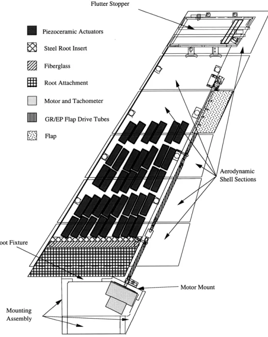
In order that the analysis and discussion that follows can be taken in context, it is desirable to first describe the physical set-up and hardware. An overall view of the active flutter model is pictured in Figure 2.1, which shows all of the major assemblies. The components of the active wing are built up on and around the spar, and include the piezoceramic actuators, the root attachment, mounting bracket and motor mount, the flap drive, the flutter stopper, and the aerodynamic shell. The design requirements for the project are covered in detail by Lin and Crawley [1993], and thus only the major requirements that affect each component will be discussed. This chapter contains a detailed description of each sub-component of the experimental hardware.

2.1 Wing Spar and Root Attachment

The spar is the load-bearing structure of the wing, and the foundation for the rest of the model. Its shape was required to be

(15)

Flutter Stopper

Piezoceramic Actuators Steel Root Insert Fiberglass Root Attachment

D

Motor and Tachometer

Ml GR/EP Flap Drive Tubes

jFlap Aerodynamic Shell Sections Root Fixture Motor Mount Mounting Assembly

Figure 2.1: Top view of the active wing wind tunnel model

geometrically representative of aircraft wings in which bending/torsion flutter is critical, in order to compare its performance with real aircraft.

Other design requirements included: the spar must have a flutter

mechanism consisting of a coalescence of the first two modes; it must

flutter well below transonic conditions; it must have modest structural

(16)

18.00

41.57

B

31.530

Steel Root Insert

A Fiberglass & Insert Cover

Wing quarter chord

12.00

Aluminum Inserts

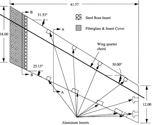
Figure 2.2: Spar dimensions and layout

thickness without necessitating the complications of a monocoque wing structure; and it must enable independent control of the first two modes by strain actuation.

To meet these requirements, a spar was designed and built from 2 IM7G/3501-6 graphite-epoxy plates of [20'2/01], laminate. Each plate, 0.032" thick, is bonded to an aluminum honeycomb core 0.177" thick. The lay-up angles are referenced to the wing quarter-chord, which is swept 300 (see figure 2.2). This unsymmetric lay-up, combined with wing sweep, produces washout at the tip, as well as bend/twist coupling, which is instrumental in control of the torsional mode of vibration [Crawley and Lazarus, 1991]. The honeycomb core provides 2% structural thickness and allows enhanced bend/twist coupling.

I

(17)

--Graphite/Epoxy (0.032") 0.177 Section A-A Aluminum Honeycomb

Section B-B

4

Fiberglass (.( A;AxV.xx. 0, Pf9 0.,9. . 9 0.241" )20") 0.177 0.281" Steel Insert Graphite/Epoxy (0.032")

Figure 2.3: Details of spar cross-sections

Figure 2.2 shows the physical dimensions of the spar (see Appendix A for physical properties of the materials). At the root, the honeycomb core is replaced with a 5.6" wide mild steel insert, and 4.75" wide fiberglass strips are added on top of the graphite-epoxy. The fiberglass strips consist of 3 layers of E-glass fabric, [0/90] lay-up, which increases the spar thickness by a total of 0.040". Cross sections A-A and B-B of Figure 2.2 are shown in more detail in Figure 2.3. Here the relative thicknesses of each material can be seen. The steel insert is designed to help relieve the high stress concentrations that exist at the root, and the fiberglass layers are designed to protect the graphite-epoxy and insure a smooth joint between the spar root and root attachment. The hole pattern for the root attachment bolts is also visible in Figure 2.2, as well as the eleven solid aluminum inserts replacing the honeycomb around the periphery of the spar. These allow for other attachments to the spar, such as the flap drive bearing mounts (Fig. 2.6), the shell (Fig. 2.7), and the flutter stopper (Fig. 3.2). The two inserts for flutter stopper mounts on the wingtip have tabs to prevent

(18)

Section C-C

G---

---Trailing

/e--

-

O

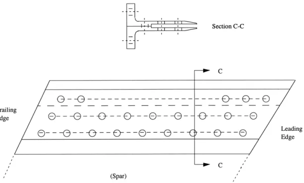
--- C -- O--- -C (Spar)

Figure 2.4: Cross-section and top view of root attachment, including bolt pattern

Figure 2.4 shows two views of the root attachment. The spar slides into the slot, and is secured by eighteen 1/2" diameter steel through bolts. The root attachment enforces a near cantilever boundary condition by transferring loads to the root fixture, and from there to the rigid wind tunnel support, as shown in Figure 2.5. The mounting assembly, all

Root Fixture

LaRC Rigid Support _{Mounting Assembly}

Motor and Tachometer

Tunnel Wall

Motor Mount

Figure 2.5: Wind tunnel support structure and mounting assembly interface

S Ed ding :e I I I I I _I _I

(19)

..

_I_-IY- -~ -gI~~--Y

machined aluminum plates, serves as an interface between the spar and the LaRC rigid support, which extends several feet out from the wind tunnel wall. To isolate the model aerodynamically from the mounting structure, a splitter plate (not shown) was used. This 4' x 8' aluminum panel was mounted vertically at the root fixture to separate the wing assembly from the mounting assembly.

2.2 Piezoceramic Actuators

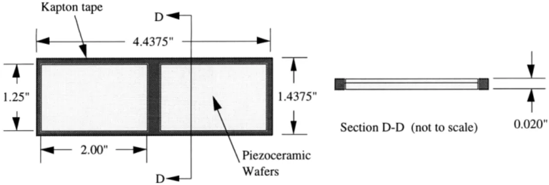
Strain actuation is carried out by the 72 piezoceramic actuator packages mounted on the top and bottom of the spar, pictured from above in Figure 2.6. The actuators covered 63% of the region between the 13% and 66% span locations. This coverage is approximately between the root attachment and the flap. Figure 2.7 shows a single package, which consists of 4 G-1195 piezoceramic wafers, two wide and two thick. The packages were made by imbedding the wafer stacks in kapton tape, and covering with a layer of polyurethane.

The amount (thickness) of wafers to be used was determined in a series of trade studies done by Lin and Crawley [1993] which indicated that

Piezoceramic actuator region

Steel Insert

(20)

Kapton tape

1.25" 1.4375"

_ _ Section D-D (not to scale) 0.020"

2.00" _Piezoceramic

D -Wafers

Figure 2.7: Top view and cross-section detail of one piezoceramic actuator package

while there is increasing authority on the bending mode as actuator thickness increases, there is an optimum thickness for torsional control. Because simple piezoceramics are elastically and piezoelectrically isotropic, they cannot provide shear strain, and thus do not have any authority over torsional motion. With an orthotropic plate, such as the spar, torsional control is possible because of the bend/twist coupling produced by the non-symmetric lay-up of the graphite-epoxy [Lazarus and Crawley, 1989]. As the actuator thickness is increased, however, the effects of the elastically isotropic actuation material begin to dominate the effects of the orthotropic plate, reducing the bend/twist coupling. The optimum thickness in this case was found to be 0.020".

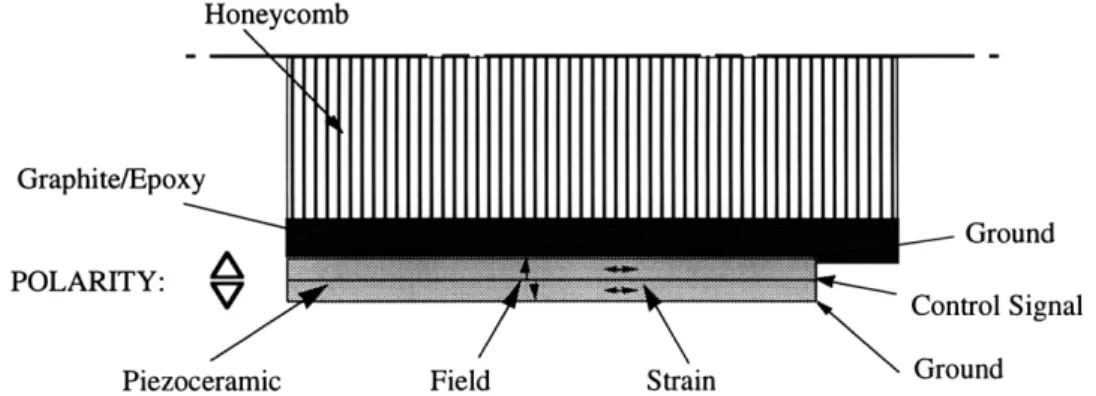
Strain actuation is applied by poling packages on opposite sides of the spar in opposite directions. The resulting strain is realized as a bending moment on the spar. The modal forcing is then controlled by arranging the actuator packages into fifteen blocks. These blocks are then arranged into actuation groups for control of two modes: one bending and one torsion. For bending, all of the blocks are actuated in the same direction. For torsion, the blocks are divided into two regions, roughly span-wise, and are actuated in opposing directions from each other. The grouping is ordered such that

(21)

Graphite/Epoxy

Ground POLARITY: ... ...

V . Control Signal

Piezoceramic Field Strain Ground

Figure 2.8: Detail of spar cross-section with piezos and applied signal (not to scale)

the two opposing regions of strain actuation are on opposite sides of the zero-curvature line for the torsion mode. Figure 2.8 shows the lower half of the spar cross-section with packages, and how the control signal is applied between layers of wafer, so that both the spar and the exposed surface are grounded. Each block of packages, consisting of four to six packages, is powered by one power amplifier, with a maximum of ±200 volts, which is roughly 2/3 of the coercive field strength of the piezoelectric material.

2.3 Flap Drive System

The flap drive system design was driven by the large size of the electric torque motor necessary to drive the flap. The impossibility of mounting the motor just inboard of the flap dictated that the motor be

placed outside of the wing in the mounting assembly, and connected to the

flap by a long drive shaft. The shaft would have to be sectioned and joined

with universal joints or other flexible members, due to the significant

bending of the spar under operational loads, to allow for clearance within

the aerodynamic shell. The drive shaft was also required to be extremely stiff in torsion to minimize the windup, and consequently maintain a high

(22)

level of flap motor authority over the actuation range. A sensor for measuring the flap angle would also have to be included in the design, and a local flap servo built to allow control of the flap angle from commanded inputs.

The drive system that developed is shown in Fig 2.9. The design centers around 3 hollow AS4/3501-6 graphite-epoxy shafts, each with a

[±450] lay-up repeated for maximum torsional strength. Zero-backlash steel

universal joints from Sterling Instruments are used between shafts to allow the flap to operate when the wing underwent large deflections. A GTC telescoping ball spline allows for axial play, and the drive is attached to the spar at three locations with mounts which hold miniature ball bearings. The whole drive system has ±0.150 windup at nominal operational torque levels due to aerodynamic loading on the flap.

The PMI U12M4HA pancake style torque motor and PMI U6T

Displacement Sensor Target and Mount

(23)

tachometer are mounted to the motor mount, which is angled to match the trailing edge sweep angle (see Figure 2.5). The motor mount is part of the mounting bracket assembly. Hard stops are added to limit the rotation of the motor to ±60. This protects the flap drive from over-rotation and the starting transient which the motor undergoes.

This system drives a flap that is 20% in both span and chord, and is located between the 60% and 80% span locations. The only requirement on the flap drive system was that the flap have enough chordwise stiffness to assume chordwise rigidity in the model. The flap is made from MXB-7251/181 fiberglass fabric of [0/45]s laminate, with a wall thickness of 0.040", and is mass balanced to decrease the complexity of the controller. The flap is bolted directly to the shaft (see Figure 2.10). Flap position is measured with a Kaman KD-2310-2UB inductive non-contact displacement sensor which targets an eccentric cam, whose relative location is pictured in Figure 2.9. The cam's slanted face moves perpendicularly with respect to

the sensor when the shaft rotates. The ±50 of flap angle is translated into a

0.080" travel of the cam face. Hard stops on the cam prevent it from over-rotating and destroying the sensor.

Mass Balance Weights

3.713"

Graphite Epoxy Tube

Figure 2.10: Cross-section of the flap

(24)

2.4 Aerodynamic Shell

In order for the model to be tested with a proper aerodynamic loading, a light-weight fiberglass shell was designed to cover the model and "shape" the aerodynamics. The requirements for the shell were defined as: the wing geometry should be representative of aircraft in which bending/torsion flutter is critical; the airfoil shape should not provide any lift at zero angle of attack; and the shell should not add appreciable stiffness to the spar. Adding stiffness would alter the structural dynamics and diminish the control authority of the actuators.

A sectioned fiberglass shell, made of MXB-7251/181 fabric in a

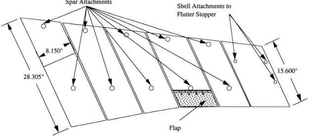
[0/45/0], laminate, was designed to provide these qualities. The 0.060" thick shell is shaped like a NACA 66-012 airfoil, divided into 5 spanwise sections, and fixed to the spar in only two locations per section (see Fig. 2.11). The shell completely envelops the spar and attached components. Its removable section design allows easy access to internal hardware. Each shell was designed as two half shells, bolted together through the spar at the leading

Spar Attachments

Figure 2.11: Location of shell attachments to spar and flutter stopper

(25)

and trailing edges. Figure 2.12 shows a detail of an attachment point on a typical shell section. The shell over the wingtip, which covers the flutter stopper, is attached in a slightly different manner.

The inserts are made from an epoxy that was bonded to the inner surface of the fiberglass after curing. This epoxy is hard enough to hold a tap, so inserts threaded on both inner and outer surfaces are bonded to the epoxy. These hold the bolts which pass through the spar and attach the two sides of the section. At the leading edge, the top half is made with a lip that overlaps the bottom half, so that the halves cannot separate during testing, allowing airflow through the shell. A filler is used at the leading and trailing edges, at the front for greater strength, and at the back for a good mating surface between top and bottom halves. Because a 0.30" chordwise gap remains between shell sections for clearance when the spar bends, foam is inserted between sections so that no air can flow under the shell.

foam sections encased in glass

inserts

spar

Overlapping lip on front edge No foam in this region Figure 2.12: Detail of a "typical" shell section

(26)

2.5 Flutter Stopper

In order to test the flexible flutter model in the wind tunnel, provisions for both the model's and the tunnel's safety are taken. Tunnel shut down is not an acceptable approach because the response time of the tunnel is much slower than necessary. Some other mechanism is required that can respond in the time interval of one or two vibration cycles. A mechanism that quickly changes the wing's aeroelastic properties at any given flight speed was designed and built. The system includes several sensors to detect the onset of flutter, which then trigger the firing mechanism. The system is the subject of the next chapter, which describes in detail the design and testing of an integrated flutter suppression system.

(27)

Integrated Flutter Suppression

System

Chapter 3 3.0 Introduction

As discussed briefly at the end of the last chapter, the wing design includes a safety system which aeroelastically stabilizes the model after the onset of flutter. The change in aeroelastic properties of the wing is accomplished by shifting the wing chordwise CG location, which causes a significant change in the stability of the wing at a given tunnel velocity. The CG shift is achieved by sliding a large mass forward along the tip of the wing. The flutter speed of the wing with the mass in the "undeployed" position is considered the nominal flutter speed of the system. Approximately 30% above this speed is the "deployed" flutter speed, where the mass is located in the forward, or deployed, position. This is the highest speed at which the wing can be safely tested, since the wing is aeroelastically unstable for either configuration at speeds above this point. This chapter discusses the design of the internal, integrated tip mass flutter stopper, both in terms of its functional requirements and the resulting design.

(28)

Flutter stopper systems are not an innovation in aeroelastic wind tunnel projects. As evidenced by the wide variation in types of flutter suppression devices, there are many different mechanisms of preventing or suppressing instabilities, and therefore the potential destruction of the model. Some simple designs physically restrained the model using stops or other dampers [Ricketts and Doggett, 1980]. More complicated systems encompassed the use of a wingtip or underwing store, designed to decouple the dynamics during flutter from the rest of the wing [Noll, et al, 1989]. Ejectable ballast have also been used to change the aeroelastic properties, although this is not optimal for the wind tunnel setting [Newsom, Pototzky, Abel, 1985]. The current design is based on a system used on the YF-17 flutter model program [Hwang, et al, 1980], which housed a sliding mass inside an AIM-7S wingtip store. However, as will be emphasized below, a store could not be used for this experiment, and the sliding mass was made internal to the wing cross-section.

3.0.1 Design Goals and Functional Requirements

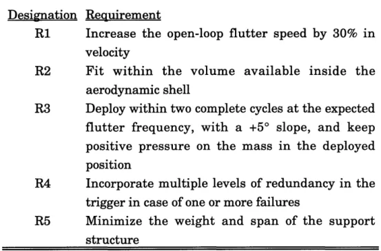
The set of specifications that any design must meet is referred to as the functional requirements [Suh, 1990], which can represent performance goals, constraints, regulatory, or safety requirements. There are five functional requirements listed in Table 3.1 which were to be met in order to achieve the design objective. Several of these were not absolute requirements, and were not posed as such. Rather, they were guidelines to steer the design during its development.

(29)

Table 3.1: Functional requirements and design goals for the flutter stopper Designation R1 R2 R3 R4 R5 Requirement

Increase the open-loop flutter speed by 30% in velocity

Fit within the volume available inside the aerodynamic shell

Deploy within two complete cycles at the expected

flutter frequency, with a +50 slope, and keep

positive pressure on the mass in the deployed position

Incorporate multiple levels of redundancy in the trigger in case of one or more failures

Minimize the weight and span of the support structure

3.1 Flutter Stopper Hardware

As a first step in the design, it was necessary to determine how much

mass was needed to meet requirement one of Table 3.1. This was

accomplished in a trade study done by Lin and Crawley [1993]. They

investigated some of the design parameters (physical properties) which could be varied, including size, weight, and CG location, and the effects that these had on the flutter speed of the wing in the deployed versus undeployed configuration. The analysis was done using a five mode Rayleigh-Ritz structural model of a multi-layered composite plate using unsteady, swept two-d strip theory aerodynamics with a one pole approximation of Theodorsen's function. This code was adapted from an earlier work by Lazarus and Crawley [1992]. The results of the study showed that a 1.5 kg

(30)

(3.3 lb.) mass, shifted from "slightly aft of the midchord" to the leading edge at the wingtip, would result in an increase of 30% in flutter speed.

Once the amount of mass needed was determined, completion of the design required refinement and compromise necessary to meet the remaining requirements. For example, in reality it was not possible to put the mass CG at the leading edge, since this would have caused the assembly to extend in front of the leading edge. This would have violated the second requirement (R2), which was to fit the entire structure inside the shell. The effects of this requirement are felt throughout the design.

Due to the rigorous volume constraints imposed by R2 and R5, a tungsten alloy was chosen as the material for the translating mass. This alloy (pure tungsten is more dense, but nickel and copper are added to improve machinability) is 50% heavier than lead, at approximately 0.6 lb/in.3. Many design iterations were performed varying the cross-sectional shape, width, and CG locations of the mass in an attempt to minimize the size and still meet all of the requirements.

The schematic problem of deployment is pictured in Figure 3.1. The initial and final locations xi and xf were chosen to be aft of the mid-chord, and as close as possible to the leading edge.. The spring size and strength were

-Xi

(31)

chosen by solving the dynamic spring-mass problem to satisfy the deployment requirement (R3). Because of the predicted torsional motion of the wingtip during flutter, the deployment was chosen to be up a constant 50 slope (angle of attack). This did not reflect the physical motion that the system would undergo, but simply increased the strength of the springs to meet the requirement. For a given deployment time, in this case two cycles at 8 Hz, or 0.25 seconds, the spring constant and spring length were inter-related. The longer the spring, the softer it could be. Of course the spring must also satisfy the geometrical constraints imposed by the spring's fully compressed solid length and inner and outer diameters. The springs were also chosen to meet the requirement that their compression length be longer than the travel distance, so that even in the deployed configuration the springs would be imparting a forward force on the mass. In order to provide redundancy in forward retention once deployed, a spring latch was added just behind the deployed mass location. Rubber bumpers were affixed to the front of the mass to cushion the collision with the leading edge frame.

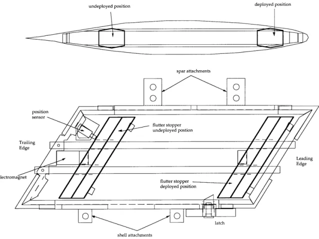
Figure 3.2 shows both top and cross-section views of the completed flutter stopper. The entire assembly fits inside the NACA 66-012 airfoil shape with chord equal to 15.6 inches, which is the chord at the tip of the shell. Both frame and mass are swept 31.90, which is the sweep of the leading edge of the shell. The mass is tapered on its forward and rearward facing sides to maximize the distance between fore and aft positions. Both inboard and outboard frames are similarly tapered, since these must extend further than the tungsten in both directions. The frame is made from 1/4" to 1/2" thick aluminum beams, designed for maximum stiffness with minimum weight (R5). For this reason they are channeled wherever possible, and

(32)

spar attachments

shell attachments

Figure 3.2: Cross-section and top view (assembly drawing) of the flutter stopper

The mass slides on two 3/8" diameter hardened steel rods. Two runners are used, as opposed to a single runner, to cut down on the possibility of rattle occurring. The rods are pinned into the trailing edge frame, and are held in alignment at the leading edge by precision-machined through holes. Their size and strength were chosen so that the bending frequency of the rods with the mass in the middle, the worst case scenario, was greater than 30 Hz. The flutter stopper is attached to the spar with brackets at the two inserts on the wingtip, located at approximately the 30% and 60% chord locations. These aluminum brackets slide over the spar, and are bolted through the aluminum inserts. The aerodynamic shell is attached at three locations: two aluminum outboard blocks, and at the 30% chord spar

(33)

attachment. The outboard blocks were designed to mimic the spar where the shell bolts through it, and the shell is fastened in the same manner as at further inboard locations over the spar. It was determined that this three-point attachment method is acceptable, since there was predicted to be little deflection, if any, of the flutter stopper relative to the wingtip.

The safety electronics of the flutter stopper were designed to monitor sensors for signs of impending flutter, deploy the tungsten mass, and shut

down all critical activities during deployment. In the undeployed

configuration an electromagnet holds the mass via an iron target on the trailing edge of the tungsten. The mass is deployed when the safety circuit shuts off power to the magnet. The circuit monitors different sensors on the wing, and responds to input from several locations. If any one of the indicators is tripped, then the mass is deployed, the tunnel shut down, and the control signal to the strain actuators cut off. The multiple sensors used to meet R4 are: (1), a single spike threshold limit on one of several strain gages at the root, just outboard of the root attachment; (2), operator input from the control room; (3), accidental deployment by the magnet/target interface, which is monitored by a push-button switch at the undeployed position; and

(4), power failure, in which case the mass is released and everything shut down.

The flutter stopper was mounted on the testbench described in the next chapter and tested for accidental and deliberate deployment at ±3.25" tip

deflection at 3 Hz and at ±50 twist at 16 Hz. Accidental deployment is

defined as deployment due to premature release by the magnet. Deliberate deployment means that when deployment is initiated, the mass covers the entire span and latches at the deployed position without binding in transit. A series of tests were done at both resonances to verify that the mass never

(34)

deployed at the tested vibration levels, but, once deployed purposely, the mass deployed cleanly and latched properly.

Table 3.2 summarizes the physical dimensions and predicted performance parameters of the design. Appendix A contains more detailed information on the material properties of each flutter stopper component. The predicted aeroelastic performance listed here is from the preliminary analysis of Lin and Crawley[1993].

In Chapters 2 and 3, the description of the design for the wind tunnel project has been presented. The development of testing, modeling, and analysis procedures for the wing is outlined in the first part of Chapter 4. These procedures were then used to analyze the composite wing, and results of this can be found in the latter section of Chapter 4.

(35)

Table 3.2: Dimensions and properties of the flutter stopper

Properties of the translating mass: Density

Length (chordwise direction) Width (spanwise direction) Maximum height

Weight (includes target and stops) Frame Properties:

Length Width

Maximum height

Weight (everything but tungsten) Spring Properties:

Stiffness (each) Free Length

Length -Deployed Position Length -Undeployed Position Mass CG travel

Mass CG Undeployed chord location Mass CG Deployed chord location Magnet strength

Deployment time

Undeployed flutter speed (predicted) Undeployed flutter q (sea level) Deployed flutter speed (predicted) Deployed flutter q (sea level) Flutter speed increase

Flutter q increase 0.615 lb./in.3 (1.7 x 10-5 kg/mm3) 1.400 in. (35.56 mm) 4.480 in. (113.79 mm) 1.100 in. (27.94 mm) 3.364 lbs. (15.000 N) 13.227 in. (335.97 mm) 5.728 in. (145.49 mm) 1.000 in. (25.40 mm) 3.053 lbs. (13.614 N) 0.265 lb/in. (0.047 N/mm) 11.500 in. (292.1 mm) 10.455 in. (265.56 mm) 1.700 in. (43.18 mm) 8.755 in. (222.38 mm) 68.62 % 12.49 % 12.0 lbs. (53.5 N) 0.225 sec. 155.8 ft/sec (47.5 m/sec) 28.88 psf (1383.1 N/mm2) 199.8 ft/sec (60.9 m/sec) 47.47 psf (2273.5 N/mm2) 1.282 % 1.644 %

(36)

Model Testing, Identification, and

Results

Chapter 4 4.0 Introduction

Before a finalizing a design, engineers often build a full-sized model, or testbench, as a verification of the geometric interactions between components. If the dynamics of the model are similar to that of the real hardware, then components can also be tested at dynamic conditions similar to operating conditions. In addition, experimental and analytical techniques to be used on the final design can be developed using the testbench. The first section of the chapter contains a description of the testbench program. A method of structural dynamic experimental model identification is developed using the testbench, and, in parallel, a finite element model of the testbench is constructed. The two models, experimental and analytical, are compared in section 4.3. The entire process: experimental identification, finite element modeling, and model comparison, is repeated for the composite spar, and this is covered in sections 4.5-4.6.

(37)

4.1 Testbench Description

A 0.25" thick aluminum plate, possessing the same planform as the composite spar, is built as a testbench to gain insight into likely problems that might be encountered with the flight hardware. Its purpose is to be a platform from which the flap drive system and flutter stopper can be tested for fit and for dynamic performance. As a flexible model, the testbench is required to meet the following requirements: the flap drive system and flutter stopper should be attached to the testbench in the same manner and at the same locations as attached to the spar; the testbench should allow static deflections of at least 2", to match the predicted (steady) operational aerodynamic load deflection; the first bending frequency should approximately 3 Hz to match the predicted fundamental frequency of the composite spar; and, oscillations at this frequency should be approximately ±6.3", based on an estimated flutter amplitude of 15% of the span.

The testbench that is built meets or almost meets every specification. The fundamental bending frequency of the testbench is approximately 3 Hz, and oscillations of ±3.25 inches are attained at the tip at this frequency. The target vibration amplitude is not met because of the stroke limit and placement of the shaker, not a limitation on the testbench itself. In addition, the second mode frequency is measured at approximately 16 Hz, and ±50 of twist are recorded at the outer frame of the flutter stopper. With the flutter stopper attached, the testbench has a static deflection of 0.6875" inches by gravity loading alone. A static deflection of 2" inches is recorded with a 15 lb distributed load.

Once the testbench is built, and components mounted, a system for component testing and model identification can be assembled. The test set-up is pictured in Figure 4.1, which shows a side view from floor level. The

(38)

bolt

tube l load cell __ I

Figure 4.1: Experimental test setup

testbench is mounted to the wall in-situ via the "real" root attachment and mounting assembly, which allows a check on these components to determine whether or not they provide a rigid base on which to mount the wing. A Ling 420-1B electrodynamic shaker, the disturbance source, is located on the floor underneath the testbench, and is connected to the plate via a 28" long hollow tube stinger. The stinger has 0.125" long sections of piano wire at each end, which act as moment releases and prevent any eccentric forces from reaching either the motor or the testbench. The stinger is attached to the testbench through a force transducer, and then a 0.25" diameter bolt which passes through a hole drilled in the plate. The bolt is then fastened to the testbench from above and below with hex nuts.

This set-up is unconventional for several reasons. The first is that while typical ground vibration tests (GVTs) also utilize shakers with stingers, these shakers are normally hung above the model with springs which uncouple the dynamics of the shaker from those of the structure. The shaker is placed on the floor beneath the structure for two reasons: convenience and ease of movement. The justification for placing the shaker on the floor is that

(39)

for a single shaker, as long as the load is measured at the actuation point where it is applied to the structure, the dynamics of the test structure completely uncouple from the stinger, shaker, and shaker mount. The length and stiffness of the stinger is not an issue for this reason as well. The second reason that this setup is unconventional is that the structure has been changed to attach the disturbance source. However, a 0.25" diameter hole in an aluminum plate 17" wide has negligible global effect on the response of the system.

4.2 Structural Dynamic Model Identification

This section describes the development of an identification method to be applied to the testbench. Single input, single output (SISO) frequency response functions (FRFs) are measured at defined positions on the testbench. This data is input into a program which identifies the system model. The identified model can then be manipulated to extract frequencies, mode shape, and other modal information.

A Tektronix 2630 Fourier Analyzer is used to drive the shaker and record the output from sensors. The shaker is driven by a Crown DC-300A power amplifier, and acceleration is measured via an Endevco 7701-50

accelerometer and Endevco 2721 charge amplifier. Input force is measured using a PCB 208B load cell and PCB 484B charge amplifier. Frequency response functions of transfer functions (TFs) from the load cell input to acceleration output are measured at each of the selected points on the testbench in both the flutter stopper undeployed and deployed configurations for random noise inputs in the 1 to 100 Hz range. Data is averaged over 10 consecutive measurements.

(40)

The forty-four sensor locations are carefully selected to adequately represent the important lower modes of the system with a minimum number of states. Because more modal information exists near the tip of the wing, especially for higher modes where there may be several node lines closely spaced, more points are chosen at the tip (see Figure 4.2). Only the four corners of the flutter stopper are chosen as data points, because it is expected to act as a rigid body. Note that in the finite element model, it is not assumed to be a rigid body. Aside from these four points on the flutter stopper, all of the points chosen are on the plate itself.

o Sensor Locations x Actuator Locations

(41)

The forty-four locations are chosen such that they coincide with nodes from the finite element mesh. This greatly simplifies the process of comparing the experimental model with the finite element model. The actuator location, location 4, is chosen to be a gridpoint location as well, so that a direct comparison can be made with transfer functions from the finite element model. Figure 4.2 shows the actuator and sensor locations on the testbench finite element grid.

Some data manipulation is required prior to identification of the system. The experimental FRFs were measured in terms of accelerations, however, modal information for analysis and aeroelastic predictions are

usually in the form of displacements. This requires that the data be converted to functions with outputs of displacements, which entails dividing the value of the transfer function at each frequency o (in Hz) by 4R2 2 . The electronic gains from sensors and charge amplifiers are also included. In addition, the low-frequency (<-2 Hz) information is ignored because the Endevco charge amplifier used in conjunction with the accelerometer has a low-frequency limit at about 2 Hz. All of the data below this point is suspect, and should not be included in the data. This could be prevented of course by using a charge amplifier with a lower low-frequency bound.

System identification is accomplished using a curve-fitting technique on the measured frequency response data [Jacques and Miller, 1993]. The technique logarithmically fits the FRFs by varying the frequency, residue, and damping ratio of each pole. The model is initialized with fewer states than required, and aggregated to match the number of states that physically exist in the system. This requires some prior knowledge of the system response, as any number of states can be used to fit the data. The result of the fitting procedure is a 1 input, 44 output SIMO (Single input, Multiple

(42)

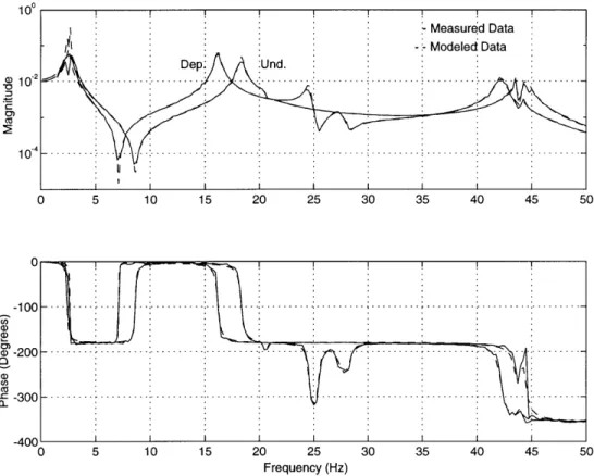
100 02Dep. Und. 10)4 1-200. --.-.... 0 5 10 15 20 25 30 35 40 45 50 -400 0 5 10 15 20 25 30 35 40 45 50 Frequency (Hz)

Figure 4.3: Frequency response functions for measured data and identified system of the testbench at location 27

output) state-space system matrix describing the dynamics of the system at the output locations. Figure 4.3 shows the Bode plots of the frequency response from one SISO transfer function, load cell (location 4) to displacement at location 27. The raw data and the identified system are included for flutter stopper deployed and undeployed models.

The quality of the fit, and therefore the identified (modal) model, is dependent on several factors. The most important of these is the frequency resolution of the data in the discretized transfer function. If the data is taken with a wide frequency spacing, then the pole locations and damping ratios may not be accurately represented in the raw data. The result is that the

(43)

system identification procedure produces a model which does not as closely resemble the behavior of the actual test piece. The identification algorithm can only be as good as the quality of the data taken.

From the identified model, the natural frequencies and modeshapes are extracted for analysis and comparison with the finite element model. This comparison is found in the following section. The modeshapes of the experimental models for flutter stopper undeployed and deployed cases are plotted in Appendix 4A, along with the corresponding FEM modeshapes.

4.3 Finite Element Model of the Testbench

This section focuses on the development of an analytical model of the testbench using the finite element modeling program ADINA. The purpose of constructing a finite element model (FEM) of the testbench is to act as a validation of the analytical modeling process for the composite spar. The testbench model is in fact based directly on the finite element model of the composite spar, which had been used previously for design decisions. If the analytical model is shown to accurately predict the response of the testbench, then confidence is gained in the analytical model of the composite spar.

The finite element mesh of the testbench model is pictured in Figures 4.4 and 4.5. Figure 4.4 is a three-dimensional view of the wire-mesh grid, which highlights the vertical region of the root attachment. Figure 4.5 pictures the different element group regions of the model. The testbench and root attachment are divided into 6 chordwise elements and 24 spanwise elements. The root attachment is modeled as a vertical plate attached to a horizontal plate, which is represented in regions 1 and 2 of Figure 4.5. The horizontal plate is split into a three-layered plate where the testbench fits into the root attachment slot, regions 3 and 4 (see also Figure 2.4). The

(44)

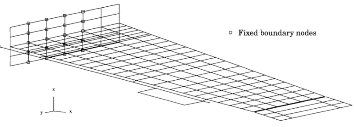
o Fixed boundary nodes

y x

Figure 4.4: Fixed boundary node locations on the finite element mesh, viewed from above and behind the trailing edge tip

remaining plate regions, regions 5 through 11, are single-layer elements representing the aluminum testbench plate. All plate elements, whether single- or multi-layered, are 4 node orthotropic elements, and have either 5 or 6 degrees of freedom at each node, depending on whether the node intersects with another type of element or not. Fixed boundary conditions are imposed for the node points at which it is bolted to the mounting assembly. These boundary nodes are highlighted in Figure 4.5.

The GVT on the testbench is done with the flap drive and flutter stopper installed. Therefore, the FE model must include these items as well. The flutter stopper is modeled as a collection of isotropic beam elements, shown in Figure 4.5. All assemblies are explicitly included, except for the latch, magnet, and position sensor, which are included by increasing the density of the frame beam elements at those locations. Both the aft (undeployed) and forward (deployed) tungsten mass locations are modeled, and the two cases are considered as separate models from this point on. Figure 4.5 pictures both flutter stopper locations, although only one position

(45)

Region 1: Root Attachment (Vertical Plate Region) Region 2: Root Attachment

Region 3: Root Attachment, Testbench Region 4: Root Attachment, Testbench

Region 5: Testbench Region 6: Testbench Region 7: Testbench Region 8: Testbench Region 9: Testbench n 10: Testbench Region 11: Testbench Flutter Stopper Deployed Flutter Stopper position

Figure 4.5: Element group regions and composition of the finite element mesh for the testbench

is used in each model. Isotropic beam elements are also used to model the flap drive, except for the flap, which is represented by a single-layered

orthotropic shell. The graphite-epoxy tubes are considered homogeneous, and the material properties are consistent with the overall properties of the tubes. The spline is modeled as a single element, and no provision is given for its axial degree of freedom. The universal joints and steel rods which connect the components together are included as part of the tubes, and the weights of these pieces are added as point masses at representative node locations. Component material properties and weights for the flap drive and flutter stopper are tabulated in Appendix A.

Testbench root

(46)

z Mt Mr x _Ms Mt Mr Ms

Figure 4.6: Bending degrees of freedom for beam elements

There are several places where certain degrees of freedom must be allowed along the drive shaft. The bending degrees of freedom at the universal joints are expressed by setting the bending moments in those directions on the ends of the elements to zero. In Figure 4.6, these are pictured as Ms and Mt. In addition, there must be a rotational degree of freedom between each bearing mount and the ends of the flap tubes, where the drive shaft passes through the bearings. This is achieved by creating a very short beam element between a bearing mount end node and the flap tube end nodes, as shown in Figure 4.7. This extra element translates the global deflection and rotation from the bearing mount to the drive shaft, but has zero torsional inertia to allow the shaft to rotate freely along its axis.

0.05"-~ flap drive

connecting element

trailing edge of spar

(not to scale)

Figure 4.7: Schematic of an extra connecting element from the drive shaft to a bearing mount

(47)

The fixed boundary conditions on the flap drive are imposed by restraining all degrees of freedom at the motor end of the flap drive, in line with the end of the root attachment.

Dynamic analyses are performed for both configurations, flutter stopper deployed and undeployed. The mass matrix is consistent, and no structural damping is included. The solution algorithm solves for the 5 lowest natural frequencies, and these are output with the corresponding modeshapes. In order to compare the finite element model with the modal response, it is necessary to create a state-space representation from the finite-element model results, from which transfer functions can be extracted. From the standard spate-space system representation

x = Ax+Bu

y = Cx + Du

A, B, C, and D are created such that

[0

I

A= ₀₂ _-2_w

B = [T _b

(4.2)

C=[c,Q c2 ] D = [0]

where 02 is the matrix of squared natural frequencies, b is a vector of ones and zeros which selects the node at which the input occurs, and cl and c2 are vectors of 1's and O's which select the output node locations for displacement

and velocity (in this case, c2=[01). Damping must be input to the model, so is set equal to 1% for each mode. The value of 1% is an acceptable

approximation using the proportional viscous damping model. From this model, transfer functions can be produced between the force input location to selected output locations, or cl can be chosen such that all 44 locations are represented. Figure 4.8 is a FEM system response Bode plot of the FRF from the same SISO transfer function as Figure 4.3. The analytical modeshapes

(48)

104 . ... :. . . - . - ' . ... : ... ... .... ... :... 0 5 10 15 20 25 30 35 40 45 50 0 -1 0 0 . .. ... ... ... ... ... ... ... -300 . ... . ... .--. .--- --- ---- ----... ... ... - --- .--.... -400 0 5 10 15 20 25 30 35 40 45 50 Frequency (Hz)

Figure 4.8: Transfer functions from the finite element model of the testbench, location 27

are shown in Appendix 4A, while the frequency response and modal characteristics are compared with the experimental results in the following section.

4.4 Testbench Model Comparison

This section contains a discussion of the two types of comparisons that are made on the modal properties of the models: qualitative comparisons, and quantitative comparisons. Qualitative methods mainly involve comparing FRFs, modeshapes, and node lines, while quantitative methods include comparing natural frequencies, as well as making a numerical

evaluation of the similarity of each modeshape.