The dynamics of moving filaments and tapes

j'.".

THE DYNAMICS OF MOVING FILAMENTS AND TAPES

BY

WILLARD W. ANDERSON B.S. Northeastern University

(1962)

M.S. Massachusetts Institute of Technology

SUBMITTED IN PARTIAL FULFILL~lliNT OF

THE REQUIREMENTS FOR THE DEGREE OF DOCTOR OF SCIENCE

at the

MASSACHUSETTS INSTITUTE OF TECHNOLOGY

~.

February, 1966

Signature of Author •••••••••••••- ...,..•...,.•••'••••••- . Department of Mechanical En~ineering Fibers and PO~Ymers D~visiorr;JFebru~~y

7,

1966 Certified by ••••••••••••••••••• _ ••••••• "-

""-Th;;i;.

s~;;~;i;~;.

Accepted by ••••••••••••• ~••••••••••••••••••••••••••••••••••••

Chairman, Departmental Committee on Graduate Students

THE DYNAMICS OF MOVING FILAMENTS AND TAPES

by

Willard W. Anderson

Submitted to the Department of Mechanical Engineering on February

7,

1966 in partial fulfillment of the requirements for the degree of Doctor of Science.

ABSTRACT

The dynamics of filaments and tapes moving at constant velocity has been studied for two-dimensional and three-dimensional boundary conditions. The equations of motion

solved are linear and include effects of tension, Cariolis' acceleration, relative logitudinal air motion, centrifugal acceleration, relative lateral air motion, and gravity. The solutions to these equations have been experimentally

validated where necessary.

The additional effects of longitudinal accelerations and dynamic buckling have been studied. The effect of a surrounding matrix on these additional motions has also heen studied. A set of twenty distinguishing parameters is included which are helpful in cata~orlzing the above motions.

Thesis Supervisor: Stanley Backer

Professor of

t'l

- I

ACKNOWLEDGEMENTS -,

I wish to express gratitude and thanks to Professors

Stanley Backer, A. B. McNamara and Dean Karnopp for their

guidance and encouragement in this work.

In addition, to Draper Corporation, Hopedale, Massachusetts,

goes my appreciation for their sunport for the initial phase

of this work and to Cohoon and Heasley, Inc., Cambridge,

Massachusetts, for their support of the final phase of this

work.

I would like to thank Professor Eggerton for his assistance

in photographing the extremely rapid phenomena of nylon filament

snapback or dynamic buckling.

I would also like to thank Professor J. P. Den Hartog for

a most important sug~estion, namely to non-dimensionalize all

of the parameters of this thesis.

Finally, I wish to thank my wife, Jane Anderson, for her

I. INrrRODUCTION

TABLE O.B'CONT EN rrS,

1

II. GENERAL VECTOR EQUATIONS

8

A. Introduction

8

B. Derinitions 8

C. Forces Acting on an Identified Filament Particle 10

D. General Vector Differential Equations

14

III. GENEHAL EQUATION REDUCTION FOR LINEAR MOTION 17

IV. SOLUTION FOR NON_OSCILLATORY BOUNDARY CONDITIONS

25

V. SOLUTION FOR OSCILLATORY BOUNDARY CONDITIONS

34

A. Two Dimensions

34

B. Three Dimensions

53

C. Boundary Layer 62

D. Practical Example of Unwinding Cone 68

VI. ACCELERATION EF}'.c;CTSAND DY".NAIJIICBUCKLING

74

A. Introduction

74

B. Accelerating Filaments

74

C. Decelerating Filaments

80

VII. EFFECT OF SURROUNDING MATRIX 99

A. Introduction 99

B. ~ropagation of Strain Release Wave 101

C. Dynamic Buckling \'Jithin the Matrix 107

VIII. DISrrINGUISHING PArlAI1I~il'EHS

i

TABlliOF' CONTENTS (cont inued )

IA. EXPEHI~lliNTATION 120

A. Filament Rotation Angle Measurements 120

B. Boundary Region Frequency Measurements 122

C. Balloon Length Measurements 123

D. Dynamic Buckling PhotoGraphs

124-E. Dynamic Buckling Wave Len~th Measurements 126

F. Experimental Apparatus for Filament Motion 126

X. SUIvlMliRYAND CONCLUSIONS 128

XI. APPENDICE~ 133

LIST OF FIGURES

Figure Title Page

1. Drag Coefficients vs. Filament Lateral Velocity

13

2. Gravity Effects, b,~ 0

29

3. Gravity Effects, b₃-O 29

4.

Fluid Stream Behavior of High Speed Yarn, b₇₎ 1 32

5.

Boundary Conditions for Yarn Winding Machinery 32 6. Amplitude Function vs. x, b₃

=

b

_s

=

0

42

7.

8.

9. 10. lla. lIb. 12.

13.

Amplitude Function vs. b~, Maximum Value Typical Machine Oscillations

Example of Circular y-z Boundary Conditions Filament Rotation

Three Dimensional ko Solution, b₇

=

1:-2 Three Dimensional ko Solution, b₇ _- 1:-4

Filament Rotation Angle Boundary Region 42

44

54

54

57

58

59

59

14.

Comparison of Boundary Layer Solution with

Calculated and with Experimental 66

15.

Frequency Measurement Apparatus 66

16a. Minimum Cone Geometry, Yarn and System Variables 69

lbb. b,'tvs. x/ro For Two Yarns 69

16c. Comparison of Relative Frequency Parameters 72

17a. Accelerating Flexible Filament .79

l7b. Decelerating Flexible Filament 79

18. Nylon Filament Snap Back

84

19. Buckling Flexible Filament 87

20. Strain Wave Propagation 90

Figure

EIST'OFI FIGURES, (continued)

Title Page

21. Wave Length Ratio vs. Impact Velocity for Nylon

!-1onofilament 90

22. Fundamental Wave Length vs. Impact Velocity (C opper vlire)

26.

Experimental Apparatus for Filament Motion (Within a Matrix) 23. 24a. 24b. 24c. 25.

27.

28a. 28b. 29a. 29b. 29c. 29d. 2ge.

Three Dimensional Buckling

~ vs. x, t = to (Within a Matrix)

Strain vs. x, t

=

.4to (Within a Matrix)

Velocity vs. t, x =

.4xo

(Within a Matrix)

8

vs.~. i' Filament Motion Within Static JJynam c

Matrix

Examples of Filament Surface Breakthrough Typical Filament Space Curve

Schematic of Frequency Measurement Apparatus Air Turbine Driven Gear Yarn Ejector

\

Air Drag and GraVity Effect b,> 1

Air Drag and Gravity Effect b_1..,1 Generation of n Lift If If Venturi Effect II

95

96 103 103 103 106 106 109 121 121 125 125 125 125 125

NOHENCLATURlt.:

, ~

a Filament Acceleration in i-direction

a Infinite Series Coefficient

n

as Material Son1c Velocity

b Distinguishing Parameter Symbol (See Section VIII)

c Lateral Wave Phase Velocity c~~ Arbitrary Constant

--:0..

d Unit Vector in Direction of Air Drag Force

f Frequency

f(s,t) Overall Filament Motion Function

few) Initial Condition Displacement Function

g Gravity Constant

g(w) Initial Condition Velocity Function

g(x) Amplitude Function (See Equation V-b)

ho Maximum Lateral Filament Displacement i Unit Vector in the x-direction

j Unit Vector in the y-direction k Wave Number

-.:...

k Unit Vector in the z-direction

Q System Length

~o Static Release Penetration Distance

~~ Cone Length

~~ Modified System Length

m,n Integers

~

n Filament Principal Unit Normal Vector

p Radial Interface Pressure

Po Stagnation Pressure of Fluid Stream

NOMENCLATURE (continued)

r Instantaneous Filament Radius or Curvature rn Linear Air Drag Coefficient

~ Amplitude of Oscillatory Boundary Conditions at x = ~ r ~~ Amplitude of Oscillatory Boundary Conditions at x = 0

o

s Lagrangian Coordinate

t Time

u Unit Step Function

~

u Unit Vector in Filament Direction --a.

u

r Unit Vector in Radial Direction

~

u_e Unit Vector in Tangential Direction v Filament Velocity

va Longitudinal Air Velocity Relative to Filament AVa Longitudinal Air Velocity

w Displacement Function x. Coordinate

X_o Strain Wave Penetration Length y Coordinate

z Coordinate

A Filament Cross Sectional Area An Arbitrary Constants

En Arbitrary Constants

CD Pressure Drag Coefficient for Smooth Cylinders

D Linear Operator

~

Db Air Drag Force Df Filament Diameter

NOMENCLATURE (continued)

E Elastic Modulus F_g Gravity Force

I Filament Cross Sectional Area Moment of Inertia J_o Bessel Function of Real Argument

K Matrix Stiffness

M Filamerit--BendingMoment

N Integer

P Filament Longitudinal Impact Force

R Distinguishing Parameter Function (See Equation V-2) R~ Limiting Ratio of Terms of Infinite Series

R Position Vector

Re Real ~art of Complex Function T Magnitude or Filament Tension To Constant Minimum Filament Tension AT Filament Tension Increase, A.T = T - To

.-::-T Filament Tension Vector

~

V~ Normal Component of Air Velocity Relative to the Filament --:...

V_N Component of Filament Velocity Normal to Pilament Direction Vs Shear Force in Filament

Yo Bessel Function of Imaginary Argument ~~ Linear Air Drag Parameter

0<", Bessel Function Argument Coefricient

~ Acceleration Function

~*

~ Deceleration Function ~ Boundary Region Angle

~e Stiffness Function

NOMENCLATURE (continued)

S Boundary Region Length

6

Small Wave Number Corrections

')'Z.)~

6c.

Displacement of Yarn ItJithdrawalPoint From Gone Tip

6~ Broken Filament Extension

€ Filament Stiffness Parameter = EI/~~A Filament Strain

e

~

Displacement in the u~-direction

~

Displacement in the j-direction Gravity Deflection

General Lateral Maximum Amplitude

Distinguishing Parameter Function (See Equation V-2) Filament Tangent An~le in x-y Plane

Constant Inclination Angle of Filament at x

=

Q

Constant Inclination Angle of Filament at x

=

0 Yarn Twist Angle

Yarn Angle on Cone Surface

~Jave Leng:th

Euler Wave Length

Coefficient of Friction Between Filament and Matrix Coefficient of Friction Between Filament and Cone Kinematic Viscosity of Air

-:lI...

Displacement in the i-direction Density of Air

Density of Filament

~

Displacement in the k-direction Phase Angle at x

=

Jl.

.'

NOMENCLATURE (continued)

Phase Angle at x

=

0 ~

Displacement in u_e- direction Cone Apex Angle

Special Modes (Hanging Chain Solution) Vector Displacement

Frequency of Forced Oscillation Relative to Moving Filament

Natural Frequency (Hanging Chain Solution) Frequency of Forced Oscillation at x

=~

Frequency of Forced Oscillation at

x

=

0

System Natural Frequency for k_o Solution With Zero Air Drag

n'

..H... System Natural Frequency for Boundary Region

Jl~ System Natu~al Frequency for'Low Filament Stiffness

lln

System Natural F1requency

I. IN~RODUCTION

This thesis is intended to be primarily a general analytical approach and secondly an experimental approach,

to the phenomena of moving filaments and tapes. The experimental anproach is limited."tb' tlhe.veriffcat16n'1of-;only the-fundamental";. results of the Analytical approach. Extensive experimental

validification of detailed analytical results is not intended. The word filament is intended to imply a yarn, string,

rope, wire, monofilament, etc.; a structure which is essentially thin, flexible and continuous with small, but not necessarily negligible, bending stiffness. Tapes are considered as

two-dimensional filaments with prim8rily the same description. The phenomena of these moving filaments and tapes form a

small related field within the sub ,jectmatter of applied mechanics. Moving filaments and tapes can be characterized

as mechanical systems and described with the concepts of mechanical engineering systems. The material in this thesis

is intended to apply within the context of Textile Mechanical Processing.

If the path of a moving filament is separated into regions between guide points on a textile processing machine, these points can be considered as the boundaries of the mechanical system. Statements can he made concerning the conditions at these boundaries and equations developed to predict filament motion and tension within the'boundaries. Examples of system houndaries are seen in machinery involved with the spinning,

the drafting, the winding, .the twisting, etc., of both staple and continuous-filament yarn. In these cases the system

includes both the region and the filament within the region. The spinning balloon, the overend ~nwinding balloon and the filament space curves associated with high frequency yarn traversing mechanisms are well known examples of yarn systems generated in the average textile mill.

The literature contains numerous reports related to the subject of moving filaments. However, in general, each. of these renorts has confined its attention to a specific

phenomenon of filament motion within a specific textile machine, rather than to the overall phenomena of moving filaments

within general system boundaries. The assumptions made in these previously pUblished reports and papers have been too restrictive in the sense that the results cannot be applied to situations which are not completely similar. It is

admitted, however, that there are published analyses which move further into the detailed mathematics 01' a single moving

filament situation.

Hannah (11), Mack

(23)

and Crank

(24)

have studied in detail the nonlinear equations that apply to the cap and ring

spinning systems, commonly employed in textile yarn processing. They have neglected filament stiffness~and tangential air drag' and have considered the'surrounding air as stationary.~ Their; numerical results have been obtained from the direct numerical integration of their developed differential equations. Hannah (11) has dealt only with cap spinning and by making simplifying assumptions about air drag forces, she has expressed her

-2-results as a function of a single cap spinning parameter.

Mack

(23)

has made a more exact formulation of air drag and obtained results which apply to both cap spinning and ring

spinning. His results are expressible as functions of two

parameters, an air drag parameter and a tension parameter.

Crank (24) has also investigated the equations which apply to

cap and ring spinning systems. He has, however, included the

effect of longitUdinal yarn velocity, commonly called the

If Coriolis Effect II. For zero longitudinal yarn velocity his results are also expressible as functions of a tension parameter

and an air drag parameter, similar to those of Mack

(23).

DeBarr (3)has summarized previous theoretical and analytical findings for cotton ring spinning systems.

Padfield (4)has examined the specific equations of yarn motion for an overend unwinding yarn package. She has

numerically integrated her derived differential equations and

the results are presented as specific plots of yarn space

curves. Padfield (10)(12) has discussed the boundary conditions

at package surfaces, such as are used in this paper.

Brunnschwei1er (20)(21) has also dealt with overend unwinding

yarn packages by measuring yarn tension and photographing yarn

space curves. This study is unfortunately only experimental

and does not try to validate a specific theory.

There are, of course, many linear solutions for oscillating

strings and beams. But of these only Sack (19)has included longitudinal velocity in solving the differential equations of

A. general analytical-approach should begin 'with a" general filament model. The equations which describe this

general model must be complete in order to predict the behavior of an actual filament. Therefore, forces from filament tensiOn;) filament shear, gravity and air drag are included. A point

on the filament is identified as en infinitesimal particle of constant mass. The above forces are then summed and equated to the rate of change of momentum of this infinitesimal mass. This summation leads to the ~eneral vector differential equation for a moving filament.

This ~eneral vector differential equation can be written

....

in terms of a filament position vector, R(s,t). The position vector specifies the position in space of the filament particle, with respect to a fixed inertial reference frame. The

coordinate, s, specifies the distance along the filament from a point on the filament, the position of which is knOl~ at

some reference time. It is possible to choose a specific position vector in order to describe any type of filament

motion desired. The position vector can contain a description of the net, or average motion, of the filament plUS a statement of the perturbations or small deviations from this average

motion. This makes it possible to derive governing differential equations for specific net motions and boundary conditions in a way such that the initial simplificati.ons can be made from physical judgements.

The general vector differential equation has been examined extensively for the case of linear filament motion. The term

-4-linear filament motion refers to filament motion which is essentially straight line travel between two boundary points with the addition of small perturbations in the two lateral directions. Linear filament motion is sufficient to describe the practical textile processing situations described above.

The results of this examination or the differential

equations of linear filament motion are nresented as simplified equations, which can be used to predict the paths through

snace of actual filaments. 'These equations are formulated in terms of dimensionless combinations of variables which refer to the relative magnitudes of filament stiffness, air drag, gravity, etc. These dimensionless parameters can also be used to predict identifying quantities such as the number of

filament balloons (in an unwinding situation), the magnitude of'the filament rotation angle in a given balloon, the length of the boundary "stiffnessil

region versus the flexible region in a given filament, etc. They are also logical correlation parameters 'for ,experimental or numerical data.

For moving filaments which have small, but not necessarily negligible stiffness, a concept of a boundary stiffness region is introduced. Equations are developed which allow a prediction of the length of this region. The equations describing the

linear motion of flexihle filaments are then modified using this length.

The linear equations assume constant overall filament velocity, v. There are practical situations, however, where the displacements and strains of accelerating or decelerating

filaments become imnortant. These situations include the transient behavior of filament systems during the start up or shut down of processing equipment. They also include the dynamic buckling which occurs when a filament, moving at high speeds through a machine guide, is sUddenly stopped at one point along its path. Equations have been developed to

permit prediction of the time dependence' and the mode shapes of both the stable oscillations corresponding to accelerating filaments, and the unstable deformations of decelerating or dynamically buckling filaments.

The effect that a surrounding matrix of solid material can have on the dynamics of filament rupture is also examined. The equations develoned nrovide, to a limited extent, a

quantitative picture of the internal dynamics of a breaking yarn. The internal dynamics of a breaking yarn is important

in determining yarn strength and strength has an important effect on process efficiency.

It is felt that this thesis can be used as an aid to textile machinery designers, since it allows an accurate prediction to be made as to the actual filament motions and strains that take place as a result of machine-material interactions.

At the present time when one designs a piece of machinery through which a filament or a tape will pass, almost all of the desi~n effort is involved with factors affecting machine life, cost, reliability, etc. Little consideration is ~iven to the interaction hetween machine and filament. This can lead to situations where a filament is modified in some

-6-undesIrable manner as a result of nassing through a machine.

An example of this is the progressive drafting of cotton yarn

that takes place as the yarn is being wound on a drum winder.

It has been found that rewinding the same yarn package as few'

as five times on certain drum winders causes a sufficient

amount of drafting that the yarn may break in several places

(30). A second example is the package surface instability (shellorf) that occurs vThen yarn is drawn overend from a

yarn cone at sufficient withdrawal speeds. Whole yarn loops

slide down the cone surface leaving the package at one time

and causing a disruption in smooth flow of yarn from the

package. ~fuen one tries to use such a cone for the filling

yarn on a shuttless loom the speed of the 100m becomes limited

by the speed at which this instability occurs (31).

It is suggested that the application of the solutions of

this thesis toward specific problems such as those ahove is a

logical i.nitial step in the direction of reducing undesirable

II. GENERAL VECTOR DIFFEH~NTIAL EQUATION

A. Introduction

The first portion of this thesis is devoted to the examination of a general model of a moving filament. The equations which describe this general model must be complete in order to predict the behavior of an actual filament.

Therefore, forces from filament tension, filament shear, gravity and air drag are included. A point on the filament is identified as an infinitesimal particle of constant mass. The above forces are then summed and equated to the rate of change of momentum of this infinitesimal mass. This results in an equation, called the general vector differential

equation for a moving filament.

B. Definitions

In order to present the derivation of the general vector differential equation several definitions must first be

established.

Filgment Particle The filament particle is defined as the infinitesimal mass, ~~AAS, which exists at a point on the filament defined by the coordinate, s.

~

Position Vector

=

R(s,t) The position vector specifies the position in space, with respect to a fixed inertial

reference frame, of the filament particle. The coordinate, s, specifies the distance along the filament from a point on the filament, the position of which is known at some

reference time. The derivatives of this vector have the

-8-following properties.

~

~R. .

~t(S,t) = Velocity of particle s at time, t.

~ ~"Z..R

ht~(s,t) = Acceleration of particle s at time, t. -a...

~:(B,t) =~(B,t)

= Unit Tangent Vector (in filament d ire ction) at s.

~

>::.2.. R ~

r ~s~(s,t)

=

n(s,t)

=

Unit Principal Normal Vector to the filament, where r is the instantaneous radius of curvature of the filament at s at time, t.

-Jl.,

-a.( , ....~R()

Tension Vector

=

Ts,t)

= ~

s,t The tension in a filament acts in the direction of the filament axis and can be represented as the product of a scalar magnitude, T, and

~

~ ~R

the unit vector, u = bS.

Coordinate System

--Y (J )

-1lK.)

This right hand cartesian coordinate system will be used throughout unless noted. Gravity will be taken as acting in

.-....

C. Forces Acting on an Identified Filament Particle. ~ Filament Tension, T ~ -=:a.. = (6T ~ + T ~"J..R)A

o

S b S ~s2. S ~

Filament Shear Force, V~

This force is left in general form and will be considered in greater detail only in the specific cases where it Is

significant.

--=--Gravity Force, F~

~

Air Drag Force, D

As a filament moves through the air or any viscous medium it feels a net drag force associated with the lack

of pressure recovery behind it. This type of drag force is discussed for both continuous-filament yarns and staple fiber yarns in Chapter

3

of Reference

3.

This reference

-10-~

direction of

Vb

is a function

~

~~' and the unit vector in This can be shown as follows • states that if the ratio of lateral yarn velocity to

longitudinal yarn velocity is large then continuous-filament yarns behave substantially as smooth cylinders with the air drag force acting in a direction normal to the filament axis. However, for staple fiber yarns, the air drag is greater than would be ex~ected on this basis - the effective yarn diameter being approximately

50%

greater than the actual yarn diameter.

This occurs because portions of fibers protrude from the yarn surface into the air stream, spoiling the flow.

If the ratio of lateral yarn velocity to longitudinal yarn velocity is not large then the air drag force has a component along the" filament axis. This component does not influence lateral yarn motion directly, but affect~ tension -which in turn influences lateral motion.

The general filament model of this thesis considers that forces from air drag act normal to the filament axis and obey the standard equation for smooth c~linders. The normal

component of air velocity relative to the filament is given

~

the symbol, V~. The magnitude and of the filament particle velocity,

-3000 the filament direction, ~ = ~~.

...a..

~ bR

~u=

lrS

= Unit Tangent Vector (in Filament Direction)

Filament Particle Velocity

~

V_w = Component of Filament Velocity Normal to Filament Direction at s.

Since

(11-1)

~

The absolute value of V1> is most easily found by noticing

~ ~-:....

~R ~R oR

--'-that (0 t ..0 8) ~s' and -VI) ar~the tHO sides of a right triangle whose hypotenuse is ~~. Therefore:

:. V1)

~ -:so.. -::....:....

oR.

oR

= Va.+(~R. ~R)a

ot

0 t b cbt 68

-s.. ~ -'- ~

-.300",

I

~

R 0 R 6 R ~ R~}

'/2-=\

VI) =

f (

b t •

bt) -(

bt •

bS

J _j

The drag force can now be given the magnitude,,' V2.

AD = C ~9 D D AS

1) 2 f

CD is a function of Reynolds Number and.-1s given in most .standard fluid mechanics ~exts. Specifically, it is given

in Reference 6.

Yet

is the density of air and D-f is the filament diameter.

'The direction of the drag force is the same as the

-...

direction of

""0.

Therefore, if the unit vector in this

~

~ V

direction is taken as d

=

V:'

the drag force vector can be expressed as:

S_{inca C~ is a function of Reynolds Number, Rey=}

!lQr.

_{v '} where V is the ktnematic v1.scoslty of atr, it can be seen that for a given filament the magnitude of the drag force

-12-is a function of V_D only. For low values of V

_o

the drag force is proportional to VOl while for high values of _VD the drag force is pro~ortional to

V~.

This velocity dependence is shown in Figure 1 for a hypothetical 20 mil filament

moving through air at standard temperature and pressure.

3

100 rl) ;t. 107 2 (lbt. see) _C n ft;z. 1 0 O. ':2 ",:,1 .0 .1 .2 ₃ Log Vt> '(rt/sec)

Drag Coefficients vs. Filament Lateral Velocity ~IG. 1

r_D is defined _{as the drag force per unit length of filament} per unit of normal relative air velocity and is expressed by the equa.tion,

~II-3)

Figure 1 illustrates that for a typical continuous-filament yarn the drag force is proportional to VD(constant r_n) for values of Vb~ 0.1 ft/sec. For values of Vb> 100 ft/sec the drag force is proportional to V~ (constant

CD).

It is

unfortunate that the range of practical interest lies between these two values of Vb and therefore, for most situations the drag force cannot be accurately modeled by a constant r

D or a constant CD- However, when considering air drag in connection with the linear equations to be discussed later in this thesis, the air drag force will be assumed proportional to V

_ne

It is therefore, necessary to use an average value far rD. The average value of ~ ,should be chosen so that it

yields the actual energy loss per cycle. If the drag force

2-is ~ctually proportional to V_D the correct average value for harmonic oscillation is:

r

=

.85Maximum Drag Force per Unit Filament Length D Maximum Filament Normal Air Velocity This value is calculated in AppendiX 1.

acceleration.

The terms in this equation refer to forces from variable tension, filament curvature, bending stiffness, gravity, air drag and rate of change of filament particle momentum (mass times acceleration). If the tension is considered constant and shear forces are negligible then the equation becomes:

-14-(II-.5)

If forces from gravity and air drag are also negligible the equation is fu~ther reduced to:

c'2. _ T

- ~f.A (II-6)

where c is the well known phase velocity, a most important variable in any discussion of filament motion.

The general vector differential equation has been

~

derived in terms of the general position vector, R. It is therefore possible to choose any specific position vector in order to describe any type of filament motion desired. The position vector can contain a descrtption of the net, or average motion, of the filament plus e statement of the

perturbations or small deviations from this average motion. This makes it possible to derive governing differential equations for specific net "motions and boundary conditions in a way such that the initial simplifications are made from physical jUdgments.. As an example, consider the perturbations

of an idealized horizontal lasso from an essentially circular path. The position vector is given as:

Where "X, ~ and "(are IIsmall" displacements in the tangential, radial and vertical directions respectively; v is the net

~ ~ --3000.

filament velocity and ue' u~ and j are unit vectors in the tangential, radial and vertical directions respectively.

If these small displacements are taken as zero the overall stability condition for this filament configuration can be found. Considering Equation 1I-6 to be applicable for this simple example and substituting the above position vector with the small displacements taken as zero, one finds that v must equal c for stability (T

=

~~AV4). This defines the net or average motion of the filament and substitution of the complete position vector yields three equations which define the three nsmall" displacements from this stable configuration.

This is a simple and well known example and illustrates the use of the position vector. However, there are many other stable configurations from which there can be small perturbations worthy of investigation. The nosition vector which defines an essentially straight line motion is the one of most practical interest in industrial processing of

filaments, and

so

the rest of the thesis will be devoted to its examination.

-16-III. GENERAL EQUATION REDUCTION FOR LINEAR MOTION

The practical aim of this thesis is to define quantitatively, and to a large degree qualitatively, a number of flowing yarn, wire, and tape situations. This can be accomplished by examining the solution to the general vector differential equation for a position vector where the net or overall motion is essentially straight line motion. This position vector can be defined as follows:

~ ~ --"'- ~

R(s,t) = (f (s,t) + ~)i + 4(j +

ee

k (III-l)

In this equation '1( and

'f.

are the ItsmallII displacements

in the y and z directions of a filament particle moving in the positive x direction with an overall motion defined by f(s,t) and an additional "small" displacement defined by ~. This case is considered as linear motion since the filament deviates from an essentially straight line path in the

..a..

i-direction. The ratio of dx to ds is therefore taken as 1. The'function"'f(s.t) will be given the value vt + s, in this

section,where v is constant. This further limits the motion

~

to essentially constant average velocity in the i-direction.

-In order to understand fully the phenomena of moving filaments, it has been found necessary to include the effects that air drag, filament stiffness, filament momentum and

gravity have on the motions involved. Tension remains the predominant filament control force for the cases considered in this section. But situations, either caused by extreme boundary conditions or by extreme material properties

require the inclusion of stiffness, air drag and gravity to explain deviations from the predicted results of the simpler models. The winding of glass or metals or large polymer monofilaments represent the case of extreme material

properties, while the unusual characteristics of filament motion near guides at high speeds are examples of extreme boundary conditions.

The general vector equation as defined in Section

II

is:

~

Substitution for .the i direction motion yields a one dimensional wave equation for the deflection,~, as measured from the moving reference frame.

a'2. =

-5

(III-2)

This equation refers to the actual propagation along the filament of the strain (~~) or tension (EA~~). This

propaaation takes place at the sonic velocity of the material,

as.

The ratio of as to the transverse wave velocity, c, 1s:

h = (~)~ = (..l.)~

c ~ E.-F

Therefore, if the average filament strain, e~, is small, the propagation of tension waves can be neglected in solving for the lateral displacements,

1

and~. Therefore Equation

III-1

can be simplified to:

~ R(s,t)

=

--"'- ~ ~ (vt+s)i +'1'3 +

ee

k

-18-(III-3)

The normal component of air velocity relative to the filament can be expressed as follows:

The components V_DX' Vf>y' and V1)~' are found by referring to Section II, Equation II-I, where it was shown that:

(II-I)

~

Substitution of the position vector, R(s,t), into this equation yields (neglecting second order small terms):

The velocity, v, in the above equation refers to the velocity of the filament relative to the reference frame. If the air is at rest with respect to the reference frame, then the above equation is correct. However, the movement of the filament can develop a flow of air in the direction of net or overall filament motion, which in this case is the ...boo.

i-direction. Therefore, using the average filament velocity, v, in the above equation causes an error.

By introducing the term, vq' which is equal to the

~

actual net filament velocity less the induced i-direction air flow velocity, the above equation can be written more

correctly as:

(III-4)

It is now necessary to express the air drag term in Equation'II-4 in a linear form. This is done by using the

linear air dra~ parameter r_D, previously discussed. Referring to Equations 11-2 and 11-3:

Therefore, Equation 11-4 can be rewritten as (noting that the tension is considered constant):

~ -.30..

T ~"2.R + ~Vs _ Or_gA~j + r

V

=

~s~ ~S.)T ~ b (111-5)

The filament shear force, V_S1 can be considered as the variation in bending moment along s. Since the bending

moment is directly related to the local filament curvature it is possible to say:

~

This holds true for all magnitudes of position vector, R, for a linear elastic material. Now substituting the position vector under consideration (Equation 111-3):

For small curvatures superposition holds.

~

.".). V. =-EI

~..q~r-

EI

~k

bS ~ 81 b s<4 (111-6)

Having simplified filament tension, filament air drag force and filament shear force, it is now possible to

-20-~

substitute for R (Equation !!1-3) in Equation III-5, .separate it'into two equations and rewrite in simple form.

~

For the j-direction:

~

For the k-direction:

(111-8)

Foi the boundary conditions considered in the following sections, the lateral velocity of the filament varies

harmonically with time. Thus in order to linearize the velocity dependence of air drag the constant value ror rp

must be chosen as shown in Appendix I so that the energy loss to the air for actual air drag is the srome as in the model. This is not a good approximation, but it will do no real harm to the solution since it Is only an error in a second order effect. The linearized equations are therefore:

~

For the j-direction

(I1I-9)

~

For the k-direction:

(1II-:ltO) where

(Note:

e

=

EI

=

Filament Flexural Riiidity ~A Filament Mass per Unit Length

The choice of E is to point out that this parameter

c =

vi

T: = Lateral Wave Velocity ~+

~D= ~

=

Linear Air Drag Parameter

The boundary conditions to be considered occur at points which gene~ally move \lIl1th respect to the filament. If the

filament is considered to move toward positive x then points of fixed x - where some boundary conditions of forced

vibration may be taking place - move toward negative s. This is simply expressed as:

s = x - vt

Therefore, a wave solution for

1,

for fixed x boundary conditions would have the form:

where ti(wot + lex)

'1=

~e + ~(x)

:!:i

(U.)t + ks) =

roe

+ ~(S' + vt)

w

= OJo+ kv (III-11)

Substitution of this wave solution into Equation 111-9 yields two equations:

4- "2.(:L '2.) ( 2.

€. k + k c -v +k -2wov+iocD( v-v~ ))+ (-UJo+io<.1)~Q) =

E. ~ _(c'L_V"')

t~

+~.(v-v..)

ti3

+ g

=

0

o

(III-12)

(III-I)

Equation III-I) is reduced to derivatives with respect to the ar~ument, s + vt = x. It is also possible to derive an

equation similar to Equation 11I-12 'for".thedisplacement in

...:lo.-the k-direction,

if.

But this is not considered necessary

-22-since the equation 'Would be identical to Equation 111-12. Equation 111-12 can be further simplified by introducing five dimensionless parameters. These parameters are:

(Stiffness Parameter)

(Coriolis Parameter) (Longitudinal Air Motion

Parameter)

(Centrifugal Force Parameter)

(Lateral Air Drag Parameter) _ 2 uJgVC?fAJl. T- ~~Av'2. = r)) (v-Vq

Hl.

T..;. ~fAv:z.. b~ - -ba. -

-The nhysical meaning of these parameters is discussed throughout the text and summarized in Section VIII. They refer, in order, to the effect that filament stiffness, Coriolis' acceleration, relative longitudinal air motion, centrifugal acceleration and relative Ie.teral air motion have relative to net filament tension, (T- ~FAv~), on the

motions 01" the filament. The system length, .2, is introduced

as a convenient way to non-dimensionalize these parameters. Equation 111-12 becomes:

(111-14)

A good physical interpretation for kQ is that it is the numher of waves that exist within the system boundaries, multinlied by the constant, 2rr.

Equation 111-13 can be rewritten by introducing:

b

=

gQ =

Equation 111-13 becomes:

1Y

b (~)

I Q

(111-15)

Where the Roman numerals refer to differentiation with respect to the argument, ~ = (s+vt)/~.

In the following two sections Equations 111-14 and III-1S are investigated for specific boundary conditions and for

varying magnitudes of the parameters, b.~ b~.

-24-. IV-24-. SOLUTION FOR NON _ OSCILLATORY BOUNDARY CONDITIONS

When a filament is moving horizontally at high speed (hundreds of feet per second) between two guides it might at first appear that the effect of gravity on the motion of the filament in the region between the guides, would be considerably reduced from that at lower speed. However, exactly the

opposite occurs.

It will be shown that the II effective tension II or the value of tension which acts as a controlling and limiting variable with regard to filament motion can be expressed as T- y~Av2.. When this II effective tension II becomes small, bending stiffness and air drag fo!'ces become important in

controlling gravity deflections.* For relatively flexible filaments (yarns, thin tapes) the control forces come

predominantly from surrounding air motion, while for relatively rigid filaments (monofilaments, metal wires) the control

forces are caused by the bending stiffness of the filament itself. But, in either case, some mechanism other than

tension must take over in con~rolling the motion between guides and it is the aim of this section to find out what this

mechanism is.

Refer to Equation III-IS:

(II1-15)

~~~

These are, however, the predictions of a linear theory and Jdo not hold for appreciable displacements.

"1f.

This is the governing equation for~, for boundary conditions, at fixed points in space (; = 0, ~ = ,1), which do not vary

with time. The input force is, of course, .gravity (b&). The

.)~

boundary condttions are stated simply as":

Now a.ssuming: r r ~ (0) = ?f (0) = "1(1) ='1{ (1) = 0 .Q. Jt .Q 1..

(IV-l)

(IV-2)

it is possible to reduce Equation 1II-15 to:

(_{b, D -}3 _{D + b} "11

3

)T

= 0

where the D refers to a dimensionless operator.

(IV-3)

The equation for D is actually the reduced form of the general cubic

equation and'D can therefore be stated as:

D,

=

A + B D2. =

_-2

A+B + A-B

F

2 D'3 -

--

A+B₂

_-2

A-B

F

where and A = {_ b3 + l{b.a2.. lb, bl 4 B =

(-..h - -!.(bf

2.b1 b,

For the case where b_l b'32..) ~, one obtains one real and two

conjugate imaginary roots. For the case where

bIb; (~.

one obtains three real, unequal roots.

Thus it is seen that superimposed on the linear term of

~~The subscript g will not be carried further.

-26-Equation IV-2, - b~~, there is an additional displacement, b3 Jl

~. The nature of ~ varies with the magnitude of b_l b~ •

~ R

When b_l b; ) ~. ~ changes in nature from exponential to

harmonic. This corresponds to a physical situation where the ef1'ects of forces arising: from stiffness and air drag exceed those arising from effective tension.

It is possible to go ahead and solve for the boundary

conditions as stated and then reduce the equation mathematically to examine each effect. But this requires extensive algebra

and is impractical. The problem is more logically examined from physical considerations.

By letting b_l ~ 0, the fourth order dependence drops out

of Equation 111-15, thus making it simple to see what happens at high speeds for flexible filaments under the influence of gravity. The differential equation becomes:

where ~-:c - b_{3 {-}Jl.} - b₍₎ = 0 ~-(a) =

""

-(1) = 0 i .Q

{IV-4}

This equation and these boundary conditions yield: (b"x)

"'=-

b.

P~_

e 11. _-1

l

_(IV-S)

JJ. b₃ ~ b₃ e -1 4{.,.QX b₃ -1 ) vlhere ₌ _ b.

fln(6

-1)+ b.3 .D. b.3~ b3 b3 e -1

(IV-6)

where

"'1",_"

=

_ ~

=

-

S\AgJ1.

o

8

(T- ~~Ava..)

For b~) b~: (IV-7)

where bE.

=

- bs

Equations IV-5, IV-6 and IV-7 are plotted in Figure 2.

The initial low velocity configuration is a parabola, with

'x

the point of maximum deflection occurring at,R.

-:=

t.

As the velocity is increased, the ,point of maximum deflection moves

toward the downstream end, (~ = 1). When the filament

velocity, v, reaches the lateral wave velocity, c, the point

of maximum deflection has moved all the way to the downstream

x

end, Jl

=

1.

As seen in Figure 2, as the filament velocity approaches

its maximum value the curvature of the filament at ~

=

1, beco~es quite large and filament stiffness can no longer be

neglected. It also cannot be neglected when the value of b,

is high (metal wire, heavy monofilaments). It is thus

necessary to examine Equation III-l.5 when b ~-+ O. The

differential equation becomes:

where

(IV-B)

This equation end these boundary conditions yield:

. x x x 2& J2 ( 0 )

~ b

G {Slnh6 - S cosh

s

-1 jfsinh6 - cosh, +1

J1. - -

2"

i) + D R 2& ~

"6

"&

sinh~ -

-:r(

cosh&, -1)

+(~)l

(IV-9)

where _{~ =. b}l112-J. = Boundary Region Length (to be discussed in Section V-C)

-28-x=o

x

X=.£

-..---r----II.---:::r---t ...V v INTERMEDIATE EQ.nZ'-5 FIG. 2 GRAVITY EFFECTS, b,"" 0

X=o

X

X=£

- ...---I.-~-I~---~r---"l~ V v -"1 FIG. 3 GRAVITY EFFECTS, b 3,.., 0

-29-For b,

«

1: where For b,

»

1: where

(IV-IO)

(IV-II)

The filament is thus seen to move from a parabolic shape at low velocity (b_l

«

1) into a complicated exponential and parabolic curve and then become the II second order parabola II

or regular beam shape at high velocity (b,'» 1). See Figure 3 which plots Equations IV-IO and IV-ll.

The variable, S J introduced above as the boundary region

length, is derived and fully discussed in Section V-C. It is necessary, however, to explain here, that it refers to the length of filament, modeled' as a massless beam, that extends from the system boundary to a point where the remaining

filament can be considered as completely flexible, but of correct mass per un! t length. Thus, for

b

«.Jl

(b,

<.<

1) the filament behaves as a flexible string. However, for ,"»).Q

(b, )

>

l) the filament behaves as a stiff beam.

Having the deflection curves for stiffness with zero air dra~ and for air drag with zero stiffness it is possible to compare the two and determine for what size filament the two effects are the same. This has been done for reasonable values of all parameters (See Appendix 2) and it was found that for monofilaments of 10 mil diameter the two effects are comparable. This diameter is considered typical.

'-30-It is unfortunately not possible within the scope of this thesis to investigate these solutions for values of

overall filament velocity, v, approaching the limiting values of lateral wave velocity, c, since these limiting values can be two or three thousand ft/sec. It is expected, however, that textile processing machinery will begin to approach these values at some future date.

The last comment made in connection with this section is concerned with the notion of the overall filament velocity, v, being greater than c. If the parameter, b_l = ~=n Equivalent Mach Number H is introduced, this notion is expressed as the Equivalent Mach Number being greater than one. Physically this means that the tension is lower than the momentum flux

2.,.

of the filament, ~~Av I and therefore does not control

filament motion. Figure 4is a photograph of a cotton yarn forced to " flow n at approximately 1.50 ft/sec by a driven

set of gears. The yarn is pushed out to the right away from the gears. The photograph was taken in a semi-dark room with the aid of one flash from a Strobotac. The overall motion is evidenced in the envelope of multiple yarn configurations, while one specific configuration is in focus. The behavior

of the yarn is similar to a fluid stream, as evidenced by the deflection of the yarn at the plexiglass plate. Reference is made to Figure 29 of Section IX which contains other examples

of this type of yarn motion.

Thus, filament speeds greater than c are certainly possible - but what happens ~s that downstream control is

FIG. 4

FLUID STREAM BEHAVIOR OF HIGH SPEED YARN b₇> I

y

1

v ---( TRAVERSING MECHANISM '=---" PACKAGE FIG. 5

BOUNDARY CONDITIONS FOR YARN WINDING MACHINERY

-32-lost. If v is forced to be greater than c it must occur by some upstream mechanism - such as pushing the filament with

an air jet or high speed rollers as was done in the experimental setup of Figure 4- Then the filament behaves as a fluid stream, and if the stiffness is low (yarn) it will deflect from

boundaries and create stagnation pressures as is ShOl~ in

Figure

4.

This cannot occur if the yarn is II pulled dOmlstream It

V. SOLUTION FOR OSCILLATORY BOUNDARY CONDITIONS

A. ~

Two Dimensions

~ ~

The lateral motions (j and k-directions) of moving filaments are usually much more complex than the simple

gravity deflections just discussed. The additional complexity is usually caused by periodic displacements or forces acting on the filament at points along its path. In order to

examine these additional lateral motions the path of a moving filament must be broken down into regions between any two such points. These points can then be considered as system boundaries and statements can be made concerning conditions

at these boundaries.

The boundary conditions for a situation of linear motion usually include harmonic oscillatton. And if the oscillation

is not harmonic, but periodic, the boundary conditions can usually be represented as an infinite number of harmonic

oscillations summed in a Fourier Series. Examples of harmonic motion would be the spinning balloon or the overend unWinding balloon, while a typical periodic motion would be represented by the filament path of the many traversing mechanisms that

exist in winding machinery. Another common periodic force is that caused by friction chattering induced by stationary

guides.

In order to cover as many of these examples as possible, the boundary conditions for this section have therefore been chosen as general as possible.

-34-The bounda~y conditions for harmonic displacement are:

~(O,t)

~~ .v.

?/(l,t)

=

~o

=

ro _{sin(w: t + ~), sinwot}

Jl. Jl. Jl

(V-1)

~""7 -'~ cos (\).)~. i5) , ~~ (~ t) AX(O,t)

=

en

₀ t + = eocoswot ~ x ' ~

The boundary conditions for the k-direction will be given later in this section, when three-dimensional motion is discussed. We shall limit the discussion here to displacements in the

-

j-direction because the equations of motion for the two lateral directions (y and z) are uncoupled and can be solved

independently.

Two-dimensional considerations are enough to describe the dynamics of moving tapes since tapes usually have stiffness ratios, for the cross directions, of many tens of thousand •• However; it must be mentioned that the ft virtual mass pel:'unit

length" of a tape is greater than its actual mass. This effect is a consequence of the relatively large local mass of air that moves with the filament.

In ol:'del:'to investigate the lateral motions of flowing filaments forced by the pel:'iodicboundary conditions of Equations V-I - it is necessary to solve the wave number

equation (Equation III-14) for the traveling wave discussed in Section III, i.e.,

4 :a.

b, (k..l) + (kl ) +(b:L+ib3 ) (k 12)+(b4+i b s) = 0

The general quartic equation, can be solved using Ferrari's method. But this method involves finding the three roots of

a cuhic equation; then, with each of these roots, reducing the quartic to a~quadratic; and solving the quadratic. Since the

coefficients in the above formula are complex end the method itself is extremely lengthly (even for real coefficients), no attempt was made to use it. Instead two approximate solutions

ar~:r'examined. "

The first approximate solution is for filaments which have very little bending stiffness (b, is small). This

solution was not carried through to completion because of the extreme amount of algebra involved and because, as will be

shown later in this section, it is possible to use a 11 boundary

layer 11 or in thls case boundary region concept for moving

filaments possessing small bending stiffness. This first solution is outlined as follows:

Let k_o be a root of the wave number equation (Equation I1I-14)' for zero filament stiffness (b, = 0).

(V-2)

where = -b_+R cas

8...+

i -b~+R sin 9_ 2 2 R = + ((b '2. b '2- )2..

4 (

)2.. )~ - -;a.. -4 4 -b₃ + ' h,.b₃-2bs

Now let there be one solution of the form:

,

k \ ~ = kC)Jl.(1 + 6. )z. ,

and one solution of the form:

where _f>, < < 1

where ~« 1

'1.

-36-Substitution into Equation III-14 yields:

( bl (ko.Q.)-4

)!

kill. =

ka1l.

1 - (k_at)2. +

(b:z.

+ib.3) l-k_oR/2) kjLt = !ib.-~

=

'!:i

.R

6

(V-3)

(V-4)

These are the four required wave numbers for Equation II1-14 when filament stiffness can be considered small (small ~ ).

The first wave number,

k.,

is a correction of ka. The correction is obviously related to the magnitude of b_l (filameht stiffness) and is zero when b, 1s zero. It can be considered an increase in the It system wave length tl (or a II stiffening II

of the system) since, by definition, a decrease in wave number represents an increase in wave length. This is a

minor correction, however, since kais only slightly decreased from ko•

The second wave number, k~, is more interesting since it represents an additional exponential displacement of the filament, with which it is possible to correct the ko solution for boundary conditions of slope. The magnitude of k2- is the reciprocal of 6, mentioned earlier as the boundary region length. Thus the amplitude of the stiffness correction varies directly with the size of the boundary region. As mentioned, this concept is fully discussed in Section V-C.

The ko solution will be carried through to completion, however, because the model for this solution represents the majority of moving flexible filament situations. The boundary conditions for slope at x/~

=

0 and x/~

=

1 are ignored,

this is as follows:

First, solve for the boundary conditions (Equations V-I) with tt_o-~t-= O. An example of these boundary conditions would

be the yarn winding machinery depicted in Figure

5.

Here 'the yarn entetts through a field guide at the left (x

=

0),

then moves thttough a traversing mechanism at the right (x =Jl ) • The displacements in this figure are exagerated to illustrate typical deviations from straight line flow. The solution is undertaken by separating the complex exponential representation

of

7

into two functions, one representing the usual spacial mode (or a wave function traveling" relative to the filament

at velocity, -v) and the other considered as a correction function to make the product of the two a solution of the

_ib'2. e 2 c

=

c:ai :L 2 _ b:s c....= &e

2

c ~ J2.' 4 where

This function fits the boundary condition at ~

=

0 (or s=-vt)

~

namely ~(O,t) = O. In order that it fit the boundary condition at~=l (or s=R-vt) let:

ib2. - -c3i e 2, c. -

-2-(V-6)

Equation

V-5

can now be more simply expressed:

f

.

.

b3(~

-1))

:!

= g (x) 1:'0 sin(w t-b (1- ~))

1

f

e 2 ~

fl. . Jl

0"

~

S

l

(Note: The amplitude function, g(x), is found by taking the

-38-real part of."the product of'c₄ and the amplitude function of." Equation V

-5. )

where

+ cos blsx/Jl. cos bas sinh bu. X/l sinh bu.

sin~b'5 cosh:l.b_ue+ cos~b.~ sinh7-b,G.

b = RsineR

\to 2'

b = -b2.

rT 2'

For b~

=

b~

=

0 (zero air drag) the solution ~educes to:

0/ = ~ sin b\1~xIR sin(w t-b (1-.!.))

.Q R sin b,s 0 I,. R.'

b = woo/c

'8 l-V7-/ c2.

(V-7)

Equation

V-7

has been published previously

by

Sack

(19).

It is easier to understand this solution by rewriting b" and b_ls in terms of."the natural f."requencyof the system,J'L •

This concept was discussed by Skutsch

(28),

however its

derivation is included here for sake of completeness. It is written as:

Physically,JL can be interpreted as follows. Consider the case of a flexible filament moving through two fixed guides

a. distance .Q. apart. If a posittve lateral disturbance is

initiated midpoint between the guides it will propagate in both directions. The disturbance will then be reflected at

the' gUid'es and return'towards the midpoInt but. wi th negative sense. It will pass through the midpoint and be reflected at the opposite guides and again return to the midpoint, but this time with the initial positive sense. This is seen in

the following figure where only the initially upstream wave is considered. ~=l .R Displacement At = Il/2 c-v ~ _ 1 ~ - 2" Direction of Initial From ~

=

.L ~ 0, Jl 2" Upstream .-- - Downstream

Initial Wave 1at Reflected Wave

m.

~l.._---:::--~~---t~---.v.

_---m~'>

V 7il

i

= 0 From ~ = 0

-...

1, at

=

Jl ~ c+v From ~ = 1 -'> _"2'1 At =

~!2

c-v At

=

L

+

2L

=

... ,- C~V c+v 22c c~ _v'2. SL = 2li'f = 2 "_1_ = '!.£( 1- .Y:) At T A c'2.0

The important point to be noticed here is that the natural frequency of the system decreases as v-+ c. This is obviously caused by the increase in the time required for disturbances to be propagated upstream.

Introducing b,C\

=

2~o it is possible to simplify b" and b,eof Equations V-6 and V-7.

"'

b~, = 2 b, baq,

The equation for ~ can now be rewritten:

jl

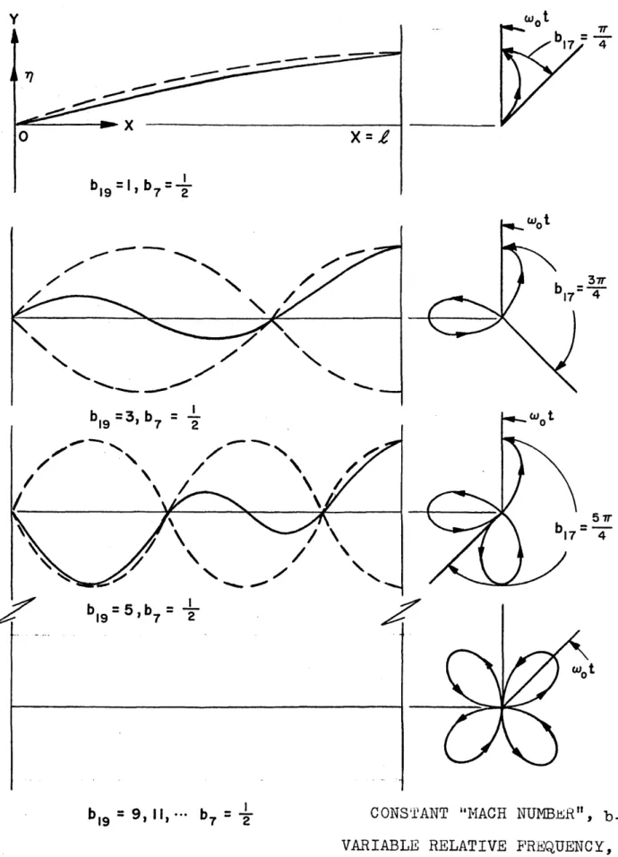
(V-9)

The first term ~enresents the amplitude or limiting shane of the mode. ~he second term is the time variation

containing a correction for the phase at different x. This phase correction will be discussed when three-dimensional shapes 81:'econsidered "because b_r7 is actually the angle in the y-z plane th1:'oughwhich the filament path rotates from

The time va1:'iationis such that at each ~ point through which the filament

z

= 0 to ~ = 1

R

~.

between ~

=

0 and ~

=

1, the

passes, oscillates laterally at frequency, 'J.Jo • Por b'9 equal to odd integral values, the amplitude function is a minimum and the shape becomes b~ quarter sine waves with an amplitude of

no.

This is shown in Figure 6, where ho is introduced as

the maximum amplitude of lateral displacement, which for this case is h_o = r_{o •}

If the value of b~ is not an odd integer, the magnitude of h_o increases from its minimum value, roe This is shown in

Figure

7,

a typical resonance diagram. For zero air drag (b~ = bs = 0) the predicted amplitudes can become very large. This is,however, a result of the assumption of linearity.

Figure 7 is more realistic when the energy loss caused by air drag is considered _{(ba ~ 0, bs}

f

0). Under these conditions the maximum amplitude of the system, h_o, is considerably reduced.

The final correction to the k_o solution for b~

=

_bs = 0, relates to the exponential amplitude. Since positive values of b₃ mean an air flow of positive velocity (toward increasing ~) this correction is seen to be a decrease in the amplitude

of oscillation at each ~. The ma~nitude of this correction decreases for increasing ~, until for

t

= 1, there 1s no correction.

y h o

r--::;~~==~

o

lo=

---/,~

bl9

=

I -h_o ~:__---~?---~ b_l9 =3

---~----~-~-~-~~--~-~j

1t---:---1I b₁₉=OO FIG. 6 AMPLITUDE FUNCTION vs X, b₃ = b₅=0

o

FIG. 7

AMPLITUDE FUNCTION vs big J MAXIMUM VALUE

-42-For ra~~4 0, the boundary conditions include harmonic oscillation at ~ = 0, of frequency, bJo~~' and phase angle,.~~

The solution for ; now becomes:

" x (r x ) ( ~(~ -1))

- =

g(R')

l

A

sin(wo t-b,,(l-

i"»

t

e ,.S .

1.. b:s"" x (V -1

u )

+ g~'( 1- ~) ~~a " sin( w:'t+l6+b,"t.:~))

3

l

a2 jl ~

A simnle illustration of the above boundary conditions would be a flexible filament which moves at velocity, v, between two guides which 'move harmonically and are in phase. This represents the type of oscillatory input that a vibrating machine gives to a flexible filament as the filament moves

through guides attached to the machine. To simplify the interpretation, let b,3= b_s

=

0, _ro

=

ro{~= 1, and \JVo=\4)~~.

Equation V-IO becomes:

-'?l sin(t.lJot-b,..,(l-

j)

)sin bt1~ +sin(UJot+9f+bn1)sin(brCl~(1-

i»

~ = - <V-ll)

sin b,'i~

For

%

=

0, an oscillatory translation of the machine is represen~ed, while for

p

=

180°, an oscillatory rotation of the machine is represented. The two plots in Figure 8 show the unper half of the amplitude envelope of the space curves

(Equation V-Il) for ~

=

0 and ~

=

1800_{, and for three odd}

integral values of b~. Again it is mentioned that odd integral values of b\C\yield minimum filament amplitude, while for b,Gt equal to even integers, maximum amplitude occurs, limited by air drag (and energy loss in the filament itself).

-43-SIN W_o t FOR ep = 0 J r0 = r0

*

= I ~- __ ~v

_.~J_-) x=£ SIN W_o t V--l ...-'!€- __ SIN W_ot

=

r_o

*

=

I ---r--~V FIG. 8

TYPICAL MACHINE OSCILLATIONS

-44-. The linear solution or this thesis is ror constant filament tension. The tension is not constant, however, but is a function of filament shape. The first order change

in tension can be found by considering the constant tension solution as being approximately correct and calculating the variation in tension necessary to satisfy conservation of momentum. This can be done as follows:

~

From conservation of momentum in the i-direction;

x= .Jl

~7.~

if guide friction and ~A ~t~ are neglected. By letting TmQ,r. = To + AT, then for small

e,

AT

e~,.

T=-2-a

(V-12)

Since it is also true that for small

e ,

e

=A~/AX,

then it is nossible to differentiate the expression for~(for zero air drag) and solve for AT/Toe This yields:

SUbstituting this expression into Equation

V-12

gives:

i.e. AT T() oT T

=

t (

v1Wprg lr

roo

(a) c(l- ca.)(sinbtq2) =

ty~ ~ .

v"" blor? .

1Tr-

(b) (.1- c.)(sin b,q2)

(V-13)

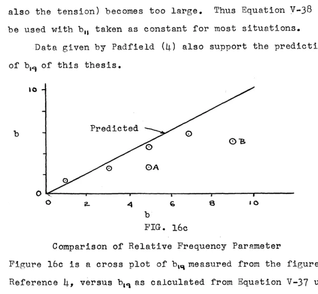
Equation V-13a is of practical importance since it allows the increase in tension to be predicted as a function of the system design variables. It also serves to estimate how good the constant tension assumption is. If the parameter ~ois introduced into Equation V-13a, where b~ois defined as;

2. ::z..

b - 6T _ l (~) ( b'2- )

:LO -

T -

'2" 2b sin h.-:!r

o x 7 -~~

then it is possihle to estimate the limit of the linear solution, since for b~o (~ I, the solution is correct.

Considering again the wave number equation, Equation 1I1-14, a second approximate solution can be obtained. This solution refers to filaments with large bending stiffness, but with small Coriolis' and longitudinal air velocity effects

(small b₁ and b_3). This second solution is outlined as follows.

Note: In fluid mechanics, pressure rises or pressure drops are expressed as functions of the free stream stagnation

_If V;II

pressure, Po- ~. An analogy can be made between this concept and the parameters of Equation V-ljb. In this

AT

equation the filament stress, 1l.' is analogous to the sta~nation ~ressure p.; the filament density is analogous to the fluid density; and the corrected maximum lateral velocity w.ro/(l- ~:)(Sin bA~) is analogous to the free stream velocity,~. Analogies such as this are helpful in appreciating the physical significance of filament parameters.

-46-Let k~ be a root of the wave number equation (Equation 111-14) for b-:L.= b3 =

o.

4 2-Therefore: b l (k~R.)+(k,3i) +(b4+ibr;) = 0 I k₃.l!

=

:!:

t

2~,

1z.. (

:!:

(1-4b• (b.. +ib_s

» ~

-1

J ~

Now let there be one solution of the form:

(V-lq.)

where b «1₃

Substitution into Equation 111-14 yields:

(V-IS)

These four wave numbers are those required for Equation 111-14

for small b~ and b~. They can be wnitten in a more convenient notation' as:'

~here ks refers to Equation

V-IS,

with k₃1 chosen to have the positive sign under the radical and where k_w refers to

Equation

V-IS

with k~R chosen to have the negative sign under the radical.

Using these four wave numbers, ~ks and !k6J a solution can be found which satisfies the boundary conditions of Equations V-I. These conditions (for ro.~~=eo~i-= 0) are:

~-?7($l t) = eo cos wot ~x '

The solution is:

(V-16)

where

DE x (V-I?)

( CDS k Jl + CDS ~Jl) (Si~" ksR ~ - ~ sin k"D x&) ~

= 1 He ( - 5

9. + (sin k

s~n _

1::

~ s ni 17"~x n ) (cos k~gn x - cos k~$n ) DE.

The functions "(.(~)and 4(~(~) require excessive algebraic manipula~ion to be written in any other form. However,

Equations V-lb and V-I? are a complete answer and can be simplified for cases where some of the parameters are zero. For example, let b~

=

b₃

=

b_{s =} 0 (l.e. negligible air drag

and Coriolis' acceleration), then Equation V-lS is reduced to:

(V-18)

For small b, :

This solution is the same as the. k.,2.. solution for b'2.= b₃ =

bs

=

0 and will not be discussed further. For large b_{l :} I +.(h)~ -~ b I

-48-I

Therefore. ~.(! = (~; )"'1- and k ...R. = ik,)! are the .lave numbers to

be used in Equation V-I? to determine the amplitude of the forced response predicted by Equation V-16. This forced

response of filaments of large bending stiffness (with respect to beams) is a well known phenomenon and will not be treated further.

This second approximate solution to Equation II1-14 can be used to obtain an equati.on to predict the natural frequency

of a moving filament,Jl~. This is done as follows for boundary conditions of zero slope and zero displacement at

the guides. These conditions are:

~. '11 '1'{'

o/(O,t) = -(O,t) = -(l,t) = -(l,t)

R ~ ~ ~

The original form of

1

was chosen as:

Equation V-lS, with b~

=

b₃ = b_{s =} 0, is:

Therefore r.tcanbe expressed as:

To fit the above boundary conditions the following equation must be satisfied. (or D₆

=

0).

cos k ~)lcoshks{l

i~

~(t -~

sin ksSlsinh ks.Q

~~=

1 (V-19)