HAL Id: insu-02098484
https://hal-insu.archives-ouvertes.fr/insu-02098484
Submitted on 23 Apr 2019
HAL is a multi-disciplinary open access
archive for the deposit and dissemination of
sci-entific research documents, whether they are
pub-lished or not. The documents may come from
teaching and research institutions in France or
abroad, or from public or private research centers.
L’archive ouverte pluridisciplinaire HAL, est
destinée au dépôt et à la diffusion de documents
scientifiques de niveau recherche, publiés ou non,
émanant des établissements d’enseignement et de
recherche français ou étrangers, des laboratoires
publics ou privés.
Variations of Solar Oblateness with the 22 year-magnetic
Cycle Explain Measurements Apparently Inconsistent
Abdanour Irbah, Redouane Mecheri, Luc Damé, Djelloul Djafer
To cite this version:
Abdanour Irbah, Redouane Mecheri, Luc Damé, Djelloul Djafer. Variations of Solar Oblateness
with the 22 year-magnetic Cycle Explain Measurements Apparently Inconsistent. The Astrophysical
journal letters, Bristol : IOP Publishing, 2019, 875 (2), pp.art. L26. �10.3847/2041-8213/ab16e2�.
�insu-02098484�
Variations of solar oblateness with the 22yr magnetic cycle explain measurements apparently inconsistent
Abdanour Irbah,1Redouane Mecheri,2 Luc Dam´e,1 andDjelloul Djafer3
1LATMOS/IPSL, UVSQ Universit´e Paris-Saclay, Sorbonne Universit´e, CNRS,
11 BD D’Alembert Guyancourt 78280 France
2
Centre de Recherche Astronomie Astrophysique et G´eophysique,
CRAAG Bouzar´eah
16340 Algeria
3Unit´e de Recherche Appliqu´ee en Energies Renouvelables, URAER
Centre de D´eveloppement des Energies Renouvelables, CDER, Gharda¨ıa
47133 Algeria
(Received ... .., 2018; Revised ... .., 2019; Accepted ...) Submitted to ApJ Letters
ABSTRACT
The solar oblateness results from distortion processes due to several phenomena inside the Sun but also induced by the centrifugal potential of the surface rotation. This fundamental parameter is therefore of great scientific interest, but its measurements for more than a century are still very controversial, whether for its average value and/or its variations observed or not over time. Special images acquired for almost the whole Cycle 24 by the Helioseismic and Magnetic Imager (HMI) onboard the Solar Dynamic Observatory (SDO) are used for calculating solar oblateness. The average oblateness obtained is 8.8 ± 0.8 milli-arcseconds in good agreement with measurements of the last two decades. Variations are observed in anti-phase with the solar activity during cycle 24 whereas they were in phase with activity for Cycle 23. More generally, the trend of both in phase variation during odd cycles and anti-phase variation during even cycles is confirmed when revisiting past measurements. Therefore, it is possible that the sun initiates a physical process resulting in a pulsation with the 22yr magnetic cycle having extreme values during the polarity reversals with a maximum swelling during odd cycles and vice versa for even ones. This oscillation could explain the controversy surrounding past measurements.
Keywords: Sun: fundamental parameters — methods: data analysis
1. INTRODUCTION
The internal dynamics of the Sun from its depths to the most superficial layers is manifested by visible disturbances on the surface of the photosphere. They lead directly small deviations from the sphericity of the Sun. The solar shape thus reflects the internal state of the Sun and the processes that take place there. It soon drew the attention of Newcomb (1865), who asked why the Newtonian gravitational theory could not correctly predict the advance of
Mercury perihelion observed byLe Verrier(1859). He suggested that a 500 milli-arcsecond (mas) oblateness i.e. the
pole-equator radius difference, due to a rapidly rotating interior of the Sun could provide an explanation (Newcomb
1895). The solar shape involved two main issues at this stage, namely the theory of gravitation and the internal
rota-tion of the Sun. The advent of Einstein’s theory of General Relativity brought explanarota-tion to the anomalous advance of Mercury perihelion but it remains that good estimates of solar oblateness is of great importance for this theory i.e.
gravitational moments of the Sun is still relevant for the Mercury perihelion (Chapman 2008). Many measurements of
Corresponding author: Abdanour Irbah
2
solar oblateness have been carried out for several decades, bringing other questions about its mean value and temporal variations. A good review on the history of oblateness measurements and the issues they have raised, may be found
in the papers ofDicke & Goldenberg(1974) andRozelot & Damiani(2011). Some scientific events need, however, to
be recalled. The measurement of Dicke and Goldenberg’s solar oblateness in 1966 in Princeton, New Jersey, is worth mentioning because of its high value (41.9 ± 3.3 mas), which allowed them to highlight the scalar-tensor theory of
gravitation and the quadrupole moment of the Sun associated to a rapidly rotating core (Dicke & Goldenberg 1974).
These results were widely criticized but have sparked growing interest in studying the interior of the Sun. Among the
critics, Sturrok & Gilvarry (1967) have shown that a rapid change of internal magnetic field would cause magnetic
distortions at the surface resulting in an oblateness comparable to the observations. The magnetic field then appeared as the third major issue involved in the solar shape. Gravitational models with contribution of helioseismology, which probes Sun’s interior to estimate both radial profiles of latitudinal differential rotation and the internal magnetic field (Goode & Thompson 1992; Antia et al. 2000; Paterno et al. 1996), made it possible to identify acceptable values for oblateness mostly induced by the centrifugal force on surface layers with a very weak contribution from the
grav-itational quadrupole moment J2 (Armstrong & Kuhn 1999; Mecheri et al. 2004; Antia et al. 2008). Measurements
made in space (Fivian et al. 2008;Irbah et al. 2014), on balloons (Egidi et al. 2006) and on ground (Hill & Stebbins
1975;Rozelot et al. 2009) confirmed the expected values. Temporal variations are just as useful for understanding the functioning of the Sun in relation with its activity cycle. Particularly, helioseismic inversion revealed an insignificant
temporal variation of J2 with, in counterpart, variation of surface layers properties (Antia et al. 2008;Lefebvre et al.
2007) correlated with solar cycle, suggesting that shape variations of the Sun are certainly associated with the magnetic
field. Therefore, accurate scrutiny of surface layers of the Sun is very important and requires high precision
helio-seismology for a good resolution of their structure (Reiter et al. 2015). Time series of oblateness recorded on ground,
balloons and lately from space showed variations without, however, being conclusive. They are in phase (Damiani et al.
2011; Rozelot et al. 2009; Dicke et al. 1987; Emilio et al. 2007) or anti-phase (Egidi et al. 2006; Meftah et al. 2016)
with the solar activity but some authors reported no obvious variations (Kuhn et al. 2012) (Fig.1). The longest time
series recorded in space, still in progress, was recorded with the Helioseismic and Magnetic Imager (HMI) onboard the Solar Dynamics Observatory (SDO). SDO was launched on February 2010 just after the beginning of Cycle 24 and the series of HMI measurements now covers almost the whole cycle. These measurements are therefore a major asset to explain and validate those carried out in the past, including explaining reported inconsistencies.
2. HMI DATA AND PROCESSING
Angular variations of the solar shape and their evolution in time are obtained from roll calibrations performed on SDO/HMI twice a year since its launch. This calibration mode consists of rolling the spacecraft around an axis close
to HMI line-of-sight and taking images at constant angular positions during rotation (11.25o
since October 2010). This procedure will later allow removing effects on the solar shape of both mispointing and optical distortion when processing image sequences. Full images of the Sun are recorded in linear polarization at narrow wavelength band
(76 m˚A) in the solar continuum near the Fe I absorption line at 617.3 nm. They have an angular resolution of 1
arc-second. Their size and angular sampling are 4096 x 4096 pixels and 0.5 arc-second, respectively. A complete roll calibration takes about 7 hours while the instrument is subjected to various thermal stresses on its orbit. The method used to process Solar Diameter Imager and Surface Mapper (SODISM) data of the PICARD distortion mode (Irbah et al. 2014) similar to SDO calibration roll, is then applied for HMI image sequences. The processing method
is well detailed inIrbah et al.(2014) and the main steps are recalled. The first step is to extract the solar shapes from
images of the sequence. The position of the inflection point of the Limb Darkening Function (LDF) for all azimuth angles is calculated for this purpose. LDF angular sampling of SDO images is good enough to detect photometric contaminations due to active regions (sunspots, faculae ...). Our used processing method based on wavelet transform preserves LDF inflection point positions defining the solar shape since bad or hard LDF filtering modifies its slope
leading to inflection point shifts (Irbah et al. 1999). Nevertheless, active regions can still affect the mean solar shape
computed from all ones of the sequence previously re-phased in azimuth in order to remove effects of both mispointing and optical distortion during averaging. These contaminations appear when solar active regions are localized very close to LDF inflection points. They are, however, easily detectable thanks to the roll procedure properties and then removed during processing. Indeed, rolling the spacecraft causes the solar image to rotate on the HMI CCD camera. All CCD defaults remain on fixed positions in the frame while solar features move with the spacecraft rotation. The roll sequence recorded on July 22, 2015 is taken to illustrate the main steps of the processing method. Azimuthal
01/01/90 01/01/92 01/01/94 01/01/96 01/01/98 01/01/00 01/01/02 01/01/04 01/01/06 01/01/08 01/01/10 01/01/12 01/01/14 01/01/16 01/01/18 Date 0 5 10 15 20 25
Equator-pole radius difference (milliarcseconds)
0 50 100 150 200 250 Sunspot number RHESSI MDI (SOHO) SDS HMI (SDO) (21) HELIOMETER (PIC DU MIDI) SODISM (PICARD)
Figure 1. Equator-pole radius difference measured with the Heliometer at the Pic du Midi (France), with SDS on balloon and
from Space (RHESSI, MDI, HMI, SODISM) along with sunspot number (SILSO data 2018). The HMI value is the average
over the period 2010-2012 of previous measurements since no variations with solar activity were reported (Kuhn et al. 2012).
SDS measurements exhibit anti-phase variations in the descending phase of Cycle 22. Measurements made with the Heliometer during Cycle 22 have necessarily important error bars since obtained from ground but they still properly overlap SDS ones. Nevertheless their amplitudes prevent to identify a conclusive phase variation with activity. Space and ground measurements made during Cycle 23 are in phase with solar activity. Note that the first Heliometer measurement of Cycle 23 corresponding to solar activity maximum seems underestimated. This value corresponds to the resumption of measurements with the instrument after an interruption of 2 years (1997-1999).
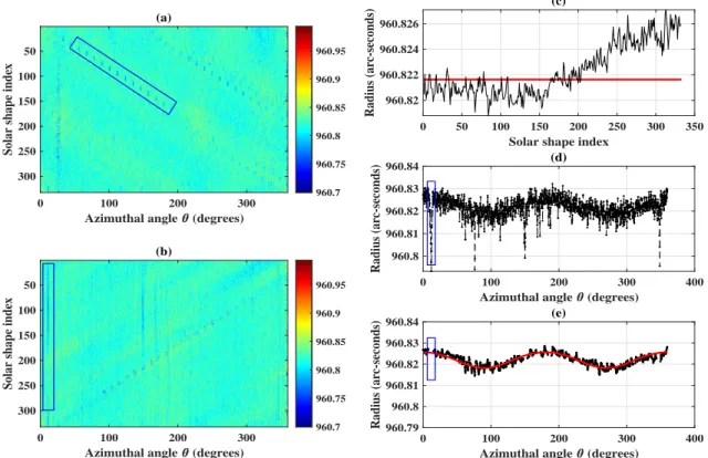
radius variations extracted from all images of the sequence are shown in Figure 2(a). They are coded in a false color
frame where each line is the azimuthal solar radius obtained from one image. Active regions on the extreme solar limb
affect the radius at several azimuthal angles. Some effects are shown within the rectangle in Figure2(a). These effects
move in an oblique direction as the spacecraft rotates. Vertical features are also presents but have clearly optical
signatures since they remain fixed during roll operations. Figure 2(b) shows all azimuthal solar radius in the same
reference frame i.e. the West Equator is the origin of azimuthal angles for all lines. We notice that the solar active
regions surrounded by a rectangle in Figure2(a), are now spread out along the same vertical direction since they are
quasi fixed on the Sun surface. The average radius of each line of the frame varies over time during the roll calibration
(black curve in Fig. 2(c)). It is then corrected with an iterative process to have the mean radius computed over the
entire sequence (red curve in Fig.2(c)). Finally, the solar shape free of both optical distortion and mispointing effects,
is obtained taking the radius mean value for each azimuthal angle (Fig. 2(d)). The angular sampling is 0.2o
. A part of the solar shape affected by active regions on the Sun surface is shown in the region surrounded by a rectangle.
Figure2(e) plots the solar shape where solar active regions were removed and a wavelet transform filtering was applied
to reduce the noise. The solar shape is then fitted using low-order Legendre polynomials (red curve in Fig. 2(e)).
This polynomial fit, up to the fourth order, allows to estimate the quadrupole c2 and the hexadecapole c4 distortion
coefficients. The solar oblateness is then given by ∆R = −3
2c2− 5
8c4 where ∆R is the pole-equator radius difference
or ∆RR = −
3 2C2−
5
8C4 in case of dimensionless C2 and C4; R is the mean solar radius.
3. RESULTS AND DISCUSSION
Sixteen roll sequences, recorded between October 2010 and July 2018, were analyzed according to the processing
4
(a)
0 100 200 300
Azimuthal angle (degrees)
50 100 150 200 250 300
Solar shape index
960.7 960.75 960.8 960.85 960.9 960.95 (b) 0 100 200 300
Azimuthal angle (degrees)
50 100 150 200 250 300
Solar shape index
960.7 960.75 960.8 960.85 960.9 960.95 0 50 100 150 200 250 300 350
Solar shape index
960.82 960.822 960.824 960.826 Radius (arc-seconds) (c) 0 100 200 300 400
Azimuthal angle (degrees)
960.8 960.81 960.82 960.83 960.84 Radius (arc-seconds) (d) 0 100 200 300 400
Azimuthal angle (degrees)
960.79 960.8 960.81 960.82 960.83 960.84 Radius (arc-seconds) (e)
Figure 2. The roll sequence recorded on July 22, 2015 is used to illustrate the processing method. (a) Azimuthal variations of
solar radius obtained from images recorded during the roll. Each frame line coded in false colors corresponds to a solar shape calculated from one image. They are 332 images in this sequence and the number of angular samples is 1800. Some active regions on the Sun (sunspots, faculae ...) as shown by their signature in the rectangle, existed that day and affect the solar shape. (b) Solar shapes are shifted to have all the western equator of the Sun at the zero azimuthal angle. Signatures of active regions affecting the shape are then spread out along frame columns while they are on oblique directions for CCD defaults. (c) A slight time drift of solar radius calculated from each shape (black line) is observed during the roll. It is corrected by mean of an iterative process (red dashed line). (d) All shapes are averaged to compute the mean one where effects of active regions are clearly seen. (e) Active region effects on the solar shape are removed and it is then filtered to reduce the noise. The solar shape is fitted using low-order Legendre polynomials (red curve) to estimate c2 and c4distortion coefficients and, then, the oblateness.
corresponding to a radius difference of 6.4 ± 0.6 km, which is in good agreement with measurements made over the
past two decades (Fivian et al. 2008;Irbah et al. 2014;Egidi et al. 2006;Rozelot et al. 2009). They are also consistent
with values predicted by helioseismology-based models (Armstrong & Kuhn 1999;Mecheri et al. 2004). This average
value is, however, 1.6 mas higher than that reported byKuhn et al.(2012) over the period 2010-2012. In addition to
the coherent values obtained for oblateness, variations in time of the solar shape are of particular importance in view of the scientific controversies of historical measurements. Results obtained show not only that the solar oblateness exhibits variations, but that they are in anti-phase with the sunspot number taken as proxy for activity of the Sun
(Fig. 3(a)). This trend was suspected during the analysis of image sequences taken during the rising phase of solar
cycle 24 (Meftah et al. 2016) and it is confirmed by pursuing it on almost the whole cycle. Kuhn et al.(2012), however,
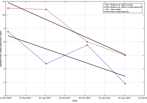
reported no change for the period 2010-2012 using the same SDO data. We calculated solar oblateness from the c2
and c4values of their paper and found a similar temporal trend as we did (see Fig.4). It should be noted that the roll
calibration of January 24, 2018 gives a value of the solar shape that seems underestimated. It is out of the trend that is
emerging, questioning to take it into account or not. The quadrupole C2exhibits variations clearly in phase with solar
activity (Fig.3(b)). Indeed, a linear regression performed between C2 values and sunspot number leads to R2≈ 60%.
We can also mention the yearly variations that seem to appear in the temporal evolution of C2, in particular during
the descent of the cycle of activity. More investigation is needed to find out if these variations are of solar origin or
related to orbital correction residues. Concerning the hexadecapole C4, we notice that it has anti-symmetric variations
01/01/09 01/01/11 01/01/13 01/01/15 01/01/17 01/01/19 Date 6 7.5 9 10.5 12
Equator-Pole radius difference (mas)
(a) 0 40 80 120 160 Sunspot number 01/01/09 01/01/11 01/01/13 01/01/15 01/01/17 01/01/19 Date -8 -7 -6 -5 -4 C2 ×10-6 (b) 0 40 80 120 160 Sunspot number 01/01/09 01/01/11 01/01/13 01/01/15 01/01/17 01/01/19 Date -2 -1 0 1 2 C4 ×10-6 (c) 0 40 80 120 160 Sunspot number
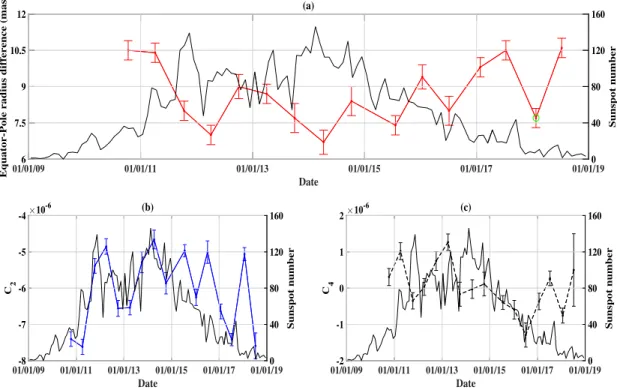
Figure 3. Fit model parameters of equator-pole radius difference obtained from HMI roll calibration images recorded during
Cycle 24. (a) Time variations of solar oblateness (red plot) are clearly in anti-phase with the sunspot number (black line) taken as activity proxy. The value surrounded by green is thought to be underestimated due to poor determination and/or sudden
solar events. The quadrupole variations C2 (blue dots) appear in phase with solar activity (b) whereas the hexadecapole C4
(black dots) has anti-symmetric variations relatively to the time of solar activity maximum where they are very small (c).
of Cycle 24 as already reported by Kuhn et al.(2012) for the period 2010-2012 and in the descent of the cycle but of
opposite sign. This is clearly seen in Fig.5 where we fitted C2 and C4 by sine functions over most of the cycle length.
Rozelot et al. (2009) using C2 and C4 measurements of Emilio et al.(2007), interpreted these temporal variations of
the oblateness by a change of the C4 values that are insignificant when activity is important, but predominant when
activity is low. They suggested that combining both should result in a variation of oblateness in phase with the solar
cycle. We observe the same behavior of C2 than Emilio et al.(2007) but in anti-phase. For C4 we have low values
at the extrema (minimum and maximum) of activity and the variations developing with changing activity (rise and
fall). We indeed have a series of measurements that allow to understand the variation of C4 whereas it is difficult to
evidence a behavior withEmilio et al.(2007) since there are only 2 measurements (1997 and 2001), of which one has
a large error (0.3 +/- 2.5) however consistent with our measurements at high activity. We can see in Fig.3(c) that C4
can vary rapidly in a short period of time, which could explain the difference withEmilio et al.(2007) measurement
obtained in low solar activity (1997). We can conclude from our results that the solar shape is conditioned by both
C2or C4 where the first one evolves in phase with solar activity and the second (C4) varies in phase quadrature with
respect to the other. It is worth also to compare their action on the solar shape with that of a2and a4, even asphericity
coefficients deduced from helioseismology. A recent investigation using both MDI/SOHO and HMI/SDO helioseismic
data over 21 years revealed that during solar activity minimum the asphericity of the Sun is dominated by a2 and
a4 splitting coefficients while during solar activity maximum the a2 coefficient, which primarily describes the solar
oblateness, decreases considerably (Kosovichev & Rozelot 2018). This result indicates an anti-phase variation of the
oblateness with solar activity during Cycle 24 which is in agreement with our results.
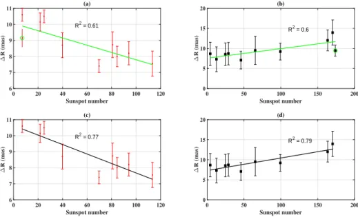
Linear regressions are performed on oblateness versus sunspot number considering all measurements performed during
Cycle 24 (Fig. 6(a)). The negative slope confirms the anti-phase of oblateness variations with the solar cycle. The
linear regression R2
is 61% when all HMI measurements are taken into account and it increases up to 77% (Fig.6(c))
6
01-Oct-2010 01-Jan-2011 01-Apr-2011 01-Jul-2011 01-Oct-2011 01-Jan-2012 01-Apr-2012 01-Jul-2012 Date 4 5 6 7 8 9 10 11
Equator-Pole radius difference (mas)
Kuhn et al. (2012) results Kuhn et al. (2012)'s results linear fit Our results
Our results linear fit
Figure 4. The same temporal trend of solar oblateness exists inKuhn et al.(2012)’s results similar to ours.
all oblateness measurements made during Cycle 23 with the Heliometer (Damiani et al. 2011), RHESSI (Fivian et al.
2008) and SOHO/MDI (Emilio et al. 2007). The linear regression shows a positive slope with R2
= 60%, reflecting
oblateness variations in phase with solar activity during Cycle 23 (Fig. 6(b)). The first measurement made in 2000
with the Heliometer seems, however, underestimated. This corresponds to the resumption of measurements after a
2yr interruption. The linear regression R2
increases up to 79% when this value is removed (Fig.6(d)). Oblateness
measurements performed on balloons with the Solar Disk Sextant (SDS) in the descent of Cycle 22 are in anti-phase with the activity confirming the temporal oscillation of this solar parameter. Taken from ground, measurements with
01/01/2010 01/01/2012 01/01/2014 01/01/2016 01/01/2018 01/01/2020 Date -8 -7.5 -7 -6.5 -6 -5.5 -5 -4.5 -4 C2 10-6 (a) 01/01/2010 01/01/2012 01/01/2014 01/01/2016 01/01/2018 01/01/2020 Date -2 -1.5 -1 -0.5 0 0.5 1 1.5 C4 10-6 (b)
Figure 5. C2 (a) and C4 (b) temporal trends fitted with sine functions (red full lines) showing how they evolve during solar
0 50 100 150 200 Sunspot number 0 5 10 15 20 ∆ R (mas) (b) R2 = 0.6 0 50 100 150 200 Sunspot number 0 5 10 15 20 ∆ R (mas) (d) R2 = 0.79 0 20 40 60 80 100 120 Sunspot number 6 7 8 9 10 11 ∆ R (mas) (c) R2 = 0.77 0 20 40 60 80 100 120 Sunspot number 6 7 8 9 10 11 ∆ R (mas) (a) R2 = 0.61
Figure 6. (a) All measurements of equator-pole radius difference made during Cycle 24 are plotted versus sunspot number
taken as proxy for solar activity. The linear regression performed on these 2 solar parameters is good giving R2= 61% (green
line). (c) The linear regression is better with R2
= 77% (black line) when the perturbed HMI measurement shown in Fig.3(a)
by a dot surrounded with a green circle is not taken into account. The negative slope shows, as expected, that oblateness variations are in anti-phase with solar activity. (b) Same plot as in (a) when all measurements recorded during Cycle 23 are
considered. The linear regression shows a positive slope with R2
= 60% expressing that oblateness variations are in phase with
solar activity during Cycle 23 (green line). (d) A better linear regression is obtained with R2
= 79% (black line) when the supposed underestimated value recorded with the Heliometer in 2000 is not taken into account.
the Heliometer made during the same period have naturally a limited precision and larger error bars, but properly overlap those of SDS (Fig. 1), bringing more confidence in their value. Both SDS and the Heliometer had the merit to allow advance in the knowledge of the temporal variability at a time period when very few data were available. It is also worth noting Poor’s analysis (1905) of earlier oblateness measurements made during Cycles 11 and 13, as
well as Ambronn and Schur ones (1905) made during Cycles 11 and 12 (see Fig. 1 inDamiani et al. (2011)). Despite
the limited precision of these historical measurements, variations although very large, are clearly in phase with solar activity of Cycles 11 and 13 whereas, during Cycle 12, they are very similar to HMI variations observed around the maximum of solar activity, that is to say in anti-phase. Accordingly, it is possible that the Sun initiates a physical process that results in a pulsation with a period of twice the 11yr solar cycle. It has maximum swelling during odd cycles and vice versa for even ones, i.e. the solar shape oscillates like the magnetic field having extreme values during its polarity inversion. It is therefore the time of the measurements, with respect to the temporal oscillation of solar oblateness, that largely explains the controversy surrounding past measurements reported in the literature. Why oblateness oscillates with the 22yr magnetic cycle of the Sun is another challenge to model, which could probably be addressed by precise diagnostics of surface layers structure and dynamics. The complex structure of the leptocline, as
defined inReiter et al.(2015), is certainly a key to understand the described mechanism.
REFERENCES Antia, H. M., Chitre, S. M. & Thompson, M. J.: 2000,
Astron. Astrophys, 360, 335
Antia, H. M., Chitre, S. M. & Gough, D. O.: 2008, Astron. Astrophys, 477, 2, 657
Armstrong, J. & Kuhn, J. R.: 1999, Apj, 525, 1, 533 Chapman, R.: 2008, Science, 322, 535
Damiani, C., Rozelot, J.P., Lefebvre, S., Kilcik, A. & Kosovichev, A.G.: 2011, JASTP, Issue 2-3, 241
Dicke, R. H. & Goldenberg, H. M.: 1974, ApJ Supp. Series, 241, 24, 131
Dicke, R. H., Kuhn, J. R. & Libbrecht, K. G.: 1987, ApJ, 318, 451
8
Egidi, R., Caccin, B., Sofia, S. et al.: 2006, Sol. Phys., 235, 410
Emilio, M., Bush, R.I., Kuhn, J., Sherrer, P.: 2007, ApJ, 660, L161
Fivian, M., Hudson, H., Lin, R., Zahid, H.: 2008, Science, 322, 560
Goode, P. R. & Thompson, M. J.: 1992, ApJ, 395, 307 Hill, H.A. & Stebbins, R.T.: 1975, ApJ, 200, 471
Irbah, A., Meftah, M., Hauchecorne, A., Djafer, D. et al.: 2014, ApJ, 785, 89
Irbah, A.; Bouzaria, M., Lakhal, L., Moussaoui, R. et al.: 1999, Sol. Phys., 185, 2, 255
Kuhn, J.R., Bush, R., Emilio, E., Scholl, I.F.: 2012, Science, 337, 1638
Kosovichev, A.G. & Rozelot, J.P.: 2018, JASTP, 176, 21 Lefebvre, S., Rozelot, J. P. & Kosovichev A. G.: 2007,
ASR, 40, 7, 1000
Le Verrier, U. J.: 1859, Ann. Obs. Paris, 5, 1
Mecheri, R., Abdelatif, T., Irbah, A., Provost, J., Berthomieu, G.: 2004, Sol. Phys., 222, 2, 191 Newcomb, S.: 1865, Constants of astronomy, US GPO,
Washington, DC, 111
Newcomb, S.: 1895, The Elements of the Four Inner Planets, Bulletin Astronomique, Serie I, 13, 26 Meftah, M., Hauchecorne, A., Bush, R.I. & Irbah, A.:
2016, ASR, 58, 7, 1425
Paterno, L., Sofia, S. & Di Mauro, M. P.: 1996, Astron. Astrophys, 314, 940
Reiter, J., Rhodes, E. J., Jr., Kosovichev, A. G., Schou, J. et al.: 2015, ApJ, 803, 2, 92
Rozelot, J.P. & Damiani, C.: 2011, Eur. Phys.J. H, 36, 407 Rozelot, J.P., Damiani, C. & Pireaux S.: 2009, ApJ, 703,
1791
SILSO data/image, Royal Observatory of Belgium, Brussels