HAL Id: hal-00317554
https://hal.archives-ouvertes.fr/hal-00317554
Submitted on 28 Feb 2005
HAL is a multi-disciplinary open access
archive for the deposit and dissemination of
sci-entific research documents, whether they are
pub-lished or not. The documents may come from
teaching and research institutions in France or
abroad, or from public or private research centers.
L’archive ouverte pluridisciplinaire HAL, est
destinée au dépôt et à la diffusion de documents
scientifiques de niveau recherche, publiés ou non,
émanant des établissements d’enseignement et de
recherche français ou étrangers, des laboratoires
publics ou privés.
Dynamics of Alfvén waves in the night-side ionospheric
Alfvén resonator at mid-latitudes
V. V. Alpatov, M. G. Deminov, D. S. Faermark, I. A. Grebnev, M. J. Kosch
To cite this version:
V. V. Alpatov, M. G. Deminov, D. S. Faermark, I. A. Grebnev, M. J. Kosch. Dynamics of Alfvén
waves in the night-side ionospheric Alfvén resonator at mid-latitudes. Annales Geophysicae, European
Geosciences Union, 2005, 23 (2), pp.499-507. �hal-00317554�
Annales Geophysicae (2005) 23: 499–507 SRef-ID: 1432-0576/ag/2005-23-499 © European Geosciences Union 2005
Annales
Geophysicae
Dynamics of Alfv´en waves in the night-side ionospheric Alfv´en
resonator at mid-latitudes
V. V. Alpatov1, M. G. Deminov2, D. S. Faermark1, I. A. Grebnev1, and M. J. Kosch3 1Institute of Applied Geophysics, Rostokinskaya st., 9, Moscow, 129128, Russia
2Institute of Terrestrial Magnetism, Ionosphere and Radio Wave Propagation, RAS, Troitsk, Moscow region, 142190, Russia 3Department of Communication Systems, Lancaster University, LA1 4YR Lancaster, United Kingdom
Received: 11 October 2002 – Revised: 28 September 2004 – Accepted: 9 November 2004 – Published: 28 February 2005
Abstract. A numerical solution of the problem on dynamics
of shear-mode Alfv´en waves in the ionospheric Alfv´en res-onator (IAR) region at middle latitudes at nighttime is pre-sented for a case when a source emits a single pulse of dura-tion τ into the resonator region. It is obtained that a part of the pulse energy is trapped by the IAR. As a result, there oc-cur Alfv´en waves trapped by the resonator which are being damped. It is established that the amplitude of the trapped waves depends essentially on the emitted pulse duration τ and it is maximum at τ =(3/4)T , where T is the IAR funda-mental period. The maximum amplitude of these waves does not exceed 30% of the initial pulse even under optimum con-ditions. Relatively low efficiency of trapping the shear-mode Alfv´en waves is caused by a difference between the optimum duration of the pulse and the fundamental period of the res-onator. The period of oscillations of the trapped waves is approximately equal to T , irrespective of the pulse duration
τ. The characteristic time of damping of the trapped waves
τdec is proportional to T , therefore the resonator Q-factor
for such waves is independent of T . For a periodic source the amplitude-frequency characteristic of the IAR has a lo-cal minimum at the frequency π /ω=(3/4)T , and the waves of such frequency do not accumulate energy in the resonator re-gion. At the fundamental frequency ω=2π /T the amplitude of the waves coming from the periodic source can be ampli-fied in the resonator region by more than 50%. This alone is a basic difference between efficiencies of pulse and periodic sources of Alfv´en waves. Explicit dependences of the IAR characteristics (T , τdec, Q-factor and eigenfrequencies) on
the altitudinal distribution of Alfv´en velocity are presented which are analytical approximations of numerical results.
Key words. Ionosphere (Mid-latitude ionosphere, Wave
propagation, Modeling and forecasting) – Magnetospheric physics (MHD waves and instabilities, Magnetosphere-ionosphere interactions)
Correspondence to: D. S. Faermark (mostfaer@mtu-net.ru)
1 Introduction
Shear-mode Alfv´en waves in the ionosphere in the frequency range 0.1 to 10 Hz can be reflected from regions above and below the F2-layer maximum because of large (relative to the wave length in the medium) gradients of the refractive index (Polyakov and Rapoport, 1981; Belyaev et al., 1990). The occurrence of such reflections and the absence of a group velocity transverse to the geomagnetic field implies that the resonator for shear-mode Alfv´en waves – the iono-spheric Alfv´en resonator (IAR) – should exist (Polyakov and Rapoport, 1981).
The IAR has been identified in the ground-based observa-tions both at middle (Belyaev et al., 1990, 2000) and high (Belyaev et al., 1999) latitudes. Analysis of Freja satel-lite data (e.g. Grzesiak, 2000) also confirms the existence of this phenomenon in the topside ionosphere. The IAR properties have been studied theoretically by Polyakov and Rapoport (1981); Trakhtengertz and Feldstein (1984, 1991); Lysak (1986, 1988, 1991); Belyaev et al. (1990); Demekhov et al. (2000); Pokhotelov et al. (2000, 2001) and Prikner et al. (2000).
The first numerical model that fully resolved the vertical ionospheric structure has been presented by Lysak (1997, 1999). While previous models studied the response of the ionosphere to waves at a fixed frequency, this model was the first that allowed one to investigate the effects in the iono-sphere under action of a field-aligned current pulse with ar-bitrary time dependence generated by a source of this current in the magnetosphere.
In this paper a numerical model of similar type is used but with another position of the source and a number of simplifi-cations specified by the statement of the problem. The main objective of this work is to analyse features of trapping by the ionospheric resonator of a single pulse of a shear-mode Alfv´en wave for the case when the energy losses of the wave at the E-layer heights are insignificant. This corresponds to night-time conditions at middle latitudes which according to observation data, the IAR Q-factor is relatively high (Belyaev et al., 2000). The E-layer is optically thin at frequencies
500 V. V. Alpatov et al.: Dynamics of Alfv´en waves lower than 5 to 10 Hz for these geophysical conditions, and
it allows us to use integrated conductivity of the ionosphere. Besides, low losses of energy of shear-mode Alfv´en waves at the E-layer heights allow us to neglect the connection of these waves with isotropic fast compressional waves. This connection was the focus of Lysak’s (1997, 1999) results. Therefore, Lysak’s (1997, 1999) model is two-dimensional while our model is one-dimensional. Note that a single pulse of Alfv´en wave is generated at an artificial action (chemical release experiment or rocket exhaust gases) in the ionosphere (see, e.g. Marklund et al., 1987; Gaidukov et al., 1993; Demi-nov et al., 2001). Therefore, we put a source of Alfv´en waves inside the resonator, more precisely, at the heights close to the upper border of the E-layer.
The other purpose of this work is to compare character-istics of the Alfv´en waves generated by a pulse source and trapped by the resonator with characteristics of the Alfv´en waves generated by a periodic source and retained by the res-onator. Therefore, two versions of the Alfv´en wave genera-tors – a single pulse and a periodic wave – will be considered below.
2 Formulation of the problem
Propagation of magnetohydrodynamic waves in three regions is taken into account: in the upper ionosphere at the heights
h≥h0≈150 km, where the plasma is magnetized and
iner-tial currents are important; in the E layer of the ionosphere (h0≥h≥hB≈100 km), where ionospheric conductivity
cur-rents are important; and in the electrically neutral atmosphere between hB and the highly conducting surface of the Earth,
where there are no charges and currents if the displacement current is neglected (see, e.g. Nishida, 1978).
It is assumed that background electric fields and currents are absent, i.e. the high-latitudes conditions are not con-sidered. We shall consider only the shear-mode Alfv´en wave, i.e. the effects of transformation of this wave into the isotropic fast compressional wave will be neglected. There-fore, in what follows for brevity the shear-mode Alfv´en wave will be called the Alfv´en wave or simply the wave. The sys-tem of equations for Alfv´en waves in the upper mid-latitude ionosphere is
1/(µ0VA2) · ∂/∂t ∇⊥·E=−∂Jz/∂z, (1) µ0∂Jz/∂t =−∂/∂z∇⊥·E, (2)
where the z axis is directed upwards opposite to the geo-magnetic field (ez=−B0/B0), Jz and ∇⊥·E are the
field-aligned current and divergence of the wave electric field, respectively, the field E is orthogonal to B0, VA is the
Alfv´en velocity, and µ0is the magnetic permeability of free
space. The first equation is deduced from the current conti-nuity condition and from Ohm’s law for collisionless plasma
J⊥=1/(µ0VA2)∂E/∂t (see, e.g. Nishida, 1978). The
sec-ond equation is the consequence of Faraday’s and Amper’s laws. Note that Eqs. (1) and (2) coincide with the equations
of Lysak’s detailed model (1997, 1999), if in Lysak’s equa-tions one neglects collisions, assumes that the cross scale of the wave is not too small, and takes into account that for the Alfv´en wave the following condition is valid:
∇⊥×E=0. (3)
The continuity equation for the current can be written as
∂Jz/∂z+∇⊥·(J⊥+Jext⊥)=0, (4)
where Jext⊥ is the transverse component of extrinsic current which is considered as a source of waves. Taking into ac-count Eq. (3), the continuity equation in the conducting layer can be written as
∂Jz/∂z+∇⊥·(σpE+Jext⊥ )=0, (5)
where σpis the Pedersen conductivity of the ionosphere. For
definiteness, we place the source inside the conducting layer. In Sect. 5 we shall return to this question and show that our conclusions basically do not depend of the source localiza-tion. The conducting layer was assumed to be optically thin, and Eq. (5) was integrated over z from the bottom up to the top border of the conducting layer. Taking into account that at the bottom border of the conducting layer there are no cur-rents, we obtain the boundary condition for the system of Eqs. (1) and (2) at the height h=h0=150 km:
Jz(h0=150 km)=(−6p∇⊥·E−∇⊥· ∫Jext⊥dz)/sin I, (6)
where 6P is the height-integrated Pedersen conductivity of
the ionosphere and I is the magnetic inclination. The bound-ary condition (Eq. 6) is the condition of short circuit of the source current by conductivity currents and the field-aligned current of the wave. It allows us not to consider propagation of the waves at the region below the E-layer.
The processes inside the source are not studied here, there-fore, we put
−∇⊥· ∫Jext⊥ dz=J0F (t ),
where |F (t )|≤1. For this case, the wave is radiated into the region h>h0, and J0is the amplitude of the field-aligned
cur-rent of this wave close to the source, if energy losses of this wave in the E-layer are neglected.
The upper boundary h1 for Eqs. (1) and (2) is located
above the IAR. At this height the condition for radiation of waves along the geomagnetic field into the magnetosphere is specified and the subsequent reflection of waves from the conjugate ionosphere is ignored.
The system of Eqs. (1) and (2) was solved numerically by the method of characteristics (see, e.g. Rozhdestvensky and Yanenko, 1978) in the following variables (Riemannian invariants):
p=∇⊥·E+RJz, q=∇⊥·E−RJz, (7) where R=µ0VA=1/6A, and 6A is the wave conductivity.
Using these variables, the system of Eqs. (1) and (2) takes the characteristic form
V. V. Alpatov et al.: Dynamics of Alfv´en waves 501 where D=0.5 (p−q)∂ln(VA)/∂z. Boundary conditions for
Eq. (8), taking into account Eq. (6), are
p[1+6P/(6Asin I )]−
q[1−6P/(6Asin I )]=2J0F (t )/6Afor h=h0, (9a)
q=0 for h=h1. (9b)
From Eq. (8) it is seen that the wave p propagates only upwards, and q only downwards. The boundary condition (Eq. 9b) is the condition for radiation of the whole wave up-wards into the magnetosphere at the upper boundary, so that no part of this wave is reflected downwards. Equations (7) to (9) are the formulation of the problem. Note that the waves
pand q are always present simultaneously in a non-uniform medium (∂ln(VA)/∂z6=0), and the term D in Eq. (8) describes
the redistribution of energy between these waves. In this for-mulation of the problem the direction of Pointing vector of the Alfv´en wave coincides with Jz. Therefore in what
fol-lows the main attention will be given to the dynamics of the field-aligned currents in the IAR region.
3 Geophysical conditions
From ground-based observations at middle latitudes it is known that the IAR Q-factor is maximum at night (Belyaev et al., 2000). Figure 1a shows the altitude distribution (along the geomagnetic field) of the Alfv´en wave refractive index
nA=c/VA obtained using the IRI model (Bilitza, 1997) for
medium solar activity – a relative sunspot number W =70, middle latitudes – an L-shell equal to 1.8, in February, at midnight.
The analytical approximation of nA altitude distribution
for the F2-layer, where O+ions dominate, is
nA=nAmexp(0.25(1−x− exp(−x))), x=4(h−hm)/L, (10) where hm is the height of nA maximum for which nA=nAm=c/VAm and L is the characteristic scale of the nA
change with height for h>hm. In the case under
consid-eration nAm=407, hm=345 km, and L=240 km. Note that
qualitatively the relation L=L(O+)=2k(Te+Ti)/m(O+)g is
valid for the F2-layer in the region above the layer maxi-mum. Above the F2-layer, in the protonosphere, where H+ becomes the dominant ion, the characteristic scale of nA
in-creases with height. At the heights where protons domi-nate (N (H+) N (O+)) the scale is given by 1/L=1/L(H+)
=0.5m(H+)g/k(T
e+Ti)+∂ln(B0)/∂z, where B0 is the
geo-magnetic field and ∂ln(B0)/∂z≈−3/(RE+h). The height
where 1/L(H+)=0 corresponds to nA minimum. In our
case this nA minimum is located close to 1300 km, and the
protonosphere is located higher than 700 km.
In what follows, the region near the nAmaximum is called
the central part of the IAR. The upper and lower walls of the IAR are located above and below the central part of the IAR where nAdecreases with distance from this central region. In
the considered case the lower wall of the IAR is very steep and extends to the upper boundary of the E-layer at 150 km.
21
Fig. 1 to the paper by V.V. Alpatov et al. "Dynamics of Alfven waves ..."
100 200 300 400 nA 200 400 600 800 1000 1200 1400 h (km) 0.0 0.4 0.8 Jz/ J0 0.68 -0.2 -0.1 0.0 0.1 0.2 0.3 Jz / J0 (a) (b) (c) 0.9 0.34 1.1 1.3 1.5
Fig. 1. Dependence on height h of: (a) the Alfv´en wave refractive
index nA, (dots are the analytical approximation of nAaccording to
Eq. (10); (b), (c) relative values of the field-aligned current of the Alfv´en waves Jz/J0at fixed points in time. Numerals at the curves are times t in seconds from the turn on of the pulse source. The duration of the pulse is τ =π /ω=0.68 s.
The upper wall is less steep and extends up to ≈1300 km where nA=nAmin=66. In this case the condition (Eq. 9b) for
radiation of the wave into the magnetosphere is specified at the height h=h1=1500 km, i.e. higher than the IAR.
By analogy with analytical studies of the resonator (Polyakov and Rapoport, 1981; Lysak, 1991) we designate the depth of the resonator as ε:
ε=nAmin/nAm. (11)
In the considered case ε=0.16.
In Eq. (6) it was taken that the conducting E-layer is opti-cally thin for the Alfv´en wave of frequency ω. This condition is valid if (see, e.g. Lysak, 1999):
δ=(2/µ0ωσP)1/2 LP,
where δ is the skin-depth, LP is the width of the conductive
layer of the ionosphere, 6P=LPσP. In this case σP=2·10−6
mho/, 6P=0.05 mho, LP=25 km, and the conductive layer is
optically thin for frequencies f =ω/2π 100 Hz. Hence, for the analyzed range of frequencies 0.1 to 10 Hz the condition is valid so long as the conductive layer of the ionosphere is thin.
Note one of the consequences of Eq. (10). For this pur-pose we take into account that at middle latitudes the change in height by dh corresponds to a distance along the geomag-netic field ds=dh/ sin I . If one accepts that Eq. (10) is valid at all heights and sinI does not depend on height, then in-tegration of 2 (nA/c) along the geomagnetic field from the
Earth’s surface up to infinity gives the period of movement of the Alfv´en wave between these boundaries (bounce period):
Tbmax=(1/
√
2) exp(1/4)0(1/4)(L/ sin I )/VAm =3.29(L/ sin I )/VAm,
where 0(1/4) is a Gamma function. In this case Tbmax=1.2 s.
502 V. V. Alpatov et al.: Dynamics of Alfv´en waves 22
Fig. 2 to the paper by V.V. Alpatov et al. "Dynamics of Alfven waves ..."
-0.2 0.0 0.2 0.4 0.6 Jz / J0 0 1 2 3 4 0.0 0.2 0.4 0.6 0.8 τ = 0.68 s. 0 1 2 3 4 Time t (seconds) τ = 2 s. 0 1 2 3 4 0.0 0.2 0.4 τ = 0.2 s. h = 600 km h = 400 km h = 200 km
Fig. 2. Dependence on time t of relative values of the Alfv´en wave
field-aligned current Jz/J0at three fixed heights h for the emitted pulse durations τ =0.2, 0.68, and 2 s. Time is measured from turn on of the pulse source.
integration is located at the height h0=150 km. Integration
between the bottom and top borders of the F2-layer (in this case from 150 up to 700 km) gives Tb=1 s. It is seen that
the Tbvalue does not strongly differ from Tbmaxand the
dif-ference between them is near 20%. It allows us to assume that Tbdependence on the ionosphere parameters is similar
to above Tbmaxdependence on these parameters:
Tb=2.7(L/ sin I )/VAm, b=2π/Tb=2.3(VAm/L)sin I. (12)
Equation (12) can be considered as analytical approxima-tion of numerical soluapproxima-tion of this problem which is applica-ble for the whole really observed range of nAm, L and hm
changes in Eq. (10). Comparison of Tbmaxand Tbshows that
the inaccuracy of such approximation is smaller than 20%. This property of Eq. (10) is used below for the approxima-tion of the IAR eigenfrequencies.
4 Single pulse of the Alfv´en wave
Let the function F (t ) in the boundary condition (9a) be
F (t )=sin(ωt) for 0≤t ≤π/ω; F (t )=0 for t >π/ω, (13) i.e. the source radiates upwards (into the region h>h0)an
Alfv´en wave as a pulse of duration τ =π /ω. The field-aligned current amplitude of this wave near the source is equal to J0if
one neglects the Alfv´en wave energy losses into the E-layer. Below we consider relative changes in the field-aligned cur-rent of the Alfv´en waves Jz/J0in the IAR region.
We put frequency ω=4.6 s−1 (f ≈0.7 Hz) which corre-sponds to the pulse duration of the emitted Alfv´en wave
τ=0.68 s. Figures 1b and c show the altitude distribution of
the field-aligned current of the Alfv´en waves Jz/J0for fixed
times t from the moment the source was switched on. At
t=0.34 s the generated pulse is maximum near the source. At this time just above the source (h≈150 km) the field-aligned current is Jz/J0=0.925, i.e. the energy losses in the E-layer
do not exceed 7 to 8% (see Eq. 9a), and reflection of the waves from the IAR lower wall is almost specular. By the time the source is switched off (t =0.68 s) the pulse maximum reaches the IAR upper wall. At this time Jz>0 in the whole
IAR region. At further propagation of the pulse some part reflects from the IAR upper wall and then reflects from the lower wall. As a result, a region is formed where Jz<0. At t=0.9 s this region is located below approximately 450 km. At t =1.1 s a very wide maximum of the pulse reaches the IAR upper wall. By this time Jz<0 in the whole region of the F2-layer (200≤h≤600 km) and Jz minimum is located
in the central part of this region. This extremum is formed by p and q waves in which Jz<0 (see Eq. 7). The q wave is the wave reflected from the upper wall of the resonator and after that it reaches Jzminimum. The p wave is
associ-ated with the q waves from previous times where it reached the lower wall of the resonator, then reflected from this wall and reached Jz minimum. At t >1.1 s the p and q waves
continue their movement and, having reflected from the res-onator walls, reach the central part of the resres-onator again. They form Jzmaximum, as at this time Jz>0 in the p and q
waves due to their reflections. In Fig. 1 this maximum is seen at t =1.5 s. These are just the oscillations of the Alfv´en waves between the resonator upper and lower walls, i.e. the waves trapped by the resonator. The frequency of these oscillations is ≈6.9 s−1.
It was noted above that reflections of the waves from the IAR lower wall are almost specular and the energy losses in the E-layer are insignificant. The energy losses through ra-diation to the magnetosphere are important. This is evident from the sharp decrease in Jz/J0 at the heights h>800 km
at transition from t=1.1 to t =1.3 s when the main maximum of the Alfv´en wave pulse crosses the IAR upper boundary. Therefore, most of the energy of the waves trapped by the resonator is concentrated close to the central part of the res-onator, i.e. at the heights of the F2-layer. This is evident from Fig 2, where Jz/J0dependences on time at three fixed
heights are shown for different durations of the emitted pulse of the Alfv´en wave. Secondary maxima of Jz/J0 are most
distinct near the IAR central part at the height h=400 km, but they are much weaker at h=600 km and practically absent at
h=200 km. At the height of 400 km the intervals between maxima, beginning with the second maximum (for a short pulse, with the third one), almost do not depend on the emit-ted pulse duration: T =0.91±0.04 s. The value T ≈0.91 s is the fundamental period of the IAR which corresponds to the fundamental frequency of the resonator ≈6.9 s−1.
The frequency is determined by internal properties of the resonator, i.e. depends only on the altitude distribution of the Alfv´en wave refractive index nAin the resonator region.
V. V. Alpatov et al.: Dynamics of Alfv´en waves 503 Eq. (10), is
≈2.6(c/nAmL)sin I ≈2.6(VAm/L)sin I. (14)
The fact that most of the wave energy trapped by the res-onator is concentrated at the F2-layer heights was taken into account in deducing Eq. (14). Therefore, dependence on the ionosphere parameters is similar to the one for b(see
Eq. 12). Calculations show that for night hours at middle lat-itudes Eq. (14) is valid for any level of solar activity and for any season with a deviation of less than 15 to 20%.
If approximation (Eq. 10) is used, the IAR fundamen-tal period corresponds approximately to the double time of the Alfv´en wave propagation from 200 up to 600–650 km. Hence, almost the whole F2 region participates in the for-mation of the trapped waves. Height h∗≈hm+L/4≈400 km
corresponds to the half time of the wave propagation at the distance from 200 to 650 km. This height corresponds to the area of peak values of Jz/J0in the trapped waves, as
super-position of the waves reflected from the top and bottom walls of the resonator occurs in this area (see Figs. 1 and 2). The distance from 200 km up to hmis half the interval from hm
up to 650 km, and for qualitative estimations one can take the characteristic scale of nAchange in the region of the
res-onator bottom wall to be equal to 0.5L.
The waves trapped by the resonator are damped out (see Fig. 2). Their characteristic damping time τdeccan be found
from the ratio of Jz/J0maxima in the central part of the
res-onator, beginning with the second maximum, i.e. the ratio of the second maximum to the third one, etc. In the considered case τdec/T ≈0.95±0.1 irrespective of the emitted pulse
du-ration. Additional calculations at fixed T show that τdec∼1/ε
for the case when energy losses of the waves in the E-layer can be neglected. Similar dependence of τdecon ε also
fol-lows from the analytical solution of the problem for a peri-odic source (Belyaev et al., 1990). Therefore, approximately
τdec=(0.15/ε)T =(0.15/ε)2π/ . (15)
Calculations for mid-latitude winter conditions at near-midnight hours at low, middle and high solar activity show that the inaccuracy of approximation (Eq. 15) does not ex-ceed 10 to 15%. Nevertheless, it should be noted once more that this approximation is applicable only for a case when energy losses of the waves in the E-layer can be neglected.
The resonator Q-factor is usually calculated as a ratio of the real part of the resonator eigenfrequency ω∗to its imag-inary part: Q=0.5 Re (ω∗)/I m(ω∗). In the considered case Re(ω*)=, I m(ω∗)=1/τdecfor the trapped waves, and it
fol-lows from Eq. (15) that the IAR Q-factor for these waves is
Q≈0.5/ε. (16)
For the reasons noted above this equation is valid only for a version when energy losses of the waves in the E layer can be neglected.
The amplitude of the trapped waves (Jz/J0)maxdepends on
the duration of the emitted pulse π /ω. Here (Jz/J0)maxhas its
23
Fig. 3 to the paper by V.V. Alpatov et al. "Dynamics of Alfven waves ..."
0.1 0.2 1 2 3 4 5 ω / Ω 1 1.2 1.4 1.6 ( Jz / J0 )max (a) (b)
Fig. 3. Amplitude-frequency characteristics of the resonator for a
single pulse (a) and a periodic wave after a stationary state has been attained (b). (Jz/J0)maxis the maximum of the relative value of the Alfv´en wave field-aligned current in the resonator region, ω is the wave frequency, is the IAR fundamental frequency.
greatest value at the second maximum of Jz/J0in the height
interval 200 to 650 km. This amplitude is maximum when
ω=ωR≈/1.5. (17)
The frequency ωR corresponds to the pulse duration τR=π/ωR, and from Eq. (17) it follows that the amplitude
of the waves trapped by the resonator is maximaum at the emitted pulse duration
τ =τR≈(3/4)T .
We name ωRas the optimum frequency of the emitted pulse.
It is seen that this frequency is smaller than the resonator fun-damental frequency . It is caused by the fact that (Jz/J0)max
is formed as a result of superposition of the waves reflected from the resonator bottom and top walls which have been formed by one pulse of the wave emitted upwards. The wave reflected from the resonator bottom wall passes twice to the IAR central part, more precisely, to the height h∗≈400 km:
it is reflected from the lower part of the top wall and then is reflected once more from the bottom wall. The wave re-flected from the upper part of the resonator top wall passes once to h∗. The numerical coefficient 1.5 in Eq. (17) cor-responds to optimum conditions when the times of passage of these waves are in agreement between themselves. Note that the characteristics of the Alfv´en wave shown in Fig. 1 correspond to the optimum duration of the emitted pulse
504 V. V. Alpatov et al.: Dynamics of Alfv´en waves
Table 1. Parameters of maxima at the amplitude-frequency characteristic of the resonator for a periodic source obtained from the numerical
solution of the problem and from approximation of the resonant frequencies by Eq. (19) (ωn/)ap.
N 1 2 3 4 5 6 7 8 9
ωn/ 1.00 1.69 2.33 2.94 3.55 4.06 4.61 5.19 5.79
(Jz/J0)max 1.63 1.37 1.31 1.42 1.53 1.60 1.67 1.68 1.70
(ωn/)ap 1.00 1.66 2.30 2.92 3.52 4.11 4.68 5.23 5.76
24
Fig. 4 to the paper by V.V. Alpatov et al. "Dynamics of Alfven waves ..."
2
4
6
8
t
/
T
-1
0
1
J
z/
J
0Fig. 4. Dependence of Jz/J0on time t at the fixed height 400 km for the periodic source with the frequency ω==2π /T , where T is the IAR fundamental period.
Dependence of (Jz/J0)max on the emitted pulse duration
is shown in Fig. 3a more evidently. A clear main maxi-mum (Jz/J0)max=0.235 is seen in it which corresponds to
the frequency ωR=/1.5. At a lower frequency ω/≈0.2
an additional maximum is seen where (Jz/J0)max=0.192.
For ω/<0.2 the amplitude of the trapped waves decreases quickly with decreasing frequency, despite the increase of time integrated energy in the pulse emitted by the source. The frequency of the waves trapped by the resonator is close to . These waves are generated by a pulse from the source, and each of the trapped waves is damped out. If the frequency is ω , then only the waves generated during the last passage of the emitted pulse through the res-onator can be detected as trapped waves separately from this pulse. The characteristic time of this pulse decrease is ap-proximately equal to 1/ω. The trapped waves can be de-tected separately if this time is smaller than the characteristic time of damping of the trapped waves (see Eq. 14), i.e. if 1/ω<2π/ or ω/>1/2π ≈0.16. The low-frequency maxi-mum at ω/≈0.2 corresponds to this condition.
5 Periodic Alfv´en wave
Let function F (t ) in the boundary condition (Eq. 9a) be
F (t )=sin(ωt) for t ≥0, (18) i.e. the source is switched on at time t=0 and radiates a pe-riodic Alfv´en wave. After some time a pepe-riodic process will be established in the resonator region whose amplitude will not vary in time.
The process of a steady-state establishment for ω= is shown in Fig. 4. It is seen that it takes t ≈8T for the solu-tion to come to a steady-state where T =2π /. But even at
t=4T the amplitude of the waves retained by the resonator is not very different from the maximum one: (Jz/J0)max=1.55,
1.62 and 1.63 at t=4T , 8T , and 10T .
Figure 3b shows the amplitude-frequency characteristic of the resonator for the steady-state situation, where (Jz/J0)max
is the greatest value of Jz/J0maximum in the height interval
200 to 800 km. It is seen that for a wide range of frequen-cies (Jz/J0)max>1, i.e. the energy which has come from a
periodic source can be stored by the resonator and exceed the losses due to radiation into the magnetosphere. At the amplitude-frequency characteristic of the resonator a num-ber of maxima can be seen. The frequencies corresponding to these maxima are resonant frequencies.
Table 1 gives the resonant frequencies ωnand (Jz/J0)max
values for the steady-state situation. The approximation of these frequencies for 1≤n<10 is
ωn= h
(n+0.5)/1.5−0.009(n−1)2i. (19) Table 1 shows that the approximation (Eq. 19) is suffi-ciently exact. Note that the contribution of the nonlinear term in Eq. (19) becomes appreciable only at n >5. There-fore, it can be neglected in most cases of practical interest. In Fig. 3b, the most clear (Jz/J0)maxmaximum is seen at the
fundamental resonant frequency ω1=. As the frequency
in-creases, the (Jz/J0)max maxima become less distinct. The
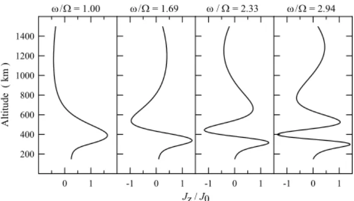
main part of energy of the waves retained by the resonator is concentrated close to the central part of the resonator in the height interval h≈hm±0.25L. It is evident from Fig. 5, that
the dependences of Jz/J0on height are given for the first four
resonant frequencies at fixed points in time when for each of these frequencies the (Jz/J0)maxvalue becomes maximum at
one of these points. In the considered case these maxima are located at the heights 390, 340, 315 and 295 km for the resonant frequencies ω1, ω2, ω3, and ω4, correspondingly.
V. V. Alpatov et al.: Dynamics of Alfv´en waves 505
Table 2. Dependence of the resonator eigenfrequencies on factor K
in Eq. (20). K ω ω2/ ω3/ ω4/ ω5/ 0.6 6.19 1.67 2.30 2.90 3.48 0.8 6.67 1.67 2.28 2.87 3.44 1.0 7.02 1.67 2.27 2.86 3.44 1.2 7.25 1.67 2.27 2.86 3.44 1.4 7.43 1.67 2.27 2.86 3.44
The resonant frequencies ωn are eigenfrequencies of the
resonator. In order to check this conclusion we have in ad-dition solved the problem on eigenvalues when in the initial Eq. (8) the derivative on time is replaced with the complex frequency which was determined from the problem solution. The real values of the resonator eigenfrequencies obtained from this solution differ from the approximation (Eq. 19) by less than 4% for n<10. It implies, in particular, that resonant frequencies will not change if the periodic source is placed in the magnetosphere, under the additional condition that the emitted wave frequency does not change over the wave prop-agation way from the source to the IAR.
Note that if one sets formally n=0.5 in Eq. (19) then the optimum frequency ωR can be obtained for a single pulse
(Eq. 17) when the amplitude of the waves trapped by the resonator is maximum. Nevertheless, the difference be-tween dependences of amplitudes of trapped and retained waves on frequency is essential. For example, Fig. 3 shows that for a periodic source with frequency ω=ωR the
am-plitude of retained waves corresponds to a local minimum ((Jz/J0)max=0.98), i.e. the energy of the waves with this
frequency is not accumulated by the resonator. For a sin-gle pulse of duration τ =π /ωR the amplitude of the trapped
waves is maximum ((Jz/J0)max=0.235). In turn, optimum
conditions for trapping the waves are at a pulse duration which does not correspond to an eigenfrequency of the res-onator, therefore, the amplitude of the waves trapped by the resonator is relatively low even for optimum conditions.
The above estimations were obtained for a specific kind of dependence of the Alfv´en wave refractive index nAon height h(see Eq. 10). In a more general case one can assume that in Eq. (10)
x=4(h−hm)/Lfor h≥hm, x=K4(h−hm)/Lfor h≤hm,(20)
where K is a numerical factor for the IAR bottom wall. The interval 0.6≤K≤1.4 seems to overlap a possible range of K change for typical daytime and nighttime conditions at mid-dle and high latitudes. Analysis showed that for this range of
K change the resonator fundamental frequency depends on K but ωn/ values almost do not depend on K, at least,
for n ≤5. It is seen more evidently from Table 2 where results of the solution of the problem on eigenvalues are shown for the case when for the interval h0≤h≤hmthe approximation
(Eq. 10) is used in which x is described by Eq. (20). For the
25
Fig. 5 to the paper by V.V. Alpatov et al. "Dynamics of Alfven waves ..."
0 1 200 400 600 800 1000 1200 1400 A ltitu de ( km ) ω/Ω = 1.00 -1 0 1 Jz / J0 ω/Ω = 1.69 -1 0 1 ω / Ω = 2.33 -1 0 1 ω/Ω = 2.94
Fig. 5. Altitudinal distributions of relative values of the field-aligned current Jz/J0for four resonant frequencies at fixed points in time t which correspond to Jz/J0maximum in the IAR.
interval hm≤h≤h1the IRI model is used as before. Table 2
shows that in the interval 0.6≤K≤1.4 the fundamental fre-quency changes approximately by 20% and changes in the resonant frequencies ωn/ do not exceed 2%. The difference
between ωn/ values given in Table 2 and the approximation
(Eq. 19) does not exceed 2–3%. It implies that Eq. (19) for
n≤5 is almost universal, i.e. it is applicable for a wide range of geophysical conditions, including day hours. More de-tailed analysis of this property of IAR is beyond the scope of this paper.
6 Discussion
The above stated dependences of and Q on nAaltitude
dis-tribution were obtained on the basis of the analytical approx-imation of the problem numerical solution. Similar depen-dences were obtained on the basis of analytical solution of the problem on eigenvalues with simplifying assumptions of
nAdistribution (Polyakov and Rapoport, 1981; Lysak, 1991,
1999). We compared both results using the above notations and neglecting energy losses of the waves in the E layer. For the version when sin I =1,
n2A=n2Am(ε2+exp(−2(h−hm)/L), h≥hm n2A=n2Am, hm>h≥h0
(21) and εωL/VAm 1 it was obtained (Polyakov and Rapoport,
1981) that the fundamental frequency and Q-factor of the res-onator on this frequency are
=1.25π VAm/(L+1h), Q=(1+1h/L)/(π ε), (22) where 1h=hm−h0. For the above values of hm=345 km, h0=150 km, and L=240 km used we obtain 1h/L=0.81,
=2.2VAm/L, and Q=0.6/ε. It is seen that the analytical
re-sults (Eq. 22) are not strongly different from the numerical ones (Eq. 14) and (Eq. 16). Nevertheless, the altitude dis-tribution (Eq. 21) apparently occurs seldom. In order to ap-proach a realistic situation, another sense should be given to
1hin Eq. (22) – that it is the characteristic altitudinal scale of change of the Alfv´en wave refractive index at the resonator
506 V. V. Alpatov et al.: Dynamics of Alfv´en waves bottom wall. As obtained above for the nA altitudinal
dis-tribution in the form (Eq. 10), its characteristic scale at the resonator bottom wall is approximately equal to 0.5L, i.e.
1h/L=0.5. Substitution of this 1h value into Eq. (22) gives
=2.6VAm/L, Q=0.5/ε, which coincides with Eqs. (14) and
(16) at sin I =1.
For a simpler version when sin I =1, the nA altitude
dis-tribution is described by Eq. (21) with h≥hm, the
bot-tom boundary condition is specified at the height h=hm,
and εωL/VAm 1; Lysak (1991) obtained that
eigenfre-quencies of the resonator are determined by the condition
J0(ωL/VAm)=0, where J0is Bessel function. Recall that the
first five zeroes of J0are 2.40, 5.52, 8.65, 11.79, and 14.93.
Hence, the resonator fundamental frequency is equal to 2.4VAm/L (Lysak, 1991), and
ωn≈[1.305n−0.305], 1ω=ω(n + 1)−ω(n)≈1.305
. (23)
One can see that the fundamental frequency differs weakly from Eq. (14) at sin I =1, but the interval 1ω is approximately twice the interval resulted from Eq. (19):
1ω≈0.67. As an illustrative example, Eq. (19) is written for n=1, 3, 5, i.e. for the first odd values of n:
ω2n−1≈[(2n−1)+0.5]/1.5≈(1.33n−0.33). (24)
The odd eigenfrequencies in Eq. (19) are seen to be very close to those obtained by Lysak (1991). It was noted above that the scale of the resonator bottom wall is approximately equal to 0.5L. Therefore, simultaneous account of the upper and lower parts of the resonator results in the occurrence of additional eigenfrequencies which correspond to even values of n in Eq. (19).
We did not take into account Hall currents, therefore we cannot compare our results with ground-based observations. Nevertheless, we can present here some preliminary estima-tions. For daytime conditions at high latitudes on the basis of the solution of the general problem for a periodic source, Lysak (1999) has obtained that in addition to the fundamental frequency F =f1=0.2 Hz there are two additional maxima:
f2=0.33 Hz and f3=0.5 Hz. Equation (19) can be
rewrit-ten as fn≈F (n+0.5)/1.5. From this equation it follows that f2=0.33 Hz and f3=0.47 Hz, if F =0.2 Hz. It is seen that the
frequencies obtained by Lysak coincide almost exactly with the approximation (Eq. 19). The ground effect of these waves has appeared essentially different: amplitudes of the waves
f1and f3are approximately 3 times as f2amplitude (Lysak,
1999). Therefore, on data of observations in the region of the resonator the interval 1f will be smaller than on the ground-based data (Lysak, 1999).
A similar conclusion can be deduced from data of ground-based observations of the spectral resonance struc-ture (SRS) at middle latitudes (L-shell is approximately equal to 2.65) in winter close to midnight at solar mini-mum. For these conditions the F2-layer critical frequency foF2 ≈2.5 MHz; 1f =1ω/2π ≈2 Hz is the typical value but sometimes 1f ≈1 Hz (Belyaev et al., 1990). This gives
VAm≈870 km/s, sin I ≈0.9. For these conditions L≈210 km,
if the estimations are based on the IRI model (Bilitza, 1997). Substitution of these values into Eqs. (14) and (19) gives the fundamental frequency F =/2π ≈1.5 Hz and
1f ≈F/1.5≈1 Hz. The obtained value is seen to coincide with the minimum 1f interval of observed ones and is ap-proximately half the typical value of 1f ≈2 Hz. Hence, in accordance with Lysak’s (1999) conclusions, ground-based observations show that the even eigenfrequencies of the IAR for the shear-mode Alfv´en waves (f2, f4, ...) are suppressed
and distinguished less clearly than the odd eigenfrequencies. These results show that taking into account the isotropic fast compressional waves is important for analysis of the ground-based data. At the same time the results of analysis by ne-glecting of these waves presented in this paper have allowed us to obtain explicit dependences of characteristics of the shear-mode Alfv´en waves on the distribution of the Alfv´en wave refractive index along the geomagnetic field, and thus have enabled us to compare illustrative data obtained by a number of different ways and under different geophysical conditions.
7 Conclusions
A numerical solution of the problem on the dynamics of Alfv´en waves in the IAR region at middle latitudes at night-time is presented for a case when a source emits a single pulse of Alfv´en waves of duration τ into the resonator region. It was obtained that a part of the pulse energy is trapped by the resonator, i.e. damped Alfv´en waves trapped by the res-onator are formed. It was found that the amplitude of the trapped waves depends essentially on τ and it is maximum at τ =(3/4)T , where T is a fundamental eigenperiod of the resonator. The maximum amplitude of these waves does not exceed 30% of the initial pulse even under optimum condi-tions. Relatively low efficiency of trapping Alfv´en waves is caused by the difference between the optimum duration of the pulse and the resonator fundamental period. The period of oscillations of the trapped waves is approximately equal to T , irrespective of the pulse duration τ . The characteris-tic time of damping of the trapped waves is proportional to
T, therefore the resonator Q-factor for such waves does not depend on T .
The situation changes dramatically when a source emits periodic Alfv´en waves. The amplitude of the waves com-ing from such a source can be increased in the resonator re-gion by more than 50%. This implies that the resonator can accumulate and retain the energy of the Alfv´en waves, de-spite energy losses due to radiation into the magnetosphere. The amplitude of the waves in the IAR is maximum on the resonator eigenfrequencies ωn and this effect is most
pro-nounced when the frequency of the source coincides with the resonator fundamental frequency ω1==2π /T . The interval
between the first adjacent eigenfrequencies of the resonator is 1ω≈/1.5.
For a single pulse the effective frequency ω=π /τ =/1.5 is optimum. For a periodic source the dependence of
am-V. am-V. Alpatov et al.: Dynamics of Alfv´en waves 507 plitude of the retained waves on frequency ω is such that
ω=/1.5 corresponds to a local minimum and the waves of such a frequency do not accumulate energy in the resonator region. This alone is the basic difference between efficien-cies of pulse and periodic sources of the Alfv´en waves.
Explicit dependences of the resonator fundamental fre-quency , harmonics of this frefre-quency ωn, characteristic
time of damping Alfv´en waves trapped by the resonator, and the resonator Q-factor for these waves on altitude distribution of the Alfv´en wave refractive index were obtained. These dependences are analytical approximations of the numerical solution of this problem. These dependences were compared with the ones obtained previously by other methods.
Acknowledgements. This work was supported by the Russian
Foun-dation for Basic Research, project No. 01-05-03890-p98, and Inter-national Science and Technology Center, project No. 1328/99.
Topical Editor T. Pulkkinen thanks a referee for his/her help in evaluating this paper.
References
Belyaev, P. P., Polyakov, S. V., Rapoport, V. O., and Trakhtengerts, V. Yu.: The ionospheric Alfv´en resonator, J. Atmos. Terr. Phys., 52, 781–788, 1990.
Belyaev, P. P., Bosinger, T., Isaev, S. V., and Kangas, J.: First ev-idence at high latitudes for the ionospheric Alfv´en resonator, J. Geophys. Res, 104, 4305–4317, 1999.
Belyaev, P. P., Polyakov, S. V., Ermakov, E. N., and Isaev, S. V.: Solar cycle variations in the ionospheric Alfv´en resonator 1985-1995, J. Atmos. Solar-Terr. Phys., 62, 239–248, 2000.
Bilitza, D.: International Reference Ionosphere – Status 1995/96, Adv. Space Res., 20, 1751–1754, 1997.
Carpenter, D. L. and Anderson, R. R.: An ISEE/Whistler model of equatorial electron density in the magnetosphere, J. Geophys. Res., 97, 1097–1108, 1992.
Demekhov, A. G., Belyaev, P. P., Isaev, S. V., Manninen, J., Tu-runen, T., and Kangas, J.: Modelling the diurnal evolution of the resonance spectral structure of the atmospheric noise back-ground in the Pc1 frequency range, J. Atmos. Solar-Terr. Phys., 62, 257–265, 2000.
Deminov, M. G., Oraevsky, V. N., and Ruzhin, Yu. Ya.: Ionosphere-magnetosphere effects of rockets launched toward high latitudes, Geomagn. Aeron., 41, 738–745, 2001.
Gaidukov, V. M., Deminov, M. G., Dumin, Yu. V., Omelchenko, A. N., Romanovsky, Yu. A., and Feigin, V. M.: “Auroral trigger” experiment, 1. Generation of electric fields and particle fluxes by plasma injection into the ionosphere at high latitudes, Kosmich-eskie Issledovaniya (in Russian), 31, 54–62, 1993.
Grzesiak, M.: Ionospheric Alfv´en resonator as seen by Freja satel-lite, Geophys. Res. Lett., 27, 923–925, 2000.
Lysak, R. L.: Coupling of the dynamic ionosphere to auroral flux tubes, J. Geophys. Res., 91, 7047–7056, 1986.
Lysak, R. L.: Theory of auroral zone PiB pulsation spectra, J. Geo-phys. Res., 93, 5942–5946, 1988.
Lysak, R. L.: Feedback instability of the ionospheric resonant cav-ity, J Geophys. Res., 96, 1553–1568, 1991.
Lysak, R. L.: Propagation of Alfv´en waves through the ionosphere, Phys. Chem. Earth., 22, 757–766, 1997.
Lysak, R. L.: Propagation of Alfv´en waves through the ionosphere: Dependence on ionospheric parameters, J. Geophys. Res., 104, 10 017–10 030, 1999.
Marklund, G., Brenning, N., Holmgren, G., and Haerendelm G.: On transient electric fields observed in chemical release experiments by rockets, J. Geophys. Res., 92, 4590–4600, 1987.
Nishida, A.: Geomagnetic diagnosis of the magnetosphere, Springer-Verlag, N.Y., 1978.
Pokhotelov, O. A., Pokhotelov, D., Streltsov, A., Khruschev, V., and Parrot, M.: Dispersive ionospheric resonator, J. Geophys. Res., 105, 7737–7746, 2000.
Pokhotelov, O. A., Khruschev, V., Parrot, M., Senchenkov, S., and Pavlenko, V. P.: Ionospheric Alfv´en resonator revisited: Feed-back instability, J. Geophys. Res., 106, 25 813–25 824, 2001. Polyakov, S. V. and Rapoport, V. O.: The ionospheric Alfv´en
res-onator, Geomagn. Aeron., 21, 610–614, 1981.
Prikner, K., Mursula, K., Feygin, F. Z., Kangas, J., Kerttula, R., Pikkarainen, T., Pokhotelov, O. A., and Vagner, V.: Non-stationary Alfv´en resonator: vertical profiles of wave character-istics, J. Atmos. Solar-Terr. Phys., 62, 311–322, 2000.
Rozhdestvensky, B. L. and Yanenko, N. N.: Systems of quasilin-ear equations and their application to gas dynamics (in Russian), Nauka Publishing, Moscow, 1978.
Trakhtengertz, V. Y. and Feldstein, A. Y.: Quiet auroral arcs: Ionospheric effect of magnetospheric convection stratification, Planet. Space Sci., 32, 127–134, 1984.
Trakhtengertz, V. Y. and Feldstein A. Y.: Turbulent Alfv´en bound-ary layer in the polar ionosphere 1, Excitation conditions and energetics, J. Geophys. Res., 96, 19 363–19 474, 1991.