Hydrodynamic time parameters response to meteorological and physical forcings: toward a stagnation risk assessment device in coastal areas

HAL Id: hal-02176244

https://hal.archives-ouvertes.fr/hal-02176244

Submitted on 5 Mar 2020

HAL is a multi-disciplinary open access

archive for the deposit and dissemination of sci-entific research documents, whether they are pub-lished or not. The documents may come from teaching and research institutions in France or abroad, or from public or private research centers.

L’archive ouverte pluridisciplinaire HAL, est destinée au dépôt et à la diffusion de documents scientifiques de niveau recherche, publiés ou non, émanant des établissements d’enseignement et de recherche français ou étrangers, des laboratoires publics ou privés.

Hydrodynamic time parameters response to

meteorological and physical forcings: toward a

stagnation risk assessment device in coastal areas

Marion Drouzy, Pascal Douillet, Jean-Michel Fernandez, Christel Pinazo

To cite this version:

Marion Drouzy, Pascal Douillet, Jean-Michel Fernandez, Christel Pinazo. Hydrodynamic time param-eters response to meteorological and physical forcings: toward a stagnation risk assessment device in coastal areas. Ocean Dynamics, Springer Verlag, 2019, 69, pp.967-987. �10.1007/s10236-019-01283-1�. �hal-02176244�

1

Hydrodynamic Time Parameters response to meteorological and physical

forcings: Toward a stagnation risk assessment device in coastal areas

Authors: Drouzy Marion

1,2,

, Douillet Pascal

1

_{, Fernandez Jean-Michel}

2

_{, Pinazo Christel}

1 1_{Aix Marseille Université, CNRS/INSU, Université de Toulon, IRD, Mediterranean Institute of Oceanography (MIO)} UMR110, 13288, Marseille, France

2_{AEL/LEA, IRD Campus, 101 promenade R. Laroque | BP A5 – 98848 Nouméa Cedex, New Caledonia} *ORCID identifier: 0000-0002-3175-2825

Abstract:

Identifying zones of stagnation and deposition of terrigenous matter or contaminants induced by human activity is a key issue in coastal areas. In this paper, circulation processes and potential contaminant stagnation and deposition zones were assessed using hydrodynamic time parameters forced with meteorology. The study focused on an Eulerian time parameter, the local e-flushing time (eFT). The hydrodynamic modeling of coastal zones was applied to two bays of New Caledonia, located downstream of open mining sites. Numerous simulations were performed to classify the influence of forcing conditions on the eFTs variability. The need to consider meteorological forcings rather than average weather conditions for the calculation of eFTs was demonstrated. In coastal zones, high wind velocity was the major forcing influencing eFTs, but below a threshold wind velocity, tidal range and river inputs became significant parameters. Spatial variations of eFTs values, depending on meteorological conditions, induced varying risks of stagnation zones. General responses of the bays’ hydrodynamics and the exposure of zones to potential contaminants were defined under various forcings. Our findings demonstrate that strong turbulence zones are not always characterized by short eFTs because of antagonistic forcing effects. Diurnal tidal alternations were also proven to have less influence on eFT variations than tidal range changes over a lunar cycle.

Keywords:

Residence Time; Coastal hydrodynamic modeling; Meteorological forcings; Mining industry; Stagnation zones; Deposition

Acknowledgements:

This work was partly supported by a CIFRE grant (no. 2015/0175) awarded by the French ANRT (National Association for Technologic Research). The funding scheme was not involved in the study design or submission. The authors would like to warmly thank the whole maritime staff for their support, and laboratory colleagues whose help was truly appreciated.

 Corresponding author: mdrouzy@ael-environnement.nc, AEL/LEA, 101 Promenade R. Laroque, 98800 Nouméa New Caledonia, tel: +687 53 58 68

2

Introduction

The behaviors of shoreline currents, shaping coastal hydrodynamics, determine how particulate and dissolved matter is transported along the coastline. The distance covered by terrigenous matter from its source, for example, depends on local currents (speed, direction, reversals, etc.). Deposition of particles on the seabed is linked to the level of turbulence and size and shape of retention areas. Sediment deposition patterns on the seabed, as well as potential stagnation zones in case of a marine pollution, need to be evaluated for risk assessment policies and can be deduced from knowledge of coastal dynamics. The circulation of currents is controlled by winds, tides, bathymetry and coastline. Field methods are used to understand local hydrodynamics; e.g. lagrangian buoys, ADCP, ADC, and tracking of colored tracer. Whilst being a crucial part of the determination of costal dynamics, their deployment is relatively expensive and numerical models, once validated, provide an effective alternative as they are operational tools designed to investigate the basic mechanisms governing circulation over the continental shelf. Moreover, they allow a spatial and temporal approach to assess water mass movements, facilitating the prediction of dynamics under natural or anthropic forcings.

Hydrodynamics time parameters (HTs) are synthetic indicators allowing a temporal approach to quantifying movements of water masses and matter inside a studied volume (such as a bay, lagoon or enclosed sea). Residence times, or the renewal rate of water masses, are generally used to link hydrodynamics and biomass productivity (Delesalle et al. 1992; Boynton et al. 1995; Bum et al. 1996; Schallenberg & Burns, 1997; Josefson & Rasmussen, 2000). Grifoll et al. (2013) states that a “careful characterization of water renewal is necessary in order to implement a methodology of risk assessment” as HTs provide information on mixing processes (Wolanski, 2008, Cavalcante et al. 2012; Delhez & Deleersnijder, 2012) and can help characterize particle transport and sediment patterns in coastal bays. Conversely, during extreme or intense meteorological events (such as flood or heavy rainfall) water input from river and runoffs, carrying terrigenous matter to the sea, can affect local hydrodynamics to a certain extent (for example a large volume of freshwater discharged into a small bay). Several studies have evaluated water renewal rates by experimental methods (e.g. isotope tracers: Hatje et al. 2017). Our approach used numerical 3D hydrodynamic models to calculate the HTs and relate them to particle transport and sediment dynamics in the Southern Lagoon of New Caledonia. To understand more fully the local hydrodynamics of our studied area, and to highlight the contrast between low and high turbulence zones, the calculation of time parameters were performed to help identify potential deposition zones.

The archipelago of New Caledonia is widely renowned for its coral reef ecosystem, the largest after the Great Barrier Reef of Australia. The marine biodiversity of its lagoon is so rich that it was classified as a UNESCO world heritage site in 2008. In contrast, and despite a worldwide decreasing demand for nickel, open mining and exploitations of nickel form the bedrock of New Caledonia’s economy. This industry relies heavily on the environment, causing deforestation and enhanced erosion; it also increases terrigenous input into the rivers and, eventually, into the lagoon. The fate of these particles or dissolved matter, through transport and deposition, can jeopardize the balance of coastal ecosystems. Corals, for example, can suffer from reduced light penetration or smothering. To assess the risks and prevent damage to fragile marine life, one must firstly understand the transport mechanisms and fate of these terrigenous inputs into the lagoon. This can be done by modeling transport and residence time of a dissolved tracer, acting as a proxy for potential terrigenous dissolved matter, contaminants, or dissolved heavy metals. One of New Caledonia’s current and overriding concerns is ensuring the preservation of the lagoon while managing the impacts of nickel mining on marine ecosystems. Previous studies have been carried out in New Caledonia, investigating large scale HTs over the whole lagoon (Jouon et al. 2006). The present paper aims to focus on smaller scale areas: two bays at the south of the main island (Grande Terre), located downstream of mining sites, and therefore exposed to the influence of the mining industry.

3

The main objective of the study is the characterization of their respective local hydrodynamics, in terms of temporal variables, in order to predict the time needed for a dissolved tracer to be drained out of a control volume of water, subject to physical forcings. This data will help to identify potential risk zones as a function of meteorological conditions.

1. Study Site

New Caledonia (NC) is an island located in the Tropical South West Pacific (TSWP) about 1,500 km off the east coast of Australia, between 20° and 23° south, and 164° and 168° east, as represented on Figure 1. The main island (Grande Terre) is oriented in a southeast to northwest direction. New Caledonia is well known for its coral barrier reef (the largest after the Great Barrier Reef of Australia), which delineates a 23,400 km² lagoon.

The dominant weather features are the migratory subtropical anti-cyclones and southeast trade winds (Salinger, 1995). From its geographical situation, New Caledonia is mainly influenced by two global-scale climatic events, both linked to the South Pacific Convergence Zone (SPCZ) displacement: the Madden Julian Oscillation (MJO) and the El Niño Southern Oscillation (ENSO) (Lefevre et al. 2010). They produce a tropical climate with two main seasons: a wet and warm period during the austral summer (November to March), with steady southeast trade wind episodes (on average 8 m/s), and a dry and cooler period during the austral winter (May to September) when winds are weaker. The inter-seasonal climate is dry and sunny. Inside the lagoon, water flow is mainly generated by tides and local winds (Ouillon et al. 2010). The semi-diurnal tide propagates from south to north (Douillet et al. 1998) and local southeast trade winds drive a general northwest drift (Douillet et al. 2001, Ouillon et al. 2010).

4

Our study sites are two adjacent and sheltered bays located at the south end of the main island (Figure 2). Our study investigates the variability, over time and space, of their physical and sedimentological parameters, through the analysis of their HTs. Port Boisé Bay and Kwe Bay are relatively similar in shape and size, about 2.6 km² and 2.1 km², respectively. Their maximum depths are very comparable and reach up to 40 m (Figure 2). However Kwe Bay deepest values are restricted to the channel, while Port Boisé deep zones span over the main surface of the bay.

Both entrances of the bays are facing southeast. The bays differ for their river inputs. A total of five rivers (incl. Trou Bleu River) and three creeks flow into the bay of Port Boisé, whereas only the Kwe River discharges in the second bay. The average annual flow rates provided by DAVAR (Directorate of Food and Rural Veterinary Affairs) are very low for the creeks (0.06 m3_{/s at medium flow, 0.03m}3_{/s at low flow), and slightly higher for Trou Bleu River (0.2 m}3_{/s at medium} flow, 0.1 m3_{/s at low flow). Kwe River flows in Kwe Bay at a rate of 1.694 m}3_{/s at medium flow, 0.446 m}3_{/s at low flow.} The main difference stands in the exploitation of their respective watershed. Although it used to be exploited in the past, the Port Boisé watershed is no longer under anthropic influence, and we assume that any terrigenous input in the bay is not from human activity. In contrast, the Kwe Bay watershed harbors three open mining sites that are currently exploited. Deforestation and digging along with the mining processes are responsible for soil leaching and transportation of terrigenous particles through runoff. This greatly increases particle transport in the Kwe River and eventually terrigenous inputs into Kwe Bay. These inputs of particles can cause damages to the reef by deposition, shading or smothering of the corals, in addition to the siltation of the river mouth. They also constitute a potential substrate for heavy metals or contaminants inherent to the mining processes.

5

2. Methods

The purpose of using 3D modeling in this study is to assess in details the impact of terrigenous particles inputs, transport and stagnation and under the influence of wind and tide. Indeed, the determination of stagnation zones as a function of meteorological forcing is the first step toward the construction of a proper risk assessment tool. Here we described the model, the parameters chosen and the strategy adopted to meet these objectives.

2.1. 3D hydrodynamic model

A numerical model of circulation and particle transport (MARS3D: Model for Applications at Regional Scale) was adapted to our small-scale study area. The model was originally developed by IFREMER (French Institute for Research and Sea Resource Exploitation) to provide realistic descriptions of coastal phenomena, as described in detail by Lazure and Dumas (2008). Under physical and meteorological forcings such as tide, wind or river inputs, the 3D hydrodynamic model computes the thermodynamic variables of water masses, currents, fluxes, particle transport and deposition, resuspension and concentration of dissolved matter. The governing equations, based on classical assumptions (Boussinesq approximation, assumed hydrodynamic balance), are solved using the calculation of finite differences. The solution of the equation system is divided in two sub-models, one of them being a depth integrated 2D model, solving the shallow water equations (Blumberg & Mellor, 1987) and calculating horizontal velocity and water elevation in every point. Results are then transferred into a 3D model using the same horizontal grid discretized into 30 generalized sigma coordinates on the vertical axis. The interface layers boundary conditions are “slip conditions” with wind stress at the surface layer and friction on the bottom in the deepest layer (Blumberg and Mellor, 1987; Deleersnijder et al. 1992, Torreton et al. 2007). The thickness of the 30 layers varies according to the depth of the mesh considered, following the SCRUM model (Hedström, 2000) and is refined at the surface and bottom of the water column to precisely represent boundary layers.

The spatial and temporal evolution of the concentration of a passive tracer is defined by advection and diffusion terms, same as those for temperature and salinity in the physical model (1):

𝜕𝐶 𝜕𝑡+ 𝑢 𝜕𝐶 𝜕𝑥+ 𝑣 𝜕𝐶 𝜕𝑦+ 𝑤 𝜕𝐶 𝜕𝑧 = 𝜕 𝜕𝑥(𝐾𝑥+ 𝜕𝐶 𝜕𝑥)+ 𝜕 𝜕𝑦(𝐾𝑦+ 𝜕𝐶 𝜕𝑦)+ 𝜕 𝜕𝑧(𝐾𝑧+ 𝜕𝐶 𝜕𝑧)

+ Tend

(1)

Where “C” is the tracer concentration, “u, v, w” are the 3D velocity components of current, “

K

x,

K

y,

K

z” are eddy diffusivity coefficients and “Tend” is the Sources- Sink term.

The turbulence closure is the two equation-scheme known as “k-ε” described by Burchard et al. (1999). The ULTIMATE QUICKEST MACHO multidimensional scheme, a third-order accuracy scheme in time and space (Duhaut and Honnorat, 2008), was implemented for passive tracer advection. Interface zones are very important for optimal description of thermo-physical exchanges between the air and water surface, as well as between near-bottom water and sediment. The interface layers boundary conditions are “slip conditions”, aiming to describe the effect of wind on the water surface; a wind stress condition was applied at the surface (Douillet et al. 2001, Torreton et al. 2007). Bottom stress was parameterized through a quadratic function of velocity representing a logarithmic layer adjacent to the bottom (Blumberg and Mellor, 1987; Deleersnijder et al. 1992; Douillet et al. 1998). Following a sediment characterization cruise, we implemented a spatially variable roughness in the model, according to the type and nature of sediments (silts, sand, corals ...). The heat transport module was not used in the present study, but the simulations reproduced the haline stratification. The 3D model MARS3D was first adapted and validated for the lagoon of New Caledonia in the 90’s (Lazure and Salomon, 1991a,b; Douillet et al. 1998). Since then, the model in

6

its different improved versions has been largely used for hydro-sedimentary studies and compared to measures (Ouillon et al. 2010; Fernandez et al. 2006) and bio-geochemically coupled works (Fuchs et al., 2012; 2013;Faure et al. 2010a,b; Pinazo et al. 2004) with frequent comparisons between model results and in situ data (Plus et al. 2003; Ouillon et al. 2004; Jouon et al. 2006; Ouillon et al. 2005; Douillet et al.2001; Douillet & Legendre, 2008; Fuchs, 2013). In this study, pressure sensors were deployed to record sea level variations, at five sites included in the finest model grid and over a period of 9 months. The pressure measurements, acquired every ten minutes between October 2016 and June 2017, were converted into sea surface elevation (SSE) and compared to the SSE computed by the model for the same period, and forced with tidal currents only. Correlation coefficients between measured and modeled elevations were calculated for each site in order to assess the liability of the model calculations of SSE. To achieve high-resolution modeling of Port Boisé and Kwe bays, three different scales of embedded grids were created using a nesting method. The widest grid, which covers the whole lagoon, has a mesh size of 500 m and is forced by a sea surface elevation (SSE) signal harmonically composed by a TPXO8 model (Egbert et al. 2002) adapted with eleven waves instead of five, in order of importance:

–M2: lunar semi-diurnal – S2: solar semi-diurnal – K1: luni-solar diurnal – O1: lunar diurnal

– N2: lunar semi-diurnal – K2: luni-solar semi-diurnal – P1: solar diurnal – Q1: lunar elliptic diurnal – M4: Shallow water overtides of principal lunar –MN4: Shallow water quarter lunar diurnal

–MS4: Shallow water quarter lunar diurnal sinusoidal

No other boundary conditions were injected into the largest model (neither heat fluxes nor precipitations) as the simulation in this study only aimed at assessing the effect of tidal, wind and river input forcings on HTs. These latter are forced conditions, chosen stationary and homogeneous over the modeled domain so as to distinguish their respective influence on HTs. The intermediate grid is an enlargement of the Southern Lagoon at 180 m resolution. The SSE forcing is taken from the mother grid, before being injected into the finest mesh, covering the bays. The bathymetry of the grids were mapped using various sources, including digitized nautical charts from SHOM (French Oceanographic and Hydrographic Services), previous studies and the bathymetry of the bays mapped using a GPS echo-sounder (see sect. 2.2). The time step was set at 30 s for the 500 m grid, 15 s for the 180 m grid and to 5 s for the highest resolution (60 m) grid. As fine grid resolution leads to better representation of small scale hydrodynamics, an accurate bathymetry was required for the highest resolution mesh grid. A three days cruise was conducted in September 2015 using a GPS echo-sounder in Port Boisé and Kwe bays to acquire bathymetric data (20 m mesh network). The data acquired were then interpolated to fit the 60 m grid model covering Kwe and Port Boisé bays (Figure 2).

2.2. Flushing time definition and computation methods

2.2.1 e-Flushing Time

Numerous definitions of HTs can be found in the literature. They all aim at characterizing local dynamics using temporal parameters but there is no real consensus on which one to use (Grifoll et al. 2013), the choice has to be made regarding of the specificity of each problematic (Monsen et al. 2002) . It is therefore essential to clearly define the variable chosen in this study. The most frequently found HT is the simple ratio between a control volume and the daily fluxes entering and leaving it. It is found in the literature under a diversity of names: “residence times” (Gallagher et al. 1971; Delesalle and Sournia, 1992; Kraines et al. 1998, 1999; Rasmussen and Josefson, 2002; Gomez-Gesteira et al. 2003), “turn over time” (Pagès et al. 2001), “water exchange rate” (Kraines et al. 2001) “water

7

renewal time” (Andrefouët et al. 2001). Another commonly used HT is the time needed for a water parcel at a given point in the volume to exit the volume. This Lagrangian description is referred as “residence time” by Takeoka (1984) and is also found in Du & Shen, (2016), Rynne at al. (2016), it is also called “export time” by Kraines et al. (2001) and “water export time” by Jouon et al. (2006).

An Eulerian approach also exists with the parameter Zimmerman (1976) originally called the “flushing time”. This specific HT is used in this paper and its calculation is based on Thomann and Mueller (1987) definition: Considering a known quantity of a substance in a homogenous water volume at time t0 at an initial concentration C0, with no further amount of this substance is added after t0, with constant fluxes at the water volume boundaries, the concentration of the substance within the water mass at time t is given by the equation:

𝐶(𝑡 − 𝑡

₀

) = 𝐶

₀

𝑒

−𝑄 𝑉∗(𝑡−𝑡⁄ 0)

_{= 𝐶}

0

𝑒

(−

𝑡−𝑡0

𝜃 )

₍₂₎

Where Q represents the flux of substance (entering or exiting), V is the volume of the control volume considered, t is the time and θ is the e-flushing time. Many authors adopted this value also called “residence time” by Rasmussen and Josefson (2002), Wang et al. (2004), Shen and Haas (2004) and Cavalcante et al. (2012); “e-folding time” by Dettmann et al. (2001) and Delhez et al. (2004). Monsen et al. (2002) points out that this concept not only accounts for adjective flux as mechanism of transport but also for additional transport process such as dispersion. However, they emphasize the necessity of defining the underlying assumptions of every this formulation; Thomann and Mueller equation implies a steady flow of the water mass transporting the substance injected, and no addition of substance after t0. Finally the flow and water volume are considered constant over the time of the simulation. On these conditions, “the e-flushing time” is the time after which the tracer concentration initially injected in the control volume is reduced by a factor of 1/e (Weinbauer et al. 2010 ; Thomas et al. 2010; Grifoll et al. 2013; Sanchez-Garrido et al. 2014; Green et al. 2018).

2.2.2 Local e-Flushing Time: local eFTs

The parameters cited above are general parameters, defined for an entire domain or volume, and therefore do not take into account the space and time variability of the hydrodynamics. Cucco et al. (2009) and Delhez et al. (2014) recommend the use of local HTs, defined for each grid point, in impact studies focusing on the persistence of a pollution issue. Grifolls et al. (2013) also used this Eulerian approach “which seems […] more suitable to reproduce water renewal process in tidal active basin”. In the final purpose of tackling issues such as local pollution or particle deposition, we adopted the e-flushing time (eFT) described above and aligned on this designation largely used for tropical lagoon hydrodynamic studies (Torreton et al. 2007; Rochelle-Newall et al. 2010; Fichez et al. 2010; Caravaca et al. 2012). We adapted it to our local scale by computing a hydrodynamic time for each mesh of the grid. To do so, an arbitrary concentration of a conservative dissolved tracer, C0=1, is initially set on the whole domain of interest, and the rest of the grid is set to zero. The evolution of this concentration is calculated over the time of the simulation. Following the methodology of Jouon et al. (2006), when tracer concentration reaches the threshold value C1=95% of C0, an exponential decrease start in the grid element. C1 happens at time t1, which is called the “flushing lag” (Muñoz et al. 2012). The “local e-Flushing Time” is computed for every mesh of the grid using exponential concentration decay between C1 and C0/e. This regression is found to correlate best with the real concentration decrease (Figure 3). It implies the creation of two variables which can vary under the influence of physical forcings: “the flushing lag”, which is the time needed for external water to reach each grid element in sufficient quantity to trigger a decrease in tracer concentration, and the “local e-Flushing Time”, which is the time required for the concentration to decrease from C1 to 37% of the initial C0 through inputs of external water. Plus et al. (2009) and Cerralbo et al. (under review) consider the sum of the two variables and name it the Local Flushing Time, while

8

Cucco et al. (2009) refers to this sum as the “Eulerian Water Transport” and Abdelrhman et al. (2005) as the “Local Residence Time”. In this paper the “flushing lag” is not considered as the “local e-Flushing Time” can be studied in itself and enables the description of hydrodynamics spatial variability as well as the establishment of areas differentiation within the domain of interest, according to physical forcings.

Figure 3: Expression of exponential decrease to calculate the flushing lag (here FL) at C(t)=C0*0.95, and the local eFTs (here LFT) at C(t)=C0/e

2.3. Modeling strategy

2.3.1. Physical forcing conditions

To highlight potential sensitivity of local eFTs to hydrodynamic forcings, the simulations presented in this paper were forced with selected meteorological conditions in order to obtain a complete overview of their influence on the patterns of hydrodynamic transport and deposition. A total of 102 simulations (Table 1) were computed to reproduce a comprehensive array of 8 wind directions. Every one of them was launched after a one month spin-up, with tide being the only forcing, so as to stabilize the model. For every wind direction, we considered two representative river flow rates (low and medium) to simulate the influence of a dry and a wet season, as in Mahanty et al. (2016). Two wind velocities were representative of the region: 5 m/s and 8 m/s (Le Borgne et al. 2010) and every simulation (specific wind and flow conditions) was run three times during a tide cycle of moderate amplitude: the 2nd_{, the 8}th and the 12th _{of July 2013, in order to cover three different tidal periods: Low tidal rate (LTR), Medium tidal range} (MTR) and High tidal range (HTR).

Wind velocity and direction are almost constant. However, a blank noise of 10% of velocity components was implemented (added or retrieved) on both components for every scenario. This blank noise is calculated to avoid any particular surface wave excitation. The wind conditions were then considered spatially homogeneous over the modeled area. River inputs were set to constant over the simulation time, either low or medium flow. These 102 runs provided enough results for the analysis of the local eFTs variability due to wind direction and intensity, and river flow. In order to ascertain whether tide conditions during a pollution incident must be considered, as demonstrated by De Brye et al. (2011), further simulations were undertaken to determine their statistical weight. Following Torreton et al. (2007), twenty-eight identical simulations were run without wind forcing, every twelve hours, for a total period of 14 days, (Table 2) to assess the variability purely due to tidal range variation over half a lunar cycle. Then, twenty-four other “no wind” simulations were run every hour over a whole day to assess the variability of eFTs due to the diurnal tidal cycle (Table 2). The averaged local eFTs and their weighted standard deviation were analyzed in both cases.

9

Table 1: Description of the 102 different scenarios considered for the simulations. R.F: River Flow (low or medium), W.I: Wind Intensity (5 or 8 m/s), T.R: Tidal Range (L: low, M: medium, H: high) North Wind (n=12 runs) North-East Wind (n=12) East Wind (n=12) South-East (Trade) Wind (n=12) South Wind (n=12) South-West Wind (n=12) West Wind (n=12) North-West Wind (n=12) No Wind (n=6)

R.F W.I T.R R.F W.I T.R R.F W.I T.R R.F W.I T.R R.F W.I T.R R.F W.I T.R R.F W.I T.R R.F W.I T.R R.F T.R

Low 5 L Low 5 L Low 5 L Low 5 L Low 5 L Low 5 L Low 5 L Low 5 L Low L Low 5 M Low 5 M Low 5 M Low 5 M Low 5 M Low 5 M Low 5 M Low 5 M Low M Low 5 H Low 5 H Low 5 H Low 5 H Low 5 H Low 5 H Low 5 H Low 5 H Low H Low 8 L Low 8 L Low 8 L Low 8 L Low 8 L Low 8 L Low 8 L Low 8 L

x Low 8 M Low 8 M Low 8 M Low 8 M Low 8 M Low 8 M Low 8 M Low 8 M

low 8 H low 8 H low 8 H low 8 H low 8 H low 8 H low 8 H low 8 H

Med. 5 L Med. 5 L Med. 5 L Med. 5 L Med. 5 L Med. 5 L Med. 5 L Med. 5 L Med. L Med. 5 M Med. 5 M Med. 5 M Med. 5 M Med. 5 M Med. 5 M Med. 5 M Med. 5 M Med. M Med. 5 H Med. 5 H Med. 5 H Med. 5 H Med. 5 H Med. 5 H Med. 5 H Med. 5 H Med. H Med. 8 L Med. 8 L Med. 8 L Med. 8 L Med. 8 L Med. 8 L Med. 8 L Med. 8 L

x Med. 8 M Med. 8 M Med. 8 M Med. 8 M Med. 8 M Med. 8 M Med. 8 M Med. 8 M

Med. 8 H Med. 8 H Med. 8 H Med. 8 H Med. 8 H Med. 8 H Med. 8 H Med. 8 H

Table 2: Starting dates of the 52 complementary simulations for assessment of tidal variabilities influence on HTs

Starting dates of the 24 simulations

launched for assessment of

the tidal cycle influence on HTs 03/07/2013 00:00 03/07/2013 01:00 03/07/2013 02:00 03/07/2013 03:00 03/07/2013 04:00 03/07/2013 05:00 03/07/2013 06:00 03/07/2013 07:00 03/07/2013 08:00 03/07/2013 09:00 03/07/2013 10:00 03/07/2013 11:00 03/07/2013 12:00 03/07/2013 13:00 03/07/2013 14:00 03/07/2013 15:00 03/07/2013 16:00 03/07/2013 17:00 03/07/2013 18:00 03/07/2013 19:00 03/07/2013 20:00 03/07/2013 21:00 03/07/2013 22:00 03/07/2013 23:00 x x x Starting dates of the 28 simulations launched for assessment of

the tidal range influence on HTs

02/07/2013 00:00 02/07/2013 12:00 03/07/2013 00:00 03/07/2013 12:00 04/07/2013 00:00 04/07/2013 12:00 05/07/2013 00:00 05/07/2013 12:00 06/07/2013 00:00

06/07/2013 12:00 07/07/2013 00:00 07/07/2013 12:00 08/07/2013 00:00 08/07/2013 12:00 09/07/2013 00:00 09/07/2013 12:00 10/07/2013 00:00 10/07/2013 12:00

11/07/2013 00:00 11/07/2013 12:00 12/07/2013 00:00 12/07/2013 12:00 13/07/2013 00:00 13/07/2013 12:00 14/07/2013 00:00 14/07/2013 12:00 15/07/2013 00:00

10 2.3.2. Spatial distribution of Local eFTs

We analyzed local eFTs resulting from each simulation, and eFTs averaged over different sets of simulations. Standard deviations were also calculated (eq. 3). They indicate the variability of local eFT values over a given set of simulations, due to changes in physical forcings (wind intensity, river flow, and tidal range).

𝜌

_{𝑖,𝑗,𝑘}

= √

∑ (𝑥𝑁1 𝑛−𝜇𝑛)2

𝑁

(3)

With

𝜌

_{𝑖,𝑗,𝑘} is the standard deviation for mesh “i,j,k”, N is the number of simulations in the set considered,

𝜇

_𝑛 is the averaged eFT in mesh i,j,k for the set of N simulations,

𝑥

_𝑛 is the eFT value in mesh i,j,k for the simulation n. Yet, these standard deviations are relative variables which depend on the order of magnitude of averaged local eFTs. As a consequence, we introduced a weighted variable per mesh grid by dividing the standard deviation by the mean eFT (eq. 4). This weighted standard deviation, here called the “Variation Rate” and expressed “Wσ”, reveals the variability in eFTs values of a zone due to changes in forcings.

𝑊𝜎

𝑖,𝑗,𝑘

=

𝜌𝑖,𝑗,𝑘

𝜇𝑖,𝑗,𝑘

(4)

Comparisons were made between the two bays and between vertical layers, to identify spatial disparities in hydrodynamics and in vertical eFTs distribution. Mapped representations are provided to illustrate these first results and their spatial variability over the two bays. Theses comparisons were followed by a second analysis of the results, where four zones were determined and separately studied in each bay to distinguish different local dynamic behaviors.

2.3.3. Zonal comparison of physical forcing effects

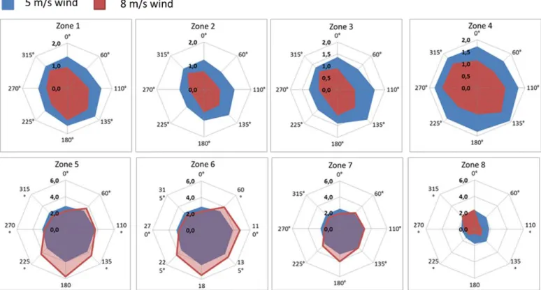
The identification of areas of specific characteristics (differing by their bathymetry or particular location) led to the consideration of eFTs by zone of interest to better characterize spatial variability over the study site. In order to highlight the behavior of eFTs from one area to another, eight zones were distinguished (Figure 2): the river mouths (1, 5 and 6), the channels (2 and 7) and the coral plateaus (3, 4 and 8). The three coral zones are very shallow and delimited by a fringing reef exposed at low tide. The depths of the channels both reach up to 40 m, whereas river mouths do not exceed 1.5 m deep (Figure 2). The results presented by zones were integrated over the 30 sigma levels on the vertical axis, providing eFTs distributions as 2D data. The 8 zones respective responses to changes of wind intensity and direction are presented in the form of radar diagrams, which enable to overlay the different conditions of the simulations.

Results presented in this paper only focus on the HTs within the two bays of interest. The offshore section is not analyzed as this work is part of a bigger study dedicated to the impact of mining industry on the bays.

11

3. Results

3.1. Spatial distribution of Local eFTs

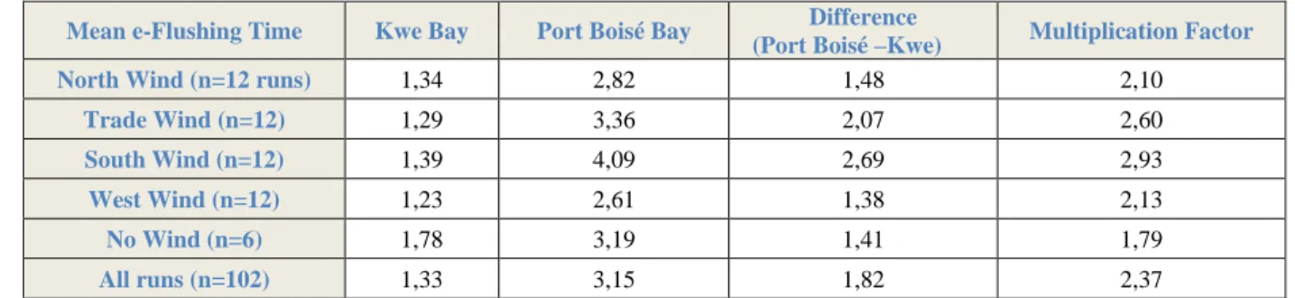
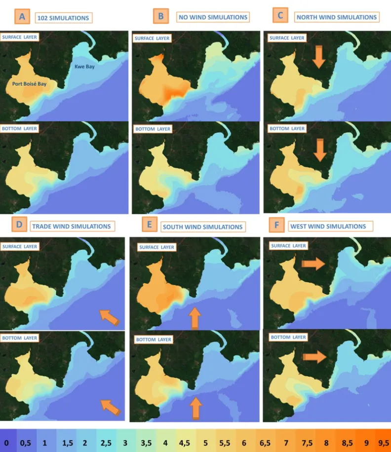
Local EFTs are presented here as a function of physical forcings applied to the various simulations. Figure 4 shows the spatial distribution and vertical variability of eFTs in Kwe and Port Boisé bays for 6 different meteorological forcings at the surface and at the bottom of the modeling grid. Each eFTs map represents an average of a simulations set of a same “wind direction” forcing, but varying conditions of tidal ranges, river inputs and wind intensities. Because surface and bottom are layers at the interface with atmosphere and sediment, they are more prone to frictional forces and shear stress than the rest of the 30 sigma layers. Their behavior in response to physical forcing is therefore amplified and values illustrated in Figure 4 need to be balanced by values integrated over the vertical axis. Table 3 represents the eFTs integrated and spatially averaged over the bays in order to compare them as entities. Figure 4A presents the local eFTs averaged for the complete set of 102 simulations. It shows the global distribution of the eFTs with all forcing conditions integrated, and therefore represents the average pattern of the study site. When comparing the mean eFTs over the vertical column, Kwe Bay appears to be drained out of tracer much faster (Table 3: 1.33 days) than Port Boisé Bay (Table 3: 3.1 days). In this case, the eFTs of Port Boisé Bay are 2.37 times higher than those of Kwe Bay. The general gradient of eFTs decreases in a shore-offshore direction, except at the surface of Port Boisé Bay, where eFTs remain relatively high (7 days) in the whole bay. An opposite gradient is even observed in the alignment of Port Boisé channel where a lens of higher tracer concentration is formed.

Figure 4B represents the local eFTs averaged over the 6 “no wind” simulations (Table 1). Its purpose is to enhance the spatial variability of eFTs under the only forcing of tide and river inputs as recommended by Safak (2015). Without any stress at the atmosphere/ocean surface interface, vertical mixing is then limited to tidal currents. Distributions, at the surface and the bottom, are similar to the previous results (102 simulations), but with substantially longer local eFTs at the surface. In the bottom layer, values are much more similar to the previous case, revealing an important vertical gradient of eFTs in both bays when no wind induced currents occur. Table 2 indicates vertically averaged eFTs of 1.78 and 3.19 days for Kwe and Port Boisé bays, respectively. The “no wind” simulations show the lowest multiplication factor between both bays: it takes less than twice the time needed in Kwe Bay for Port Boisé Bay to empty.

Table 3: Local e-flushing time in days, difference and multiplication factors, averaged over the vertical, for Kwe and Port Boisé bays.

As seen above, eFTs are shorter at the bottom than at the surface. At the bottom, eFTs decrease in the channel of Port Boisé Bay. The longest eFTs, and therefore stagnation “risk zones” in this condition are found in Kwe Bay near the river mouth at the surface, on the reef flat and in the river at the bottom. The effect of north winds on eFT values (Figure 4, C), when all wind intensity, tidal and river input conditions are combined, is of the same order of magnitude at the surface and at the bottom, indicating an homogeneous water column (intensified mixing). However,

Mean e-Flushing Time Kwe Bay Port Boisé Bay Difference

(Port Boisé –Kwe) Multiplication Factor

North Wind (n=12 runs) 1,34 2,82 1,48 2,10

Trade Wind (n=12) 1,29 3,36 2,07 2,60

South Wind (n=12) 1,39 4,09 2,69 2,93

West Wind (n=12) 1,23 2,61 1,38 2,13

No Wind (n=6) 1,78 3,19 1,41 1,79

12

the eFTs of Port Boisé Bay are 2.10 times higher than those of Kwe Bay (table 3). The highest eFTs are found at the river mouth of Trou Bleu River and in patches observed both at the surface and at the bottom on the reef flat in the west of Port Boisé Bay. It seems that the tracer is likely to be accumulated and trapped in this zone with a northerly wind. Trade winds (southeast winds) are the dominant wind condition in New Caledonia. They trigger similar eFT values (Figure 4D) and distributions over the bays than the averaged conditions (102 simulations), with Port Boisé Bay taking 2.6 times longer (Table 3) to clean up from the tracer than Kwe Bay.

The effect of the channels (external water intrusion) is disrupted by the effect of the southeast wind. The high concentration lens visible at the surface in the center of Port Boisé Bay shows the pushing effect of freshwater river inputs towards the reef, and the effect of trade winds stopping the transport of the tracer at the reef, making it a potential risk zone in case of pollution. Figure 4E displays the largest difference between local eFTs in Kwe and Port Boisé bays in south wind conditions, with a mean difference of 2.69 days (Table 3). South winds are responsible for the longest eFTs in Port Boisé Bay when averaged over the vertical (4.09 days). The spatial gradients “shore-offshore” for both bays are similar to the previous cases, with longer eFTs near the river mouth in Kwe Bay at the surface and at the bottom. The longest eFTs are found at river mouths and near the channel at the surface of Port Boisé Bay. The effect of west winds on the distribution of eFTs over the bays is illustrated in Figure 4F. The gradients of local eFTs are very consistent with the previous cases, but the order of magnitude is the smallest compared to all other wind directions (2.61 days in Port Boisé Bay and 1.23 days in Kwe Bay). The channel of Port Boisé Bay remains the zone of the bay that is cleaned of the tracer the fastest at the bottom, but the slowest at the surface. A vertical gradient was observed with shorter eFTs as the depth increases.

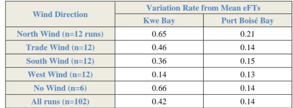
Table 4 displays the weighted standard deviation (here called “variation rate”). Table 4: Variation Rate in % (weighted Standard Deviation) integrated on the vertical for each bay.

Wind Direction Variation Rate from Mean eFTs

Kwe Bay Port Boisé Bay

North Wind (n=12 runs) 0.65 0.21

Trade Wind (n=12) 0.46 0.14

South Wind (n=12) 0.36 0.15

West Wind (n=12) 0.14 0.13

No Wind (n=6) 0.66 0.14

All runs (n=102) 0.42 0.14

Port Boisé Bay eFTs appear less prone to oscillations (13 to 21 % variation of the mean eFTs) than Kwe Bay eFTs (between 15 and 66 %). Kwe Bay responsiveness to changes in physical forcing is globally three times higher than Port Boisé Bay, except with the application of a west wind forcing in the simulations.

13

14

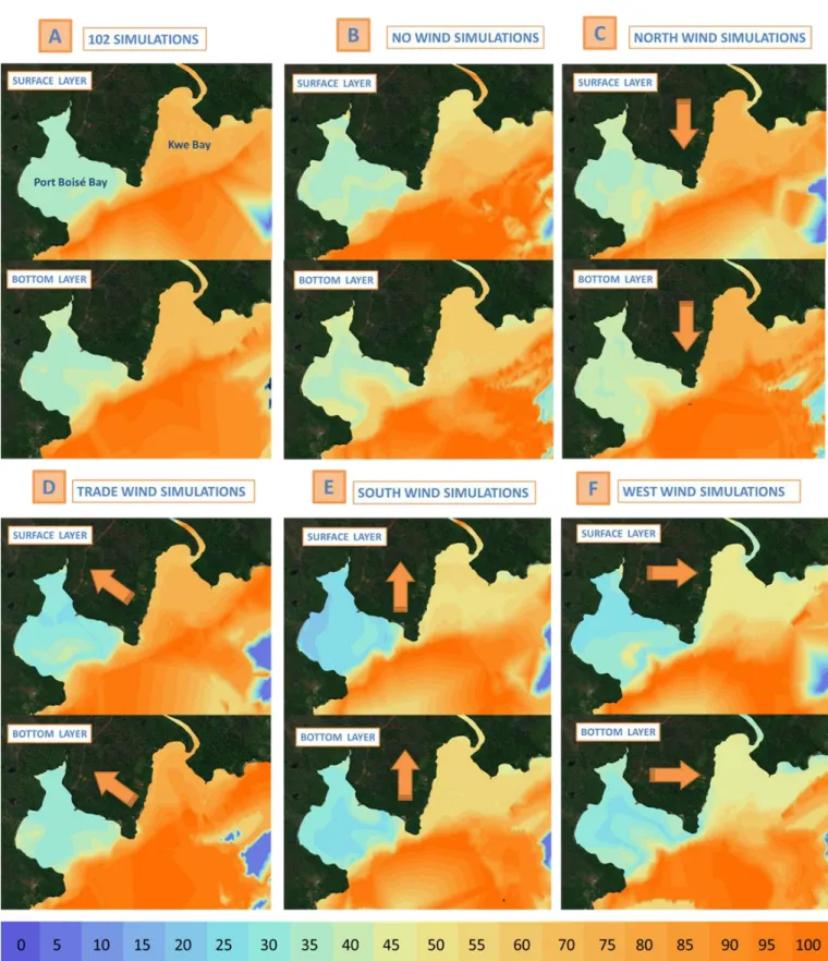
Figure 5 illustrates the spatial distribution of weighted standard deviation in eFT values. High values found offshore should not be considered as eFTs are so weak that weighted standard deviations are of the same order of magnitude, leading to 100% variation from the mean eFTs.

Maps in Figure 5 A illustrate the clear difference between the bays in term of the variation rate of eFTs, under the influence of all physical forcings. Kwe Bay is characterized by variations between 70 and 75% from averaged eFTs values, whereas they only reach 30 to 35% in Port Boisé Bay. These values peak at the interfaces (surface and bottom) because of the frictional forces applied, but the trend remains the same when the values are integrated over the vertical (Table 4). Without any wind applied, Kwe Bay still displays higher variation rates than Port Boisé Bay (Table 4: 66 % and 14 % variations, respectively).

Kwe Bay also shows a shore-to-reef gradient of variations at the surface (Figure 5B). These proportionally increase to reach their maximum near the reef, which indicates a clear influence of the tidal range variability on eFT values. Port Boisé Bay variations are much more homogeneous within the bay at the surface, and at the bottom, the effect of the channel, and its part in external water ingress, is clearly visible. Without wind forcing, variations are proportional to the turbulence induced by tidal currents and river inputs. North winds trigger variations much more important in Kwe Bay than Port Boisé Bay (Table 4: 65% and 21%, respectively).

North winds trigger the highest variation rate in Port Boisé Bay compared to other wind conditions (Figure 5C), and as such constitutes the hardest wind condition for risk assessment because of the high variability it induces in eFTs. Trade winds (Figure ED) variations are relatively high for Kwe Bay and low for Port Boisé Bay (Table 4: 46% and 14%) meaning that variability of tidal conditions, river inputs and wind intensity have a major impact on Kwe Bay but not on Port Boisé Bay hydrodynamics.

Figure 5E illustrates that over the set of south wind simulations, eFTs show a low variability in Port Boisé Bay (Table 4: 15 %) and a moderate variability in Kwe Bay (36%).

West winds are the second scenario where standard deviations are higher for Port Boisé Bay than Kwe Bay. It is also the only scenario where variation rates are similar in Port Boisé Bay (13%) and Kwe Bay (14%) (Figure 5F). West winds induce the shortest eFTs and the lowest variations due to physical forcing changes.

15

Figure 5: Variations from the mean eFTs in %, due to physical forcing variability (tidal range, river inflow and wind intensity, for each wind direction considered.

16

3.2. Zonal comparison of physical forcing effects

The maps presented in Figures 4 and 5 result from several simulations forced with the same wind direction. They identify the potential stagnation cells or zones but represent an average of different wind intensities, river inputs and tidal conditions. The radar diagrams in Figure 6 allow the distinction of the different forcings by zone (as described in Figure 2). EFTS values are overlaid on the radars for two wind intensities (5 m/s displayed in bleu and 8m/s displayed in red) with respect to the wind direction (displayed in °, in a clockwise direction). The eFTs values are integrated vertically and over the 3 tidal cycle conditions (LTR, MTR, HTR). Zones 1, 2, 3 and 4 characterize Kwe Bay, whereas zones 5, 6, 7 and 8 represent the different areas of interest in Port Boisé Bay (Figure 2).

3.2.1. The impact of wind conditions under Medium River Flow

The scales of the radars in Figure 6 have been adjusted according to the order of magnitude of eFTs found in each Bay. In Kwe Bay, with a medium flow of freshwater from the rivers, local eFTs do not exceed 2 days independently of the zone, wind direction or intensity. Although Zone 2 appears to be the fastest zone to clean up from the tracer, and zone 4 to be the slowest, the order of magnitude is similar for the four zones. An increase in wind intensity of 3 m/s produced shorter eFTs for every zone, due to intensified vertical mixing and enhanced diffusion. The variability of the wind direction also has more impact on local eFTs when the wind velocity is higher. For winds of 5 m/s, eFTs are of the same order of magnitude whatever the direction (octagonal radars); for winds of 8 m/s, differences in eFTs can be noticed. The shortest eFTs in Kwe Bay are measured with sustained northeast (60°) and southwest winds (225°). The longest eFTs are measured with southeast winds (135°), except in zone 4 with fast winds (8 m/s) and where the longest eFTs are measured with northwest (270°) winds. The fastest eFTs are observed when the wind blows side shore, whether with high or low velocity, while the longest eFTs are measured with on-shore southeast winds.

17

Port Boisé Bay shows more heterogeneous eFTs between zones. Independently of wind direction, zones 5 and 6, need more time for the tracer to disappear (min=2.25 and max=5.75 days) than zone 7 (min=1.91 and max=4.11 days) and zone 8 (min=0.57 and max=2.44 days). In zones 5 and 6, more intense winds result in longer eFTs, while zone 7 shows limited impact of wind intensity variations on eFTs. The scale of eFTs and the impact of wind intensity and direction on eFTs in zone 8 (Port Boisé Bay) is similar to those of Kwe Bay. For zones 5, 6 and 7, the highest eFTs are observed with strong south (180°) winds and the lowest with strong northwest (315°) winds. As in Kwe Bay, winds of 5 m/s in Port Boisé Bay have no major influence on eFTs as they are substantially similar for all directions. Interestingly, zone 1, which is located at the bottom of Kwe Bay harbors eFTs faster than those of zone 4, which is located at the entrance of the bay. Although the freshwater inputs at the bottom of the bay contribute to the dilution of the tracer in zone 1, the difference highlighted here is due to the successive arrival of tracer in downstream zones, which increases eFTs through the maintenance of high tracer concentration.

This observation can only be made by considering the local eFTs, which emphasizes the accumulation of tracer in a zone, independently of its origin. The effect of wind direction on the variability of local eFTs is significant only from a threshold wind intensity. Below this threshold only the tidal cycle, river flow and geography of the zone may have an influence. Unlike Kwe Bay, the zones of Port Boisé Bay are characterized by eFTs proportional to their respective distance to the reef, and therefore to the main source of water renewal. Zones 5 and 6, at the bottom of the bay, are the slowest to drain, the channel (zone 7) is much faster and the reef flat (zone 8) is where the tracer is diluted the fastest. This may be explained by the smaller flows of the creeks and Trou Bleu River into Port Boisé Bay compared to the Kwe River flow, leading to limited mixing and dilution from freshwater in zones 5 and 6. In addition, zones 7 and 8, which already benefit from the proximity of oceanic water, also avoid massive tracer arrival from zones 5 and 6. The lower general dynamics in Port Boisé Bay, which leads to longer eFTs, can also be explained by larger depths and the wide and enclosed shape of the bay.

3.2.2. Impact of wind conditions under Low River Flow

The response of local eFTs to a decrease in freshwater inputs by rivers was also studied by running the same simulation than above but with low flow river inputs. We observed that, independently of the scenario considered (wind direction and intensity), the four zones of Kwe Bay have larger eFTs than for a medium river flow, but the radar diagrams remain relatively similar in shapes. This can be linked to the lower amount of freshwater discharging in the bays, leading to a slower dilution of the tracer. However, this does not interfere with the respective effects of wind direction and velocity on eFTs. The longest local eFTs in Kwe Bay (1, 2, 3 and 4) were observed with moderate southeast (135°) winds and the shortest with strong northeast (60°) winds. In Port Boisé Bay, maximum eFTs were observed in zone 5 and 6 with 8m/s south winds and medium river flows. With low flows, the two maximum values of eFTs are obtained with a 5m/s south wind (6.47 days) and with a 8m/s southwest wind (6.48 days), while the shortest eFTs were triggered by strong north (0°) winds. The same observations were made for zone 7 in Port Boisé Bay, at a smaller scale (min=1.91 and max=4.33 days). Zone 8 has different dynamics as its longest eFT is observed with strong north winds and its shortest with strong south winds. The variability of zones 5, 6 and 7 demonstrates the concomitant effect of wind direction and intensity, that can, in one case (medium flow) induce long eFTs when winds are stronger, and in another case (low flow) induce long eFTs when winds are weaker.

In the majority of the cases considered, low river flows induced longer local eFTs. However, the opposite can happen, especially with high velocity trade and southeast winds. Zone 6 was the most impacted by a decrease in river flow under these very specific conditions (decrease of 1.04 and 0.96 days by strong trade and southeast winds, respectively). But for other wind directions, zones 5 and 6 are the most likely to an increase of their eFTs with a decrease of river inputs.

18 3.2.3. Variation rates due to wind conditions variability

Having determined the local eFTs with respect to specific wind directions, the next step was to quantify the impact of wind direction variability on eFTs values. Table 5 shows the mean variation rates of eFTs by zone, induced by changes in wind direction (n=8 directions, as described in Table 1) for two river flow conditions and two wind intensities. For all zones, variation rate doubles as the wind intensity rises from 5 to 8 m/s. For a moderate wind (5 m/s), the eFTs of the zone are therefore fairly similar whatever the direction of the wind (low variation rates: between 6 and 25 %). For a more intense wind (8 m/s), changes in wind direction will have an impact on the mixing intensity and/or accumulation of the tracer, causing the variations of eFTs to rise up to 56%. Zone 8 shows the strongest sensitivity with variations tripling as the wind intensity increases. River flows, on the other hand, have no concomitant effect with wind direction variability as variations rate are sensibly alike with medium or low flows. Table 5: Mean variation rates (in %) from the mean eFTs due to changes in wind directions (n=8)

River inputs Wind Intensity Zone 1 Zone 2 Zone 3 Zone 4 Zone 5 Zone 6 Zone 7 Zone 8

Medium Flow (n=48) 5 m/s (n=24) 0,12 0,14 0,14 0,6 0,14 0,16 0,13 0,14 8 m/s (n=24) 0,22 0,24 0,23 0,15 0,34 0,31 0,28 0,51 Low Flow (n=48) 5 m/s (n=24) 0,11 0,14 0,15 0,7 0,25 0,22 0,17 0,18 8 m/s (n=24) 0,20 0,24 0,25 0,23 0,33 0,36 0,31 0,56

Table 6 sums up, for every zone, its mean eFTs and sensibility to each physical forcing (river flow, wind intensity or wind direction). It clearly demonstrates that the channel of Kwe Bay (zone 2) has the highest water renewal rate (lowest eFTs), when all physical forcings are considered, whereas zones 5 and 6 compete for the lowest water renewal rate. They are most prone to the risk of stagnation and accumulation of a potential pollutant or contaminant. For all zones considered, west winds trigger the shortest eFTs, and south wind the longest.

Table 6: Averaged eFTs in days and variation rates associated, by zone and for all physical forcings, all tidal range conditions included

Forcing Zone 1 Zone 2 Zone 3 Zone 4 Zone 5 Zone 6 Zone 7 Zone 8 All Zones

eFT Var. eFT Var. eFT Var. eFT Var. eFT Var. eFT Var. eFT Var. eFT Var. eFT Var.

Low flow (n=48) 1,5 0,39 1,2 0,53 1,3 0,49 1,6 0,31 4,4 0,14 4,3 0,14 3,2 0,1 1,7 0,25 2,4 0,29 Medium flow (n=48) 1,3 0,45 1,0 0,55 1,2 0,51 1,5 0,28 3,5 0,14 3,7 0,13 2,8 0,11 1,7 0,24 2,1 0,30 5 m/s Wind (n=48) 1,6 0,54 1,3 0,67 1,5 0,61 1,8 0,35 3,9 0,17 4,0 0,14 3,1 0,11 2,0 0,28 2,4 0,36 8 m/s Wind (n=48) 1,2 0,19 0,8 0,26 0,9 0,27 1,3 0,19 4,0 0,13 4,0 0,13 2,9 0,09 1,3 0,17 2,0 0,18 North Wind (n=12) 1,3 0,67 1,2 0,78 1,3 0,73 1,6 0,48 3,2 0,23 3,1 0,21 2,4 0,22 2,5 0,18 2,1 0,44 Trade Wind (n=12) 1,4 0,45 1,1 0,54 1,2 0,62 1,5 0,30 4,4 0,12 4,4 0,13 3,4 0,08 1,3 0,38 2,3 0,33 South Wind (n=12) 1,7 0,34 1,2 0,46 1,3 0,40 1,4 0,26 5,6 0,17 5,6 0,13 4,0 0,11 1,2 0,19 2,7 0,26 West Wind (n=12) 1,2 0,15 0,9 0,22 1,1 0,15 1,7 0,09 3,3 0,17 3,3 0,11 2,3 0,09 1,5 0,13 1,9 0,14 No Wind (n=6) 1,8 0,65 1,6 0,84 1,7 0,73 2,0 0,47 3,8 0,06 3,8 0,06 3,1 0,14 2,2 0,41 2,5 0,42 All runs (n=102) 1,4 0,41 1,1 0,54 1,2 0,50 1,6 0,30 3,9 0,14 4,0 0,13 3,0 0,11 1,7 0,25 2,2 0,30

19

Variation rates in Table 6 show the sensitivity of each zone to changes in forcing conditions. Highest eFT variations are, inversely to eFT values, found in zone 2 (Kwe Bay channel) and, generally, Kwe Bay is more prone to large eFT variability than Port Boisé Bay. Nevertheless, the smallest variations are not found for zone 5 nor 6, but for zone 7 in Port Boisé Bay. Surprisingly, the highest variation are found in zone 2 (54% on average over all simulations) and the lowest variation in zone 7 (11 %), respectively corresponding to the channels of Kwe Bay and Port Boisé Bay. All zones combined, north winds lead to larger variations in wind intensity and river input changes. When west winds are applied, variations are the most limited.

3.3. Influence of tidal cycle and amplitude on the variability of local eFTs

The ability of the model to reproduce sea surface elevation was proven by comparing measurements and modeled SSE. The resulting correlation coefficients (R², at the five sites considered, were the following: 0.912; 0.94; 0.924; 0.915; 0.908. These high correlation values indicate that the model in our configuration provides very satisfactory calculations of SSE due to tidal cycles in space and time. The small differences are likely due to meteorological conditions (such as wind waves or river inputs) which were not accounted for in the comparative simulation.

In the radar diagrams presented above, the simulations were averaged over the 3 different runs realized with different tidal ranges: LTR, MTR and HTR. Here, we considered three identical simulations, with medium river flow and without any wind forcing, successively run to match these three different stages of the tidal cycle. Figure 7 illustrates the significant differences between eFTs values, induced by different tidal ranges during the simulations. When the simulation ran during a LTR, discrepancies among eFT zones were limited (less than one day). Kwe Bay values were very similar, close to 3 days for all four zones. The four other zones show more variability, with zones 5 and 6 still showing the longest eFTs (3.5 days), and zone 8 being similar to the zones of Kwe Bay. When the simulations ran on a MTR or HTR, most local eFTs decreased substantially for Kwe Bay and differences among the zones are significant (up to 1 day). Intense tidal currents induced larger spatial differentiation of eFT values. Kwe Bay appeared to be much more influenced by tidal currents and more prone to important variability of eFTs under physical forcings than Port Boisé Bay. Figure 7 emphasizes the significant effect tidal range (LTR, MTR, and HTR) can have on the variability of eFTs.

Figure 7: Comparison of local eFTs (in days) for No Wind simulations, run at different states of tidal range for each zone

Variation rates of eFTs values, due to changes in tidal range, were considered for both sets of simulations described in Table 2, and displayed in Figure 8. It appears that local eFTs only fluctuate up to 30 % from the mean eFTs. The

20

two sets of simulations give very similar variation rates for Port Boisé Bay, where variations do not exceed 20% of the mean eFTs except above the channel. In contrast, in Kwe Bay, variations of eFTs values range from 40 to 50 % when considering the effect on tidal range monthly variation (Figure 8A). On the other hand, the effect of the diurnal tidal cycle in Kwe Bay leads to a very low variation rate at the surface and at the bottom (less than 20%, Figure 8B). Substantial variations outside the reef are due to minimal values of averaged eFTs (a few hours) which may result up to 100% variation.

Figure 8: Variations in eFTs (in days) of the 28 simulations without wind, run every 12 hours (A), and of the 24 simulations without wind, run every hour for a day (B), for the surface and bottom layers

4. Discussion

4.1. Spatial distribution of local eFTs

The maps in Figure 4 show the spatial distribution of local eFTs and provide an overview of stagnant and dynamic regions. No matter the forcing conditions, the horizontal gradients of eFTs decreased from shore to reef. This pattern reflects the intrusion of water from outside the bays under the general effect of tides and winds, and the increased mixing they induce. Most of the water exchange (entrance/exit) is done through the channels of both bays. A smaller part of internal water is renewed with the entrance of water over the fringing reef at rising tide, and with the exit of water by the channels at ebbing tide.

Local e-flushing times were significantly higher in Port Boisé Bay, making it a potential zone of enhanced stagnation of water masses, compared to Kwe Bay. The tracer is mainly accumulated at end of bays but also trapped in a local eddy in Port Boisé Bay, formed by opposing wind-induced and tidal currents. This zone represents a “passing zone”

21

through which water draining from other areas of the bay passes before emptying offshore. Its position fluctuates slightly according to the wind direction. This stagnation zone is to be monitored in case of pollution. The maps also demonstrate a clear vertical variability in local eFTs values. In all the simulations, for both bays, eFTs are longer at the surface, meaning a more intense mixing and a quicker renewal at the bottom. The most important vertical gradient of eFTs in both bays happens when no wind forcing is applied. Without wind stress, mixing is very limited in the surface layer and amplifies the vertical gradient of local eFts. The analysis realized over the whole set of simulations identified the difference in water renewal rate between the bays; Port Boisé Bay is characterized by eFTs 2.37 times higher than Kwe Bay (Table 2), making it a potential zone of enhanced stagnation of tracer, compared to Kwe Bay. This global pattern of eFTs distribution is shown to vary depending on the tidal and meteorological forcings applied, and the order of magnitude also varies significantly; the high concentration lens visible above Port Boisé channel is amplified under the effect of trade wind stopping the exit of the tracer. Simulations run without wind forcing trigger the longest eFTs in Kwe Bay, especially at the surface. Turning off the wind forcing also increases local eFTs in Port Boisé compared to the results obtained with wind forcings, in accordance with Safak et al. (2015). The intensity of the wind is the key factor to its effectiveness at governing zonal dynamics, and, therefore, their characteristic eFTs. Indeed, the wind acts as a forcing by the square of its velocity; a 8 m/s wind will have an impact 2.5 times higher on the water surface than a 5 m/s wind.

South wind conditions triggers the largest differences in local eFTs between the bays and are responsible for the longest integrated eFTs in Port Boisé Bay (4.09 days). The order of magnitude of the local eFTs is the minimal with west winds. One possible explanation is that west winds amplify the transport of tracer towards the lagoon, leading to noticeable lower local eFTs. Inversely, south winds confine surface water to the bays, increasing eFT values. The shortest eFTs are observed when the wind blows side shore, exerting a pull force on water masses in both bays, and causing them to flow out. The longest eFTs are observed with on-shore southeast winds, pushing water masses towards the bottom of the bays and slowing down the elimination of tracer.

EFT values do not only depend on the turbulence level of the water mass in question. They result from two different phenomena: the time needed for external water to reach a given volume and dilute its tracer concentration, and the arrival of tracer from surrounding volumes being drained. Stagnation zones can, therefore, be areas of poor dynamics or/and passing areas receiving additional tracer concentration from other zones. However, this study and the eFTs analysis are based upon the hypothesis that the potential pollutant comes from mining industry, thus flows into the bays from the rivers. Stagnation zones highlighted in this study arise from this postulate. With the assumption of a similar dissolved and passive pollutant coming from offshore, stagnation zones in the bays would most likely be located otherwise.

Consideration of weighted standard deviation (variation rate) over the study site proves that eFTs values in Port Boisé Bay are less prone to oscillations (13 to 21 % variation of the mean eFTs) than Kwe Bay eFTs (between 15 and 66). Comparison of values integrated over the vertical (Table 4) and maps of surface and bottom layers (Figure 5) shows high variation rates of interface layers (surface and bottom, directly undergoing physical forcings) but moderate values over the vertical. It illustrates the need to consider the integrated values over the whole water column in order to obtain correct data about susceptibility of the bay to a specific set of forcings. It also allows high variability zones to be identified, where the risk of stagnation only appears under specific conditions. This underlines the necessity of considering residence time in relation to immediate meteorological forcing, rather than with average weather conditions.

22

4.2. Zonal comparison of physical forcing effects

As seen on the radar diagrams (Figure 6), local eFTs generally increase with low river flows and shorten with higher river inputs. The influence of wind direction is almost identical for most zones: moderate winds induce longer eFTs than strong winds. However, three zones stand out regarding the impact of wind intensity on eFTs: in zones 5, 6 and 7, winds of 8 m/s increase the eFTs. The greater depth and the sheltered locations of these zones are the possible reasons for their weak responsiveness to wind and tide conditions. Zones 1, 2, 3, 4 and 8 are the most reactive to the intensification of the wind. Their dynamics are more influenced by the wind-induced currents than by tidal currents when wind reaches a threshold velocity. For each zone, a threshold value exists, above which wind conditions overtake the other physical forcings on defining the eFT zones. A complementary work could be undertaken to determine this critical value with a systematic study for each wind direction, river flow and tidal range considered. Zonation of the bays into 8 areas clearly demonstrates the spatial variability of local eFTs values due to the geometry and the bathymetry of the bays. Zones 5 and 6, confined at the end of Port Boisé Bay, are most prone to the risk of stagnation and accumulation of a potential pollutant or contaminant. Kwe Bay and Port Boisé Bay are equivalent in size, but their respective volume and response to forcings variability indicate that Kwe Bay hydrodynamics are predominantly defined by changing meteorological forcings (wind changes, fluctuations in river inputs). Conversely, Port Boisé Bay hydrodynamics are mainly determined by cosmic forcings (tidal currents) and changing meteorological forcings are not key to its water mass movements.

In order to retrieve the sensibility due to tidal stage and range, identical scenarios were run at different instants of the tide, with no wind conditions applied. The variation rates from the sets of the 24 and 28 simulations were retrieved to get the sensibility of eFTs to diurnal cycle and to tidal range, respectively (Table 7). Variability in eFT values due to natural changes in tidal range over a lunar cycle stands between 25 and 48% in Kwe Bay compared with 4 to 25% in Port Boisé Bay. Variability due to the diurnal tidal cycle ranges between 2 and 13% for both bays. Its influence is, therefore, considerably less significant than the tidal range variations on eFT values (alternating spring and neap tides). Tidal range must be taken into account for the calculations of critical eFTs in the case of a contamination in order to refine the determination of potential risk zones.

Table 7: Integrated eFTs (days) and variation (%) for each zone and over the vertical for both sets of “No wind” simulations

Simulation set Zone 1 Zone 2 Zone 3 Zone 4 Zone 5 Zone 6 Zone 7 Zone 8

28 Simulations (every 12 hours within 14 days) eFTs 1.67 1.39 1.49 1.89 3.31 3.28 2.84 2.27 Variation rate 0.37 0.48 0.41 0.25 0.05 0.04 0.07 0.25 24 Simulations (every hour within

24 hours)

eFTs 2.03 1.76 1.85 2.20 3.32 3.32 2.96 2.63

Variation

rate 0.11 0.13 0.10 0.05 0.02 0.04 0.06 0.12

5. Conclusion

This study proposes a modeling method using residence times as indicators of stagnation zones. The hydrodynamic time parameters used were meant to enhance the longer residence time areas of a studied zone and, therefore, allow the predication of potential stagnation areas or “risk zones” in the case of contamination. These areas vary according

23

to tidal and meteorological conditions of the simulations, particularly wind direction. The shortest and longest eFTs allows the distinction between hydrodynamic and stagnant zones, respectively, as a function of the physical forcings. The use of a decreasing exponential equation to calculate the residence time from tracer concentrations was shown to be adequate. Nevertheless, highly hydrodynamic zones appear to be the most difficult for reproducing eFTs using a simple exponential equation.

Spatial variability of local eFTs was evidenced, horizontally and vertically, and partly explained by the geometry of the modeled domain and its bathymetry. However, the general pattern of eFTs values is shown to vary as a function of physical forcings, especially wind conditions. The local eFT variability was significantly impacted by wind direction above a threshold intensity. For each zone, a threshold value might be determined, above which wind conditions overtake the other physical forcings in defining the eFT zones, and below which mainly tidal cycle, river flow and the geography of the zone may be influential. When wind forcing disappears, the influence of tidal range variability is very strong on eFT values. River flow variability has an impact on eFTs, with a global increase of eFTs in every zone when river flow decreases. However, the opposite can happen, especially with high velocity trade winds and southeast winds. The influence of tides was addressed, and the variation rates in eFTs due to the diurnal tidal cycle have been shown to be much lower than those due to tidal range changes over a lunar cycle. A diurnal cycle of tides (alternating ebbing and rising tides) induces less variability in eFT values than oscillation of the tidal range over a lunar cycle (neap tide and spring tide alternation).

Long local eFTs are not necessarily linked to zones of weak dynamics but can be caused by conflicting forcing effects (opposing wind and tide currents) or by the geographical position of a zone (passing zones). Antagonistic surface phenomena, (wind at the surface, accumulation in passing zones, shoreline and bathymetry, river inputs …) can have concomitant or opposing effects on that dissolution by wind-induced or tidal currents and turbulence. This underlines the need to consider residence time with regards to meteorological forcings, rather than with average weather conditions.

Weighted standard deviations of local eFTs (expressed in % and expressed as “variation rate”) have been monitored as they allow the identification of the high variability zones, where risks of stagnation only appear under specific conditions. These zones are sensitive to changes in tidal range, wind intensity and river input fluctuations. Variations of eFTs due to changes in weather and physical conditions are thus much more important in Kwe Bay (65%) than Port Boisé Bay (21%).

In order to illustrate the method in this contribution, stagnation zones have been highlighted within the two bays studied, as well as the riskiest weather conditions. This stagnation zones are to be monitored in case of pollution as it constitutes a risk for the surrounding environment. We showed that Kwe Bay responsiveness to changes in physical forcing is globally three times higher than Port Boisé Bay.

The methodology applied and presented in this paper uses local hydrodynamic time parameters to monitor stagnation risk areas in two tropical bays, depending on meteorological and physical forcings. This method is totally applicable and scalable to other systems and concerns, such as water quality management or deposition/erosion issues, in estuaries, lagoons of varying sizes or semi-enclosed bays, where strong temporal variability of meteorological forcing is expected. The 3D model used must be adapted to the desired scale to allow calculations of the local HTs. Our contribution showed that local e-flushing times are appropriate for their ability to evidence the spatial variability of dynamics in the target volume. In case of pollution, local eFTs gradients may highlight spatial differentiation of areas at scales as small as bays, and they can be used to identify potential stagnation zones.