HAL Id: hal-00317264
https://hal.archives-ouvertes.fr/hal-00317264
Submitted on 19 Mar 2004
HAL is a multi-disciplinary open access
archive for the deposit and dissemination of
sci-entific research documents, whether they are
pub-lished or not. The documents may come from
teaching and research institutions in France or
abroad, or from public or private research centers.
L’archive ouverte pluridisciplinaire HAL, est
destinée au dépôt et à la diffusion de documents
scientifiques de niveau recherche, publiés ou non,
émanant des établissements d’enseignement et de
recherche français ou étrangers, des laboratoires
publics ou privés.
meridionalwinds I: optical and radar experimental
comparisons
E. M. Griffin, I. C. F. Müller-Wodarg, A. Aruliah, A. Aylward
To cite this version:
E. M. Griffin, I. C. F. Müller-Wodarg, A. Aruliah, A. Aylward. Comparison of high-latitude
ther-mospheric meridionalwinds I: optical and radar experimental comparisons. Annales Geophysicae,
European Geosciences Union, 2004, 22 (3), pp.849-862. �hal-00317264�
SRef-ID: 1432-0576/ag/2004-22-849 © European Geosciences Union 2004
Annales
Geophysicae
Comparison of high-latitude thermospheric meridional winds I:
optical and radar experimental comparisons
E. M. Griffin, I. C. F. M ¨uller-Wodarg, A. Aruliah, and A. Aylward
Atmospheric Physics Laboratory, University College London, 67-73 Riding House Street, London W1W 7EJ, UK Received: 03 September 2002 – Revised: 25 July 2003 – Accepted: 30 July 2003 – Published: 19 March 2004
Abstract. Thermospheric neutral winds at Kiruna, Sweden
(67.4◦N, 20.4◦E) are compared using both direct optical Fabry-Perot Interferometer (FPI) measurements and those derived from European incoherent scatter radar (EISCAT) measurements. This combination of experimental data sets, both covering well over a solar cycle of data, allows for a unique comparison of the thermospheric meridional com-ponent of the neutral wind as observed by different experi-mental techniques. Uniquely in this study the EISCAT mea-surements are used to provide winds for comparison using two separate techniques: the most popular method based on the work of Salah and Holt (1974) and the Meridional Wind Model (MWM) (Miller et al., 1997) application of servo the-ory. The balance of forces at this location that produces the observed diurnal pattern are investigated using output from the Coupled Thermosphere and Ionosphere (CTIM) numeri-cal model. Along with detailed comparisons from short pe-riods the climatological behaviour of the winds have been investigated for seasonal and solar cycle dependence using the experimental techniques. While there are features which are consistent between the 3 techniques, such as the evidence of the equinoctial asymmetry, there are also significant dif-ferences between the techniques both in terms of trends and absolute values. It is clear from this and previous studies that the high-latitude representation of the thermospheric neutral winds from the empirical Horizontal Wind Model (HWM), though improved from earlier versions, lacks accuracy in many conditions. The relative merits of each technique are discussed and while none of the techniques provides the per-fect data set to address model performance at high-latitude, one or more needs to be included in future HWM reformula-tions.
Key words. Meteorology and atmospheric dynamics
(ther-mospheric dynamics), Ionosphere (ionosphere-atmosphere interactions, auroral ionosphere)
Correspondence to: E. M. Griffin
1 Introduction
1.1 Previous climatologies
Most climatological work on thermospheric winds has been undertaken using long-term databases from individual Fabry-Perot Interferometer measurements of Doppler shifts of auro-ral and airglow emissions, primarily the 630 nm atomic oxy-gen red line emission which has a peak emission altitude of around 240 km. The nature of the operation of the FPI instru-ment means there are limits to the diurnal and seasonal cov-erage. The FPI can observe the weak airglow emission above the background only during dark, night-time conditions. In addition, the sky must be cloud-free, otherwise light scat-tering will lose the directional information. Figure 1, from a previous climatology of neutral winds at Kiruna by Aru-liah et al. (1996a), shows the average meridional winds from the FPI at Kiruna split into separate solar cycles. The main observations in wind patterns at this latitude are northward winds by day and southward winds at night. These are the characteristics of a single site rotating with the Earth under an anti-sunward flow driven by pressure gradients caused by solar heating and high-latitude auroral heating. The night-time southward velocities are higher than the daynight-time veloc-ities due to the lower ion drag (considered here as the ions re-tarding the neutrals) encountered after sunset in the absence of photo-ionization, with consequently lower ion densities. The conclusion from this data set is that there are signifi-cant differences between the solar cycles concomitant with the differences in solar activity for each cycle.
Examples of other FPI-based climatologies include Biondi et al. (1999), who presented climatologies for low latitudes using a database running from 1980 to 1990 and Killeen et al. (1995), who presented polar cap climatologies using a shorter period from 1985 to 1991. Biondi et al. (1999) compare their data to Thermosphere Ionosphere Electrody-namics General Circulation Model (TIEGCM) output, while Killeen et al. (1995) compare to both HWM (Hedin et al., 1991) and Vector Spherical Harmonic (VSH) (Killeen et al.,
Fig. 1. A comparison of average meridional winds at solar
mini-mum from FPI measurements (north look direction) at Kiruna for 2 different solar cycles (21 and 22).
1987) predictions for their latitudes. However, neither of these studies has had the benefit of direct comparison with measurements from other types of instruments using differ-ent methodologies.
While FPIs provide the most reliable source of direct mea-surements, the low number of these instruments and the lim-itation to clear, dark skies means many other techniques have been employed to estimate neutral winds using alter-native instruments. The coupled nature of the ionosphere-thermosphere system allows for the influence of the neutral wind to be inferred from ionospheric measurements. For incoherent scatter radars (ISRs) the winds are usually in-ferred from ion velocity measurements parallel to the mag-netic field. The difference between the calculated diffusion velocity and the measured velocity component is attributed to the neutral wind. In the case of ionosonde measurements the influence of the neutral wind is gauged by application of servo theory which describes the altitude changes in hmF2, expected as neutral winds force ionization into field parallel motions. The application of these techniques to ISRs and ionosondes has allowed for the database of neutral winds to be greatly extended (e.g. Miller et al., 1997; Duboin and Lafeuille, 1992; Buonsanto, 1990, 1991). As an example, the Millstone Hill ISR database has been used to produce com-parisons for particular intervals (Buonsanto et al., 1997a) and to test the influence of changing parameters on the derivation of winds from ionospheric data (Buonsanto et al., 1997b). Recently it has been used to produce a climatology of neu-tral winds at mid-latitudes (Buonsanto and Witasse, 1999).
Most studies of optical and radar derived winds from co-located instruments are confined to periods of a few days. Dyson et al. (1997) use FPI and Digisonde derived winds observed from March 1995 at Beveridge, near Melbourne, Australia, and compare two methods for neutral wind deriva-tion from ionosonde hmF2 data with HWM93 model output.
The HWM93 output for the thermosphere is identical to that produced by HWM90. The HWM93 model winds agree rea-sonably well in overall magnitude with the winds from hmF2 for 2 March, but are about a factor of 2 smaller than the
hmF2 winds near local midnight on 3 and 4 March, which
had more geomagnetically disturbed conditions. FPI winds on these nights were in close agreement with the hmF2 de-rived winds. Relatively little Southern Hemisphere data have been included in the HWM93 model which largely accounts for the limited success.
Neither the Buonsanto et al. (1997a) nor the Dyson et al. (1997) studies use any electric field correction to the winds derived from hmF2 measurements. The authors justify this assumption by stating that these are mid-latitude sites with low geomagnetic activity during the experiments. Ac-cording to Buonsanto et al. (1997a), the major difference be-tween the winds was due to the heights at which the winds were obtained, with one height fixed, for the ion velocity de-terminations, and the other varying, according to the hmF2 measurements.
2 Experimental techniques
2.1 EISCAT winds using ISR method
The most common method of deriving neutral winds from incoherent scatter radar data is to compare the observed ion velocity parallel to the Earth’s magnetic field, together with calculations of the diffusion velocity along the field line, as pioneered by Salah and Holt (1974). This technique has been used with data from incoherent scatter radars at many sites (e.g. Millstone Hill, EISCAT, Saint- Santin, Arecibo), to pro-duce neutral winds. An example of the application of this technique is the EISCAT Ion Neutral Dynamics Investiga-tion (INDI) experiment which has been described in Farmer et al. (1990) and Davis et al. (1995).
A number of climatological studies have also used sim-ilar techniques to look at average meridional neutral winds from EISCAT data under various conditions (e.g. Titheridge, 1991; Witasse et al., 1998). As the Witasse et al. (1998) paper produces a climatology of neutral winds based on the standard Salah and Holt (1974) ISR technique from the EIS-CAT data, the INDI technique was not used to produce a sim-ilar climatology to avoid duplicating this work. The compar-ison of the results from these studies with those presented here will be shown in Sects. 3 and 4.
Witasse et al. (1998) follow the method described in Lilen-sten and Lathuillere (1995) to deduce the meridional com-ponent of the neutral wind. They do not multiply the O– O+collision frequency by the Burnside factor (Salah, 1993), as they take into account the conclusions of Lathuillere et al. (1997), who support a lower Burnside factor that is close to unity. Meridional winds for 13 different heights from 130 to 400 km are presented. In order to comply with the as-sumptions involved in their wind derivation, they exclude data from periods with electric fields greater than 20 mV/m,
or if the electric field measurement is unavailable they ex-clude data where the ion temperatures indicated Joule heat-ing was takheat-ing place. We compare with the meridional winds at 257 km, which are closest to the nominal peak height of the 630 nm atomic oxygen emission measured by the FPI at around 240 km (Sica et al., 1986). This is an assump-tion of the average height as the emission altitude at high-latitudes can vary from 200 km to 350 km, however, there is little change of horizontal wind with height (Smith et al., 1998). Witasse et al. (1998) also use their data from this height to compare to optical measurements (including FPI) and also in their comparison to HWM model output.
Witasse et al. (1998) no longer consider Apas a pertinent criterion for selection. This is because no significant differ-ence was found between mean winds at 257 km height for both high and low solar flux when separated into two geo-magnetic activity levels (Ap<11 and Ap>11). It is worth noting that their rejection criteria may in fact be the cause of the lack of any geomagnetic activity dependence in the data and will be discussed later.
Witasse et al. (1998) note that the classification scheme often differs between studies, for example, Duboin and Lafeuille (1992) consider two solar activity levels, above or below F10.7=100, and Hagan (1993) chooses F10.7>180 for solar maximum periods and F10.7<90 for solar minimum. The seasonal subsets in the Hagan study contain only two months each. We have chosen to use the Witasse et al. (1998) criteria, introduced by Aruliah et al. (1996a), to ease com-parison in this study, thus choosing F10.7=120 as the cutoff between high and low solar activity. The seasons are sepa-rated using the solstices and equinoxes +/−45 days, e.g. win-ter season covers the December solstice +/−45 days. 2.2 Digisonde winds using MWM
As a consequence of the mean lifetime of ionization in the F-region often being several hours, the distribution of ion-ization at any time is greatly dependent on transport by elec-tric fields and neutral winds. Embedded in the neutral atmo-sphere is an electron density profile whose peak is usually found at thermospheric altitudes, between 300–400 km. The atomic oxygen emissions observed by FPIs to measure neu-tral wind velocities have a peak emission height at around 240 km. These neutral winds affect the peak of the electron density because the electrons are confined to move along the Earth’s magnetic field lines. A poleward neutral wind will drive the peak down a field line, while an equatorward wind will drive it up. The peak may also be affected by zonal electric fields, but there is a commonly invoked assumption that at mid-latitudes, the electric fields are small and have a negligible effect. This leads to the possibility of using the difference between a measured peak and a “balance height” undisturbed peak (the peak in the absence of any neutral wind or electric field) to calculate a neutral wind velocity. The balance height is usually obtained from model output. This study uses the Meridional Wind Model (MWM) pro-duced by Miller et al. (1997), which takes the balance heights
from the Field Line Interhemispheric Plasma (FLIP) model by Richards (1991). This technique leads to the possibility of deriving the neutral winds in the thermosphere from iono-spheric measurements of hmF2 made by incoherent scatter radar or ionosonde. The high-latitude site used in this study, however, means that the mid-latitude assumption of negligi-ble electric fields is unsafe and leads to the need for these fields to be assessed when using MWM. This will be dis-cussed in detail in Sect. 2.3, in which MWM is used with EISCAT derived hmF2 data.
A feature of the MWM is its ability to process data in In-ternational Ionosphere Working Group (IIWG) format to es-timate hmF2 values and then use these values to derive neu-tral winds. Many ionosondes around the world forward their data in IIWG format to the World Data Center-C1 at Ruther-ford Appleton Laboratory (WDC-C1 at RAL). This database extends back to 1932 for the Slough/RAL ionosonde and has well over 150 instruments currently contributing. In this study data from the Kiruna Digisonde retrieved from the WDC database have been used to produce winds for com-parison with the other techniques. In order to use the MWM with this data, the daily mean Ap, sunspot number and F10.7 value for the day need to be established.
IIWG format data provides hourly data for the scaled pa-rameters, but in the process of conversion to neutral winds, some of the data will lie outside the acceptable range for the MWM and no output will be produced. For the Kiruna data, in particular, there have been a large number of nights where there have not been enough data for useful compari-son to the FPI and other neutral wind sources. In addition to this, the Digisonde was out of operation from October 1986 to January 1990 which considerably restricts the cov-erage available for comparison with the other sources sented here. For these reasons no climatological data is pre-sented here based on the Kiruna Digisonde results, however, the data is used in examples from specific periods. In par-ticular, Fig. 2 shows average derived winds from the Kiruna Digisonde monthly median data from June 1990 to Decem-ber 1991, a period of high solar activity, compared to the Kiruna FPI data from the same period, and we can see that there is very good agreement. In this case the FPI data is from periods with Kpless than 2, in order to reflect the self-filtering of the Digisonde based MWM results as described above. It does, however, point to the possibility of using the MWM, and more generally the servo theory, at this latitude, if the data is treated correctly.
2.3 EISCAT winds using MWM
The data from EISCAT experiments may also be analysed to derive values of hmF2. In this study data have been used from Common Programme experiments, predominately CP-1, stored in NCAR (after National Center for Atmo-spheric Research) format on the EISCAT project computers at RAL. Programs were written to take data in this format and produce hmF2 values by fitting a polynomial to the al-titude profile of electron density values. The polynomial is
Fig. 2. A comparison of average meridional winds at solar
max-imum from FPI measurements (blue line) at Kiruna compared to winds derived from Kiruna Digisonde measurements (red line).
then used to calculate the altitude of maximum electron den-sity, which is used as the derived hmF2 value. Values arrived at in this manner are input to the MWM, along with the rel-evant values of the various indices for the date in question, to produce output in the form of a time series of meridional neutral wind values.
These values, however, are uncorrected for the influence of electric fields. NCAR format files containing ion veloc-ity measurements with respect to the geomagnetic field are available from many EISCAT experiments, and these were used to establish the correction necessary to be applied to the winds’ output from the MWM. This is achieved by using the programs developed for the INDI experiment to derive tristatic ion velocity measurements from the EISCAT exper-iments. These are then converted to equivalent electric field values.
Previously, Buonsanto et al. (1989), using ISR data from Millstone Hill from 17–24 September 1984, derived merid-ional neutral winds from servo theory and also assessed the electric field correction to be applied to these winds using the same data. This study used the earlier work of Rishbeth (1967) and Rishbeth et al. (1978) to show that this correc-tion may be taken from the following representacorrec-tion of the poleward neutral wind (UN):
UN =(νperpNcos I − W )/(cos I sin I ), (1) where νperpNis the ion drift velocity component perpendicu-lar to the Earth’s magnetic field in the magnetic north direc-tion, I is the magnetic dip angle and W is the vertical drift in
hmF2 applied by a neutral wind or electric field under
condi-tions of diffusive equilibrium. From this equation an electric field correction, given by νperpN/sin I , can be applied to the
UNderived from servo theory. Another program was written
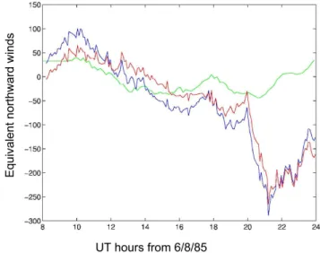
Fig. 3. This figure demonstrates the uncorrected (red line) and
cor-rected winds (blue line) from one day of an EISCAT experiment on 6 August 1985, together with the electric field correction (green line) which has been applied (all in m/s).
to take the ion drift velocity data from the CP-1 experiments and calculate this correction for the winds derived here from the hmF2 measurements.
Figure 3 shows winds from one day of an experiment on 6 August 1985, in which the red line represents the original winds derived from the EISCAT hmF2 measurements. The green line shows the correction calculated from the electric field measurements and the blue line shows the final, cor-rected winds. A running average was applied to the electric field correction values, as there is usually a lot of variability associated with the electric field measurements, and hence, they appear smoother than the derived winds in this exam-ple plot. The large inertia of the neutral atmosphere leads to confidence that this process, which is averaging over some tens of minutes, represents a realistic correction to the de-rived winds and also avoids introducing a source of greater variability to the final, corrected winds. The EISCAT-MWM winds presented later in this paper have been corrected using this method. Electric field corrections are usually small dur-ing the day but at night can be large, indicatdur-ing greater geo-magnetic activity. Geogeo-magnetically disturbed periods have been excluded by using the same filtering applied in the Witasse et al. (1998) study, i.e. electric field values must be less than 20 mV/m.
A number of studies have been published using both ionosonde and ISR measured hmF2 to derive meridional neu-tral winds. These studies have derived winds either with no electric field correction (Buonsanto, 1990) or using modelled values of electric field (Buonsanto, 1991). Subsequently, Millstone Hill ISR data have been analysed to derive neu-tral meridional winds from 34 experiments spanning August 1988 to August 1995, where corrections for the effect of elec-tric fields have been applied using ion velocity measurements
from the same experiments (Buonsanto et al., 1997b). In their study however, the data were not restricted to geomag-netically quiet times and the data were not presented in a cli-matological sense, but compared with wind results derived from ion velocities.
While previous climatologies have used techniques simi-lar to Salah and Holt (1974), (e.g. Hagan, 1993 and Witasse et al., 1998), in this paper we present the first climatology of meridional thermospheric neutral winds based on ISR mea-surements of hmF2, where contemporaneous ion velocity measurements have been used to correct the derived winds for the effects of electric fields. The data used in this cli-matology are the derived neutral winds from measured hmF2 values determined using the EISCAT CP-1 experiments with the electric field correction applied in each case. As the data from disturbed periods with large electric fields have been excluded, to match the rejection criteria invoked by Witasse et al. (1998), this then provides an equivalent climatology based largely on the same EISCAT radar database but using a different technique.
The Witasse et al. (1998) database used post-integrated CP-1 experiments which have a fixed 3-min time resolution, thus allowing them to take a simple average of the winds from each of the nights. However, we used the NCAR for-mat result files from CP-1 experiments and these contain measurements that have fixed time resolution for a specific experiment, but not from experiment to experiment. This reflects the increase in temporal resolution as the EISCAT radar was developed and improved over the years, meaning that the later experiments have higher time resolution. So, in order to ensure an equally weighted contribution to the aver-age climatology from each night, we fit a polynomial to the available data, which is then sampled for each of the hourly bins.
2.4 FPI winds - direct measurements
The database of neutral winds from the Kiruna FPI instru-ment (Aruliah et al., 1996a) has been used to produce cli-matologies and also to compare with CTIM (Aruliah et al., 1997). The location of the FPI also allows for a compari-son with several other instruments in the vicinity, including, for example, the INDI experiment, which studied ion-neutral coupling by comparing FPI and EISCAT measurements. The database has further been used to investigate the evidence of an equinoctial asymmetry in the neutral winds (Aruliah et al., 1996b).
The FPI wind climatologies for this paper use all of the data available in the Aruliah et al. (1996a) study but also include a second solar cycle. The database coverage is from November 1981 to March 1998. The data have been binned according to the scheme in Witasse et al. (1998) with F10.7=120 as the cutoff between high and low solar activ-ity and seasons separated using the solstices and equinoxes +/−45 days. This provides nighttime data for comparison with three of the four seasons in both solar activity levels commensurate with the FPI data coverage limitations
previ-ously pointed out. In particular, there are no summer FPI data because there is an insignificant length of dark conditions at nighttime for optical observations at this latitude in summer.
3 Example data
3.1 Short-term comparisons
The long-term databases of measurements come from the Kiruna FPI and the EISCAT incoherent scatter radar, which both began operation in the early 1980s, covering nearly 2 solar cycles of observations. The size and time-span of the databases from the instruments in the Kiruna-Tromsø) region allows for a wider range of intercomparisons for meridional thermospheric wind techniques to be carried out than is pos-sible for any other high-latitude site.
We have seen in the Introduction that studies by Buon-santo et al. (1997a), Dyson et al. (1997) and others have used a variety of wind derivation techniques to compare with each other and with model results over short periods. In this sec-tion we present measurements from a series of consecutive days as examples of the data that have contributed to the cli-matologies based on the various different techniques avail-able at this location. These include FPI and EISCAT hmF2 derived measurements, as well as Kiruna Digisonde hmF2 measurements, for which only data from individual nights have been derived for comparison.
Also presented are examples of neutral winds derived us-ing EISCAT data with the INDI technique. These are not identical to the winds used for the climatology developed by Witasse et al. (1998), since the techniques are independently formulated and implemented. However, the INDI winds de-rived this way will be very similar to the Witasse et al. (1998) winds since the principles are the same, and both methods use the EISCAT database.
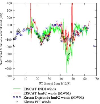
Figure 4 shows the meridional winds from 3 consecu-tive days beginning at 00:00 UT on the 8 December 1991, observed at Kiruna, which contribute to the winter season, high solar activity climatologies. Figure 4 shows the results from the 4 different methods of wind extraction introduced in Sect. 2, and the main characteristics in wind patterns at high-latitudes are demonstrated with northward winds by day and reverse flows at night. Figure 5 shows results from a series of days in late March and early April 1992 which contribute to the spring season, high solar activity climatologies. Typical characteristics of the individual techniques are demonstrated by these example plots. The best quality derived neutral wind data from the Kiruna Digisonde are during the day, as the electron densities used to produce the scaled parameters in-put to the MWM are usually higher, and consequently, more accurately observed, than at night. The EISCAT electron density data is usually available through the entire course of an experiment. However, as with the Digisonde, the accuracy of the results may be expected to drop during the night due to lower electron densities and, therefore, a poor signal-to-noise ratio which produces less consistent estimates of hmF2.
Fig. 4. Thermospheric meridional winds from four techniques for 3
consecutive days beginning at 00:00 UT on 08 August 1991.
With the FPI results the major influences on data quality are local cloud cover and the intensity of the 630 nm emission. The FPI has a fixed time resolution and hence, may sample different emission intensities for each direction, which will lead to less accurate wind determinations in directions with lower intensities. The zero Doppler shift baseline estimate for the instrument, based on averaging all directions over an entire night, means that poor data quality in one direction need not invalidate data from the other directions. Not all of the data shown in Figs. 4 and 5 will have contributed to the final climatologies as we apply filters for geomagnetically ac-tive times when the wind derivation techniques are not valid, as discussed in Sects. 2.1 and 2.2.
There are many consistent features of the data in Figs. 4 and 5. The intercomparison of winds derived from different sources of hmF2 shows very good daytime correlation, which is encouraging. As pointed out earlier this is probably due to the higher daytime electron densities allowing for a more accurate determination of hmF2 from the EISCAT ments and the scaled parameters for the Digisonde measure-ments. Buonsanto et al. (1997b) have pointed out that dif-ferences between the winds derived on individual days from the same ISR experiments using the ion velocity and hmF2 measurements could be associated with the assumption of uniform or zero gradients in the ion velocity field. In both Figs. 4 and 5 the winds derived using the MWM with input from measured hmF2 values appear to lag behind those de-rived using the INDI technique when reversals in wind direc-tion occur. This is a feature of the techniques that has been noted in a previous study (Buonsanto et al., 1989). There are also large differences in the maximum midnight southward
Fig. 5. Thermospheric meridional winds from four techniques for 4
consecutive days beginning at 00:00 UT on 30 March 1992.
winds, as seen in Fig. 5 with the winds derived from hmF2 measurements producing the greatest magnitudes and largest differences to other techniques on days when the average Ap was large.
The apparent high degree of scatter seen in the INDI de-rived winds is due to the higher time resolution of the data used by comparison with that used for the hmF2 derived val-ues, rather than an indication of lower accuracy. The NCAR format data used to derive the EISCAT hmF2 values can have different time resolution depending on each experiment. 3.2 Comparisons demonstrating response to geomagnetic
activity
Earlier, it was reported that Dyson et al. (1997) found the HWM93 model to reflect changes in geomagnetic activity quite poorly for their Southern Hemisphere mid-latitude site. However, the poor response to geomagnetic activity is also apparent in the Northern Hemisphere from both our Kiruna data and previous work at EISCAT (Kosch et al., 2000).
In Fig. 6 the HWM93 model winds are compared with directly measured winds from the Kiruna FPI and derived winds from the Kiruna Digisonde over the period 7–10 De-cember 1991. The 3-hourly Ap index indicates the sizeable variability of the geomagnetic activity. The figure illustrates that HWM93 is insensitive to changes in geomagnetic ac-tivity for a Northern Hemisphere site and thereby confirms the observation by Dyson et al. (1997). The nighttime pe-riod 18:00–06:00 UT of the 7–8 December is geomagneti-cally moderate to quiet, with a mean Ap of 8. The HWM winds fail to match the FPI maximum southward winds. The following night is very quiet with mean Ap of 4 and
Fig. 6. HWM93 model winds are compared with directly measured
winds from the Kiruna FPI and those derived winds from the Kiruna Digisonde over the period 07–10 December 1991. The top plot shows the time series of the Apindex for these days.
the HWM winds match the FPI winds to a much closer de-gree during this night. On the last night of 9–10 Decem-ber, we see that there are more disturbed conditions with a mean Ap of 14 and again the HWM winds fail to match the FPI southward midnight maximum. The daytime north-ward winds derived from the Digisonde are generally better matched by the HWM winds, which is in keeping with the Dyson et al. (1997) study, although some periods of signifi-cant difference are also evident. There is none of the system-atic overestimation of the diurnal amplitude by the HWM87 winds, as reported by Titheridge (1991), in either the Dyson et al. (1997) study or the data presented here in Fig. 6. 3.3 Format of the climatologies from the experimental
techniques
In order to investigate the longer term behaviour of the winds at our site in a climatological sense, the experimental tech-niques will be compared when separated by season and so-lar activity level. Together with winds from the Kiruna FPI, two techniques are applied to derive winds from the
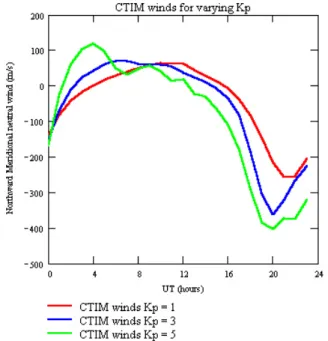
EIS-Fig. 7. A comparison showing the CTIM diurnal wind pattern for
different steady state Kplevels is shown. The red line corresponds to the Kp=1 conditions, the green line to Kp=3 conditions and the blue line to Kp=5 conditions.
CAT database, one from a previous work using the standard technique for incoherent scatter radars (Witasse et al., 1998, termed EISCAT-ISR), and a new data set derived using the MWM implementation of servo theory with the EISCAT data as input (termed EISCAT-MWM). The latter technique also uses contemporaneous EISCAT electric field data for correc-tion to the equivalent servo winds as described in Sect. 2.3.
4 Climatological Results
4.1 Theoretical variation of forces influencing neutral winds
One aspect of the difficulty in comparing results from several locations is the difference in the balance between the various forces acting to produce the overall diurnal wind pattern. For example, Buonsanto (1991) and Hagan (1993) have reported decreasing amplitudes of the diurnal meridional wind with increasing solar activity at Millstone Hill. This shows that, while pressure gradients will increase with increasing so-lar activity and kinematic viscosity decreases, the increased mass of an air parcel and increased ion drag tend to moder-ate the effect of pressure force increases and may even reduce the wind. Since there may be a rough balance between the factors tending to increase or decrease wind speed with in-creasing solar activity, these variations can be a sensitive test of theoretical models. Using first principle numerical models the measurements made at a single site can be given proper context.
Fig. 8. The ion drag acceleration through the day for the same Kp levels as in Fig. 7.
CTIM is a theoretical, self-consistent model that is de-rived from first principles. Looking at the output from this model, a comparison showing the CTIM diurnal wind pat-tern for different Kp levels is shown in Fig. 7. The model output is for high solar activity conditions (F10.7=200) in summer. The diurnal wind patterns from this model output for Kiruna are shown for three different levels of Kp, with the highest Kplevel (Kp=5) giving the greatest evidence of an early daytime poleward peak. There is also a trend toward larger southward winds at night reaching their peak earlier, at higher Kp.
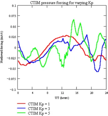
The level of geomagnetic activity is set in CTIM by ap-plying a constant average electric field model such as the Millstone Hill model (Foster, 1983). Figure 8 plots the ion drag acceleration through the day for the same Kp levels plotted in Fig. 7, while Fig. 9 plots the corresponding pres-sure gradient acceleration. Figure 8 shows clearly that ion drag becomes systematically less northward with increasing
Kpduring the period 20:00–24:00 UT and 00:00–02:00 UT. This is consistent with the meridional winds in Fig. 7 for the period 20:00–24:00 UT, but does not account for the more northward winds at high Kp in the period 00:00–04:00 UT. The answer lies in the pressure forcing which is much more variable over 24 hours at the higher Kp levels. Figure 9 demonstrates the complex balance at Kiruna between pure solar heating forcing, as is seen in the Kp=1 case, and the in-creasing influence of high-latitude auroral heating at higher
Kp values. In CTIM the combination of ion drag and pres-sure gradient forces, together with smaller contributions from the other forcing terms, such as the Coriolis effect,
advec-Fig. 9. The pressure gradient acceleration through the day for the
same Kplevels as in Fig. 7.
tion and viscous drag, produces the resultant winds shown in Fig. 7 and demonstrates the sensitivity of the model output to the chosen Kp level. A further complication arises from the modelling of geomagnetic activity. As mentioned above, the level of geomagnetic activity is set in CTIM by applying a constant average electric field model. However, the real elec-tric field has rapid, random fluctuations that are smoothed out in the electric field models. This leads to the possibil-ity that the momentum transfer from the plasma flow to the neutral winds may be overestimated, even in relatively quiet scenarios, and the underestimation of Joule heating leads to unrealistic pressure gradients.
The measured diurnal pattern from several experimental techniques is presented in the next section. Further analysis and interpretation are provided by comparing these experi-mental data to several other empirical model climatologies, i.e. the HWM and MWM models, and these are presented in the accompanying paper (Griffin et al., 2004).
4.2 Combined climatologies
In climatological studies there are subjective choices to be made in terms of the number and nature of different effects to be tested for. For this study solar cycle and seasonal crite-ria were chosen to allow for a direct comparison with Witasse et al. (1998). While other criteria, such as geomagnetic activ-ity or IMF conditions, could be envisaged to produce further categorisation, they would reduce the statistical significance of the comparisons.
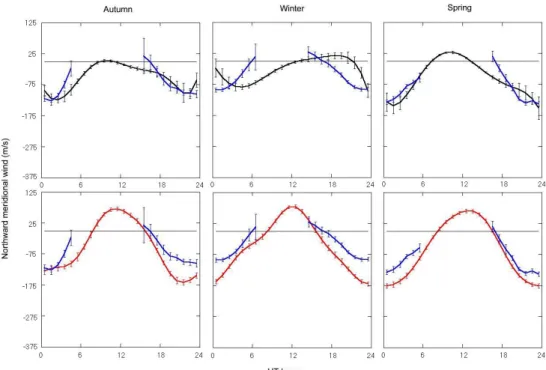
Fig. 10. Climatological comparisons for the low solar activity case with the top three plots comparing EISCAT-MWM (black lines) to FPI
climatologies (blue lines) and the bottom three plots comparing EISCAT-ISR (red lines) to FPI climatologies for each of three seasons.
Hagan (1993) showed that for the winter season at solar minimum there was a significant difference in the average diurnal wind profiles at different geomagnetic activity levels, within a data set already restricted to geomagnetically undis-turbed conditions. Witasse et al. (1998), however, found that their winds displayed no significant difference when split into separate categories of Ap>11 and Ap<11 for high so-lar activity. They also tested at low soso-lar activity and came to the same conclusion. In their case, however, their ex-periments already excluded geomagnetically active data, in order to comply with the requirement for diffusive equilib-rium when deriving neutral winds from ion velocities. This is an important factor because local, contemporaneous data have been used to mask out disturbed conditions, rather than global indices averaged over several hours. While in gen-eral thermospheric neutral winds will react to changes in ge-omagnetic activity, e.g. over periods of days, as shown in Figure 5, using the current Ap or Kp indices to separate periods of differing geomagnetic activity for climatological purposes appears to be an insensitive method of categorisa-tion. The winds for times with identical current Ap or Kp may be substantially different dependending on the preced-ing conditions (Aruliah et al., 1999). The fact that Witasse et al. (1998) still find a significant number of days included in their data with Ap>11 implies that moderate to active days, as indicated by the Apindex, may in fact display quiet time behaviour. This is due to the memory of previous levels of activity that is retained owing to the inertia of the thermo-sphere. A full method of categorisation needs to take into account any influence of geomagnetic history for individual days. Without such a selection procedure, the average effect
of geomagnetic history is likely to skew the average winds to-wards previously quiet conditions since Kp<3 for over 70% of the time (Foster et al., 1986).
In recent years there has been much debate over the na-ture of the seasonal response of the meridional thermospheric neutral wind with respect to the equinoxes and whether the diurnal patterns are the same for both spring and autumn (Aruliah et al., 1996b; Biondi et al., 1999). Both Aruliah et al. (1996b) and Witasse et al. (1998) have found that there exists an equinoctial asymmetry for the winds from the Tromsø/Kiruna location. No significant equinoctial asymme-try is predicted by either thermospheric or ionospheric model simulations, which assume that the equinoxes are fundamen-tally the same; their seasonally varying forcing functions be-ing symmetric about the equinoxes.
The results from the three measurement-based tech-niques, are compared in this section, i.e. EISCAT-ISR, EISCAT-MWM and FPI, with the EISCAT based techniques including data from January 1984 to March 1995, the FPI data from between November 1982 and March 1998. Fig-ure 10 shows the comparisons for the low solar activity case with the top three plots comparing EISCAT-MWM to FPI cli-matologies and the bottom three plots comparing EISCAT-ISR to FPI climatologies. The point for each hourly bin is plotted at the half hour position. Figure 11 presents compar-isons in the same manner but in this case for high solar activ-ity. There are no plots from the summer season as there are no FPI data available to use in such a comparison. The data compilation process allows for the calculation and display of the standard error on the mean from each of the techniques.
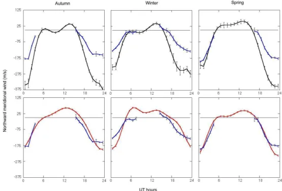
Fig. 11. As for Fig. 10 but in this case for high solar activity.
4.3 Low solar activity climatologies (F10.7<120)
At low solar activity it is reasonable to expect that the mean wind will be less northward as a result of smaller pressure gradients from lower solar flux levels. However, lower solar activity also means a statistical decrease in particle precipita-tion and photoionizaprecipita-tion. The resultant variaprecipita-tion in ion drag could produce a correlation between the maximum nighttime southward wind and solar activity. At solar minimum Hagan (1993) suggests that auroral heating to the north of Millstone Hill drives southward circulation which is strong enough to compensate for the northward circulation that is driven by in-situ solar heating. There are many discrepancies between these previous studies, however. Igi et al. (1999) report that the diurnal amplitude at Kokubunji, Japan decreases with in-creasing solar activity, which is consistent with Buonsanto (1991), but the details are different. For low solar activity the Igi et al. (1999) diurnal amplitude is larger than the equiv-alent low solar activity winds reported by Buonsanto (1991) for Millstone Hill and Hedin et al. (1994). Figure 10 presents the findings at Kiruna for the 3 experimental techniques used in this study at low solar activity.
Examining the results in Fig. 10, the FPI winds (blue lines) display the previously reported equinoctial asymme-try with more southward winds during the night in spring compared to those in autumn. Aruliah et al. (1996b) attribute the existence of the asymmetry to asymmetric auroral forc-ing between the equinoxes. The winter winds display the least southward midnight amplitudes of the three seasons for which data is available. Looking at the radar derived winds, in the EISCAT-MWM (black lines) results the spring winds have greater southward maximum midnight winds than the
autumn winds. For EISCAT-ISR (red lines), the southward midnight maximum winds at spring are also greater than those in autumn, giving agreement between the two tech-niques using EISCAT data.
The EISCAT data used in this study were chosen from geomagnetically quiet periods determined by electric field measurements, in order to apply both derivation techniques which each assume diffusive equilibrium. However, Lal (1996) postulated a bias towards more geomagnetically ac-tive times at the equinoxes compared to the solstices. This would suggest a trend towards more southward diurnal mean winds at the equinoxes by comparison with the solstices. Of the combined winds in Fig. 10 the EISCAT-MWM winds appear to display evidence of this effect, and for the cover-age provided by the FPI winds this also appears in that data set. There is little evidence of this effect in the EISCAT-ISR winds at low solar activity, however. As the same criteria have been used in the exclusion of disturbed conditions for both the EISCAT-MWM and EISCAT-ISR results, and these techniques use the same raw data, this is a clear difference between the individual techniques.
4.4 High solar activity climatologies (F10.7>120)
Hagan (1993) finds that without regard for the seasonal fac-tors, solar in-situ forcing appears to play a more dominant role for the solar maximum winds in comparison to the so-lar minimum winds. This result suggests that the increases in quiet time auroral heating at solar maximum were rela-tively smaller than solar in-situ heating increases for the mid-latitude Millstone Hill site.
Igi et al. (1999) observe a decrease in diurnal amplitude with increasing solar activity at their mid-latitude site in Japan. They believe that the larger ion drag must play an important role in restraining the amplitude at high solar ac-tivity and they also find that within the high solar acac-tivity regime that the largest diurnal amplitudes are in winter and the minimum is in the spring equinox.
The study of the equinoctial asymmetry using Kiruna FPI winds by Aruliah et al. (1996b) finds that the equinoctial asymmetry difference is greater with high solar activity and that overall higher solar activity gives higher wind velocity magnitude. This runs contrary to the findings of the previ-ously introduced mid-latitude studies and indicates that the balance of the auroral forcing and the solar heating at high-latitude is quite different to that seen at the lower high-latitude sites. At high-latitudes the influence of an expanded auro-ral oval, as would be expected for high solar activity condi-tions, is for the winds to become more southward and also for the diurnal amplitude of the wind to increase (Titheridge, 1995b).
Examining the results in Fig. 11 for the high solar activity regime, the FPI winds (blue lines) display the previously re-ported equinoctial asymmetry with overall more southward winds in spring compared to those in autumn. The winter winds display the least southward midnight amplitudes of the three seasons for which data is available.
In the EISCAT-MWM (black lines) results the spring winds have lower amplitude southward midnight winds than in the autumn winds, opposite to the FPI results. For the EISCAT-ISR (red lines) winds there is a difference between the southward midnight maximum winds at equinox, with the autumn winds having smaller amplitude than those in spring, thus matching the FPI observed equinoctial asymmetry.
The high solar activity results can be examined in terms of the possible influence of the bias towards more geomagneti-cally active times at the equinoxes compared to the solstices, as postulated by Lal (1996), as was done for the low solar activity case. Of the combined winds shown in Figure 11 the EISCAT-MWM and FPI winds appear to display evidence of the suggested effect, with more southward winds at equinox than at solstice, which was also found for the low solar activ-ity case. However, at high solar activactiv-ity there is also evidence of this effect in the EISCAT-ISR winds, which was not seen in the low solar activity case.
4.5 Summary
According to Titheridge (1993, 1995a), neutral winds de-rived using servo theory implementations are inaccurate dur-ing the sunrise and morndur-ing period because of a shift in the zero- wind F-region peak downward from the balance height. This would lead to an overestimation of the MWM derived northward winds during this period, as the observed
hmF2 would be interpreted as being driven by the neutral
wind alone. Miller et al. (1997), however, believe that this problem will be compensated for in the MWM by the photo-chemistry that is contained within the FLIP model. There
is no clear evidence of more northward winds in EISCAT-MWM compared to EISCAT-ISR in the autumn and spring climatologies. Even more striking however, is the fact that both the winter climatologies show the reverse trend, with the EISCAT-ISR winds being more northward than those from the EISCAT-MWM values.
The differences between the winds are generally larger than that indicated by the standard error on the mean, thus indicating significant discrepancies between the techniques. The standard error on the mean is larger at nighttime for both of the EISCAT-based techniques, whereas the reverse is true for the FPI climatologies (with the proviso that FPI observa-tions are limited to periods of darkness). This is due to the higher electron densities in daytime leading to greater accu-racy for the EISCAT measurements of hmF2.
Consistencies between solar activities include that the FPI winds demonstrate smaller southward velocities at winter than for the equinoxes and the spring winds are more south-ward at midnight than those in autumn. The EISCAT-ISR winds show greater midnight southward winds at spring than at autumn. However, inconsistencies are evident also as in the EISCAT-MWM winds at high solar activity in that the midnight southward winds are greater in autumn than in spring, whereas the opposite is the case for the low solar ac-tivity case.
5 Discussion
Previously, Witasse et al. (1998) compared their results with the Kiruna FPI wind data presented by Aruliah et al. (1996a). The FPI data set in that study included the majority of the data used in the present study for the derivation of FPI clima-tologies. As described earlier, Aruliah et al. (1996b) showed that the March equinox nighttime winds are larger than the September equinox winds during high and low solar activi-ties and that this asymmetry is greater for high solar flux and these features have been demonstrated in the FPI climatology presented earlier in this paper. The features are repeated in the Witasse et al. (1998) data set and were noted as such in their study. They found large discrepancies, however, in the midnight winds between their technique and the FPI winds, as they find their amplitudes can be almost a factor of two larger. In attempting to resolve the differences between the two data sets they point to the weaknesses of FPI measure-ments, discussed in Aruliah et al. (1996a), and the small un-certainties of their method. By implication this claims their results more accurately reflect the true nature of the wind variations.
With regard to these differences, however, they ignore the findings of their own comparison with a previous study us-ing direct wind measurements. Fauliot et al. (1993) (FTH) presented a model of the F-region horizontal wind at high-latitude from the MICADO interferometer measurements during three winter campaigns from 1988 to 1991. This model gives meridional winds in winter for three magnetic activities and high solar fluxes at a typical height of 250 km
for typical times between 14:00 and 05:00 UT. Witasse et al. (1998) made comparisons between the FTH model (specifically that corresponding to their medium magnetic activity regime) and their winter season high solar flux data. At midnight the FTH model underestimates the wind veloc-ity by comparison with their winds, by around 40 ms−1. This brings the FTH winds into better agreement with the FPI winds than those of Witasse et al. (1998), demonstrating con-sistency between the two sets of direct measurements. The small database used for the FTH model in comparison to those presented in this study makes it impossible, unfortu-nately, to compare the results for any of the other seasons or at different solar activity levels.
Witasse et al. (1998) have previously suggested that their climatology from the EISCAT CP-1 data be included in any future re-formulation of the HWM. However, the assump-tions used in the production of their climatology and the restriction of the method to geomagnetically quiet condi-tions will further weight the HWM towards a data set dom-inated by indirect measurements from ISR databases. The FPI database contains both zonal and meridional winds, is unrestricted in terms of geomagnetic activity, and is made up of purely direct measurements. While the EISCAT-ISR climatology contains results from many altitudes the neutral wind varies very little horizontally in the upper thermosphere (Smith et al., 1998). The EISCAT-ISR winds would provide useful completion of the diurnal variation for times and sea-sons not covered by the FPI.
The assertion by Witasse et al. (1998) that geomagnetic activity, as measured by Ap index value, cannot be regarded as a pertinent selection criterion for analysis of climatolog-ical effects is quite simplistic. The difference between their study and those undertaken previously was attributable to the use of simultaneous measurements of ion velocities to de-termine the electric fields and hence, to filter out disturbed times. This, however, is not an argument for rejecting ge-omagnetic activity as a valid separation criterion in clima-tological studies, but rather an indication of the limitations of the use of the standard indices, especially the mean daily values.
Biondi et al. (1999) also used the “current” Kp values to select geomagnetically quiet conditions. However, they acknowledge that the equatorial ionosphere is strongly de-pendent on the history of the geomagnetic activity for up to 30 h earlier, as pointed out in numerous studies (e.g. Fejer and Scherliess, 1997). Since use of this more stringent crite-rion would have significantly decreased the number of wind measurements that could be used in their database and since there is no a priori means of determining the length of this period for a given observation night, they adopted the sim-pler “current” criterion. When using the current criteria with FPI results it is important to remember that these are direct measurements from the neutral gas. The techniques that use ionospheric measurements to derive neutral winds can be ex-pected to be more sensitive to the geomagnetic conditions and, therefore, to require more stringent filtering out of geo-magnetically active conditions. This is due to the ionospheric
parameters, such as hmF2, changing under the influence of enhanced activity much more rapidly than changes which oc-cur in the thermosphere. This has an effect whereby the de-rived winds in these disturbed conditions reflect ionospheric variability rather than thermospheric variability. It is proba-ble in this case that using local measurements of the electric field, for instance, is a necessary precaution before using data derived using the ISR techniques.
Witasse et al. (1998) found very good agreement with HWM around midnight, except in the summer high solar ac-tivity case, and the autumn low solar acac-tivity case, where the difference can reach around 50 ms−1. In justifying the differences between their winds and the FPI winds (see ear-lier in this section) they note that their midnight winds are in very good agreement with the HWM model at 250 km. However, the comparison with HWM winds is compromised since it cannot be said to be a truly independent data set hav-ing been constructed mainly from ISR data at mid-latitude. It should also be noted, however, that the FPI winds are di-rect measurements and do not invoke as many assumptions as are made in the derivation of the neutral winds from ISR data. These assumptions include the value used for the ion-neutral atomic oxygen collision frequency, which is not well established (Salah, 1993), and has been the subject of much experimental effort (e.g. Davis et al., 1995). As has been pointed out earlier in this section there are arguments for in-cluding both FPI and ISR derived data in any reformulation of HWM. What is clear, however, is that only when more data with better coverage of seasonal and solar activity conditions from this latitude have been included in the HWM will its results be useful in terms of determining the validity of mea-sured data sets. The second paper in this set (Griffin et al., 2004) presents the current HWM output in the climatological context of all of the seasonal and solar activity regimes. The comparisons in that paper include other empirical and theo-retical model sources as well as the experimental data pre-sented here. The poor agreement between all these different sources indicates a difficulty in achieving a reliable represen-tation of the meridional neutral wind at high-latitudes.
6 Conclusions
While the representation of the thermospheric wind be-haviour at high-latitude has improved from the HWM87 to HWM90 model, as demonstrated by comparing results in Titheridge (1991) and Witasse et al. (1998), it is still lacking in accurate representation of the climatological behaviour. In this paper we have compared meridional thermospheric neu-tral winds at high-latitudes from different sources and seen that while some features are consistently observed, such as the evidence of the equinoctial asymmetry, there are also sig-nificant differences between the FPI and EISCAT techniques, most obviously in the peak nighttime southward winds. De-spite using the same database and applying the same filter-ing criteria, there are also significant differences between the EISCAT techniques themselves. While the relative merits of
the individual techniques can be argued, the authors believe that any future reformulation of HWM needs to include the FPI database used in this study to significantly improve the performance of the model.
Acknowledgements. This work has been financially supported by a number of UK Particle Physics and Astronomy Research Council grants. EISCAT is supported by funding bodies in the UK, Finland, Norway, Sweden, France, Germany and Japan. The authors would like to thank Kent Miller for providing the MWM program, Chris Davis at Rutherford Appleton Laboratory (RAL) for providing the routines used to run the INDI analysis and part of the EISCAT data analysis, Richard Stamper of the WDC-C1 at RAL for providing the Kiruna digisonde data and the staff of the IRF at Kiruna for their years of support of the Kiruna FPI.
Topical Editor U.-P. Hoppe thanks M. Kosch and two other ref-erees for their help in evaluating this paper.
References
Aruliah, A. L., Farmer, A. D., Rees, D., and Brandstrom, U.: The seasonal behaviour of the high-latitude thermospheric winds and ion velocities observed over one solar cycle, J. Geophys. Res., 101, 15 701–15 711, 1996a.
Aruliah, A. L., Farmer, A. D., Fuller-Rowell, T. J., Wild, M. N., Hapgood, M., and Rees, D.: An equinoctial asymmetry in the high-latitude thermosphere and ionosphere, J. Geophys. Res., 101, 15 713–15 722, 1996b.
Aruliah, A. L., Schoendorf, J., Aylward, A. D., and Wild, M. N.: Modeling the high-latitude equinoctial asymmetry, J. Geophys. Res., 102, 27 207–27 216, 1997.
Aruliah, A. L., M¨uller-Wodarg, I. C. F., and Schoendorf, J.: Con-sequences of geomagnetic history on the high-latitude thermo-sphere and ionothermo-sphere: Averages, J. Geophys. Res., 104, 28 073– 28 088, 1999.
Biondi, M. A., Sazykin, S. Y., Fejer, B. G., Meriwether, J. W., and Fesen, C. G.: Equatorial and low latitude thermospheric winds: Measured quiet time variations with season and solar flux from 1980 to 1990, J. Geophys. Res., 104, 17 091–17 106, 1999. Buonsanto, M. J., Salah, J. E., Miller, K. L., Oliver, W. L., Burnside,
R. G., and Richards, P. G.: Observations of neutral circulation at mid-latitudes during the Equinox Transition Study, J. Geophys. Res., 94, 16 987–16 997, 1989.
Buonsanto, M. J.: Observed and calculated F2 peak heights and derived meridional winds at mid-latitudes over a full solar cycle, J. Atmos. Terr. Phys., 52, 223–240, 1990.
Buonsanto, M. J.: Neutral winds in the thermosphere at mid-latitudes over a full solar cycle: A tidal decomposition, J. Geo-phys. Res., 96, 3711–3724, 1991.
Buonsanto, M. J., Codrescu, M., Emery, B. A., Fesen, C. G., Fuller-Rowell, T. J., Melendez-Alvira, D. J., and Sipler, D. P.: Com-parison of models and measurements at Millstone Hill during the January 24–26, 1993, minor storm interval, J. Geophys. Res., 102, 7267–7277, 1997a.
Buonsanto, M. J., Starks, M. J., Titheridge, J. E., Richards, P. G., and Miller, K. L.: Comparison of techniques for derivation of neutral meridional winds from ionospheric data, J. Geophys. Res., 102, 14 477–14 484, 1997b.
Buonsanto, M. J. and Witasse, O. G.: An updated climatology of thermospheric neutral winds and F-region ion drifts above Mill-stone Hill, J. Geophys. Res., 104, 24 675–24 687, 1999.
Davis C. J., Farmer, A. D., and Aruliah, A.: An optimised method for calculating the O+-O collision parameter from aeronomical measurements, Ann. Geophys., 16, 1138–1143, 1995.
Duboin, M.-L. and Lafueille, M.: Thermospheric dynamics above Saint-Santin: statistical study of the data set, J. Geophys. Res., 97, 8661–8671, 1992.
Dyson, P. L., Davies, T. P., Parkinson, M. L., Reeves, A. J., Richards, P. G., and Fairchild, C. E.: Thermospheric neutral winds at southern mid-latitudes: A comparison of optical and ionosonde hmF2 methods, J. Geophys. Res., 102, 27 189–27 196, 1997.
Farmer, A. D., Winser, K. J., Aruliah, A., and Rees, D.: Ion-neutral dynamics: comparing Fabry-Perot measurements of neu-tral winds with those derived from radar observations, Adv. Space Res., 10 281–10 286, 1990.
Fauliot, V., Thuiller, G., and Herse, M.: Observation of the F-region horizontal and vertical winds in the auroral zone, Ann. Geophys., 11, 17–28, 1993.
Fejer, B. G. and Schierliess, L.: Empirical models of storm time equatorial zonal electric fields, J. Geophys. Res., 102, 24 047– 24 056, 1997.
Foster, J. C.: An Empirical Electric Field Model Derived from Chatanika Radar Data, J. Geophys. Res., 88, 981–987, 1983. Foster, J. C., Holt, J. M., Musgrove, R. G., and Evans, D. S.:
Iono-spheric convection associated with discrete levels of particle pre-cipitation, Geophys. Res. Lett., 13, 656–659, 1986.
Griffin, E. M., Aruliah, A. L., M¨uller-Wodarg, I. C. F., and Ayl-ward, A. D.: Comparison of high-latitude thermospheric merid-ional winds II: Combined FPI, Radar and Model Climatologies, Ann. Geophys., 3, 863–876, 2004.
Hagan M. E.: Quiet Time Upper Thermospheric Winds Over Mill-stone Hill Between 1984 and 1990, J. Geophys. Res., 98, 3731– 3739, 1993.
Hedin, A. E., Biondi, M. A., Burnside, R. G., Hernandez, G., John-son, R. M., Killeen, T. L., Mazaudier, C., Meriwether, J. W., Salah, J. E., Sica, R. J., Smith, R. W., Spencer, N. W., Wickwar, V. B., and Virdi, T. S.: Revised global model of thermosphere winds using satellite and ground-based observations, J. Geophys. Res., 96, 7657–7688, 1991.
Hedin, A. E., Buonsanto, M. J., Codrescu, M., Duboin, M.-L., Fe-sen, C. G., Hagan, M. E., Miller, K. L., and Sipler, D. P.: So-lar activity variations in midlatitude thermospheric meridional winds, J. Geophys. Res., 99, 17 601–17 608, 1994.
Igi, S., Oliver, W. L., and Ogawa, T.: Solar cycle variations of the thermospheric meridional wind over Japan derived from mea-surements of hmF2 , J. Geophys. Res., 104, 22 427–22 31, 1999. Killeen, T. L., Roble, R. G., and Spencer, N. W.: A computer model of global thermospheric winds and temperatures, Adv. Space Res., 7, 207–215, 1987.
Killeen, T. L., Won, Y.-I., Niciejewski, R. J., and Burns, A. G.: Upper thermosphere winds and temperatures in the geomagnetic polar cap: Solar cycle, geomagnetic activity, and interplanetary magnetic field dependencies, J. Geophys. Res., 100, 21 327– 21 342, 1995.
Kosch, M. J., Ishii, M., Nozawa, S., Rees, D., Cierpka, K., Kohsiek, A., Schlegel, K., Fujii, R., Hagfors, T., Fuller-Rowell, T. J., and Lathuillere, C.: A comparison of thermospheric winds and temperatures from Faby-Perot interferometer and EISCAT radar measurements with models, Adv. Space Res., 26(6), 979–984, 2000.
Lal, C.: Seasonal trend of geomagnetic activity derived from solar-terrestrial geometry confirms an axial-equinoctial theory and
re-veals deficiency in planetary indices, J. Atmos. Terr. Phys., 58, 1497–1506, 1996.
Lathuillere, C., Lilensten, J., Gault, W., and Thuillier, G.: Merid-ional wind in the auroral thermosphere: results from EISCAT and WINDII-O(1D) coordinated measurements, J. Geophys. Res., 102, 4487–4492, 1997.
Lilensten, J. and Lathuillere, C.: The meridional thermospheric neutral wind measured by the EISCAT radar, J. Geomagn. Geo-electr. , 47, 911–920, 1995.
Miller, K. L., Lemon, M., and Richards, P. G.: A meridional wind climatology from a fast model for the derivation of meridional winds from the height of the ionospheric F2 region, J. Atmos. Solar-Terr. Phys., 59, 1805–1822, 1997.
Richards, P. G.: An improved algorithm for determining neutral winds from the height of the F2 peak electron density, J. Geo-phys. Res., 96, 17 839–17 846, 1991.
Rishbeth, H.: The effects of winds on the ionospheric F2-peak, J. Atmos. Terr. Phys., 29, 225–238, 1967.
Rishbeth, H., Ganguly, S., and Walker, J. C. G.: Field-aligned and field-perpendicular velocities in the ionospheric F2-layer, J. At-mos. Terr. Phys., 40, 767–784, 1978.
Salah, J. E. and Holt, J. M.: Midlatitude thermospheric winds from incoherent scatter radar and theory, Radio Sci., 9, 301–313, 1974.
Salah, J. E.: Interim standard for the ion-neutral atomic oxygen collision frequency, Geophys. Res. Lett., 20, 1543–1546, 1993. Sica, R. J., Rees, M. H., Roble, R. G., Hernandez, G., and Romick,
G. J.: The altitude region sampled by ground-based Doppler tem-perature measurements of the OI 15867 K emission line in auro-rae, Planet. Space Sci., 34, 483–488, 1986.
Smith, R. W., Hernandez, G., Roble, R. G., Dyson, P. L., Conde, M., Crickmore, R., and M. Jarvis, Observation and simulations of winds and temperatures in the Antarctic thermosphere for August 2–10, 1992, J. Geophys. Res., 103, 9473–9480, 1998.
Titheridge, J. E.: Mean meridional winds in the ionosphere at 70oN, Planet. Space Sci., 39, 657–669, 1991.
Titheridge, J. E.: Atmospheric winds calculated from diurnal changes in the mid-latitude ionosphere, J. Atmos. Terr. Phys., 55, 1637–1659, 1993.
Titheridge, J. E.: The calculation of neutral winds from ionosphere data, J. Atmos. Terr. Phys., 57, 1015–1036, 1995a.
Titheridge, J. E.: Winds in the ionosphere – a review, J. Atmos. Terr. Phys., 57, 1681–1714, 1995b.
Witasse, O., Lilensten, J., Lathuillere, C., and Pibaret, B.: Merid-ional thermospheric neutral wind at high-latitude over a full solar cycle, Ann. Geophysicae , 16, 1400–1409, 1998.