A high resolution survey of the Galactic Plane at 408 MHz

Publisher’s version / Version de l'éditeur:

The Astronomical Journal, 154, 4, 2017-09-20

READ THESE TERMS AND CONDITIONS CAREFULLY BEFORE USING THIS WEBSITE. https://nrc-publications.canada.ca/eng/copyright

Vous avez des questions? Nous pouvons vous aider. Pour communiquer directement avec un auteur, consultez la première page de la revue dans laquelle son article a été publié afin de trouver ses coordonnées. Si vous n’arrivez pas à les repérer, communiquez avec nous à PublicationsArchive-ArchivesPublications@nrc-cnrc.gc.ca.

Questions? Contact the NRC Publications Archive team at

PublicationsArchive-ArchivesPublications@nrc-cnrc.gc.ca. If you wish to email the authors directly, please see the first page of the publication for their contact information.

NRC Publications Archive

Archives des publications du CNRC

This publication could be one of several versions: author’s original, accepted manuscript or the publisher’s version. / La version de cette publication peut être l’une des suivantes : la version prépublication de l’auteur, la version acceptée du manuscrit ou la version de l’éditeur.

For the publisher’s version, please access the DOI link below./ Pour consulter la version de l’éditeur, utilisez le lien DOI ci-dessous.

https://doi.org/10.3847/1538-3881/aa866d

Access and use of this website and the material on it are subject to the Terms and Conditions set forth at

A high resolution survey of the Galactic Plane at 408 MHz

Tung, A. K.; Kothes, R.; Landecker, T. L.; Geisbüsch, J.; Rizzo, D. Del;

Taylor, A. R.; Brunt, C. M.; Gray, A. D.; Dougherty, S. M.

https://publications-cnrc.canada.ca/fra/droits

L’accès à ce site Web et l’utilisation de son contenu sont assujettis aux conditions présentées dans le site LISEZ CES CONDITIONS ATTENTIVEMENT AVANT D’UTILISER CE SITE WEB.

NRC Publications Record / Notice d'Archives des publications de CNRC:

A High Resolution Survey of the Galactic Plane at 408 MHz

A. K. Tung1,2, R. Kothes1 , T. L. Landecker1, J. Geisbüsch1,3, D. Del Rizzo1, A. R. Taylor4,5, C. M. Brunt1,6, A. D. Gray1, and S. M. Dougherty1

1

National Research Council Canada, Herzberg Programs in Astronomy and Astrophysics, Dominion Radio Astrophysical Observatory, P.O. Box 248, Penticton, British Columbia, V2A 6J9, Canada

2

Department of Physics, University of Alberta, 4-181 CCIS, Edmonton Alberta, T6G 2E1, Canada

3_{Karlsruhe Institut für Technologie, P.O. Box 3640, D-76021 Karlsruhe, Germany} 4

Inter-University Institute for Data Intensive Astronomy, and Department of Astronomy, University of Cape Town, Rondenbosch 7701, Republic of South Africa

5

Department of Physics, University of the Western Cape, Republic of South Africa

6

School of Physics, University of Exeter, Stocker Road, Exeter, EX4 4QL, UK

Received 2017 June 26; revised 2017 July 31; accepted 2017 August 10; published 2017 September 20 Abstract

The interstellar medium is a complex “ecosystem” with gas constituents in the atomic, molecular and ionized states, dust, magnetic fields, and relativistic particles. The Canadian Galactic Plane Survey has imaged these constituents at multiple radio and infrared frequencies with angular resolution of the order of arcminutes. This paper presents radio continuum data at 408 MHz over the area of52 ℓ 193,- 6 . 5 b 8 . 5 , with an extension to b=21 in the range of97 ℓ 120, with angular resolution 2.8¢ ´ ¢ cosecδ. Observations2. 8 were made with the Synthesis Telescope at the Dominion Radio Astrophysical Observatory as part of the Canadian Galactic Plane Survey. The calibration of the survey using existing radio source catalogs is described. The accuracy of 408 MHz flux densities from the data is 6%. Information on large structures has been incorporated into the data using the single-antenna survey of Haslam et al. The paper presents the data, describes how it can be accessed electronically, and gives examples of applications of the data to ISM research.

Key words:_{ISM: general – ISM: structure – radio continuum: general – surveys} Supporting material:machine-readable table

1. Introduction

The Canadian Galactic Plane Survey (CGPS) is a survey of the major constituents of the interstellar medium (ISM), designed to capture the atomic gas (HI observed at a wavelength of 21.1 cm), relativistic and ionized components (radio continuum observed at 21.1 and 73.4 cm), molecular gas (observed at a wavelength of 2.6 millimeters), and dust (_{observed between 12.5 and 100 μm). The scientific rationale} of the CGPS and many technical details of the survey, including an outline of the survey procedure, can be found in Taylor et al. (2003). In this paper, we present that part of the survey observed at 408 MHz (wavelength 73.4 cm) with the Synthesis Telescope at the Dominion Radio Astrophysical Observatory (which we refer to as the DRAO ST, described by Landecker et al. 2000). Radiation from the Milky Way at 408 MHz is predominantly synchrotron emission, but the effects of the ionized gas are also seen, so the images portray emission from the relativistic and warm ionized components of the ISM.

When a low-frequency channel was added to the DRAO ST in the early 1980s, the 408 MHz frequency band was chosen because of the availability of the Haslam et al. (1982)survey of the entire sky at that frequency. The Haslam data could provide information on the largest structures, those to which the Synthesis Telescope is less sensitive. This continued the DRAO practice of combining aperture-synthesis data with single-antenna data (pioneered by Higgs et al.1977)in order to fully represent the spatial structures on the sky. As a result, the images presented in this paper portray the Galactic emission on all scales from the largest to the~ ¢ resolution limit of the2. 8 telescope.

At 408 MHz, the telescope receives right-hand circular polarization only. It correctly measures the total intensity of synchrotron emission, assuming a negligible content of circular polarization, but is not sensitive to any linearly polarized components.

The 408 MHz system of the DRAO ST (Lo et al.1984; Veidt et al.1985)has an analog-to-digital converter (ADC) with 2-bit quantization, but only three of the four possible levels are used, which yields a limited dynamic range. The sky signal at 408 MHz, especially from the plane of the Galaxy, is strong enough to dominate the receiver noise; under these circum-stances the ADC could be operating outside its optimum range, leading to loss of sensitivity. The telescope is therefore equipped with an automatic level-control (ALC) system to keep the correlator input within the optimum range. A side-effect of the ALC system is that it renders inside-effective the standard amplitude calibration of the telescope, because the system gain is almost always different when the telescope is observing the calibration source than when observing the survey field. As a consequence, the calibration has to be restored in the data processing pipeline. Since the ALC responds to the total power coming into the front end of the receiver, this limitation can be overcome to some extent by evaluating all-sky data such as the 408 MHz all-sky survey of Haslam et al. (1982). However, a more precise recalibration is desirable, preferably one based on one or more well-recognized source catalogs, and that is a major topic in this paper. It is important to note that the ALC system has no effect on the phases derived from calibration observations, so image quality is not impaired.

The Astronomical Journal,154:156 (19pp), 2017 October https://doi.org/10.3847/1538-3881/aa866d

© 2017. The American Astronomical Society. All rights reserved.

2. Observations and Data Processing

Table1presents the parameters of the survey. In this section, we describe those aspects of the observations and data processing that are particularly germane to the 408 MHz survey data.

The DRAO ST employs relatively small antennas (diameter ∼9 m). The field of view is wide, and the small antennas permit the telescope to sample interferometer baselines as short as 12.9 m, corresponding to spatial structures as large as~  at3 408 MHz. Information on larger structures is provided by data from single-antenna telescopes incorporated into the imaging process. Sampling of the (u v, ) plane is also very thorough, covering from 12.9 m to 604.3 m in steps of 4.3 m (plus one sample at 617.1 m). The telescope therefore has excellent sensitivity to low-level extended emission, unlike many other aperture-synthesis telescopes. Furthermore, the dense and regular sampling of the (u v, ) plane moves the first grating lobe out to a radius of 9 . 8 , beyond the primary beam area. The thermal noise on an individual field is 5 mJy/beam at 408 MHz, but this level is usually not attained because the images are confusion limited (we discuss confusion in this survey in Section 5).

The survey was carried out as a series of pointings of the telescope, with data from each pointing processed into a separate image. The pointings were placed on a hexagonal grid, with spacing between field centers of 117¢, chosen to give good sampling at 1420 MHz where the antenna beamwidth is 107. 2¢ FWHM. The individual fields were therefore very closely spaced relative to the 408 MHz beam of 332. 1¢ FWHM. The data processing pipeline used software from the DRAO Export Package (Higgs et al.1997; Willis1999). At the end of the data processing pipeline the 448 images were mosaicked together. The data are released as 15 ´15 individual mosaics (see Section 6).

Before mosaicking, single-antenna data from Haslam et al. (1982) _{were incorporated into the image of each field. The} single-antenna data were transformed to the visibility (u v, ) plane. Visibilities were divided by a Gaussian function of FWHM equivalent to a baseline of 20m, the transform of the profile of the 51-arcminute beam of the Haslam data. The DRAO ST images were similarly transformed to the (u v, ) plane. The two data sets were merged in the (u v, ) plane using normalized functions to taper each in the overlap zone of 12.9 to 30.0m, with a value of 0.5 at the overlap radius of 21.4m.

The amplitude scales of single-antenna and aperture-synthesis data are matched within 10%. Low-level striping of amplitude a few K is sometimes evident in the data. This is introduced into the images from the Haslam et al. (1982)data, consistent with the zero-level uncertainty of3K quoted for that survey.

3. Calibration

The DRAO ST observations were initially calibrated using short observations of 3C 147 and 3C 295, and, less frequently, 3C 48, assuming flux densities at 408 MHz of these unpolar-ized sources7 of 48.0, 54.0, and 38.9 Jy respectively (Taylor et al.2003). We refer to images calibrated in this way as raw data. The operation of the ALC system made the amplitude calibration of the survey unreliable, so a process of “registra-tion” was developed to tie the amplitude scale of the survey to other surveys. Reference surveys were sought with comparable angular resolution at frequencies above and below 408 MHz and as close as possible to it. Initially, the NRAO VLA Sky Survey (NVSS) at 1.4 GHz (NVSS, Condon et al. 1998) and the Cambridge 7C(G) survey at 151 MHz (Vessey & Green1998)were chosen, but uncertainties of the order of 15% remained in the observations processed in this way (Taylor et al. 2003). Uncertainty arose from undetected spectral curvature of the sources chosen as calibrators, and the fact that the NVSS was tied to the flux scale of Baars et al. (1977), while 7C(G) was tied to the flux scale of Roger et al. (1973). In addition, 7C(G) does not cover the entire CGPS area.

With more surveys now available at low frequencies, we have re-calibrated the CGPS 408 MHz survey using the NVSS, the 74 MHz VLA Low-frequency Sky Survey (VLSS, Cohen et al.2007)and the 365 MHz Texas Survey of Radio Sources (Texas, Douglas et al.1996). These three surveys are tied to the Baars scale or can be converted to it, and the survey coverage includes almost the entire CGPS observation area. Using three reference surveys enabled us to eliminate sources with complex spectra from the calibration process. The WENSS survey at 325 MHz (Rengelink et al.1997)would be useful in this work, but it does not cover the full CGPS area.

3.1. Calibration Source Selection

Source selection followed a multi-step procedure to select only bright, compact sources with simple power-law spectra that appeared in all three catalogs. First, we rejected sources which were flagged in the various catalogs as extended, complex in structure, or variable, or which had high noise residuals. Sources with signal-to-noise ratio less than 5 in any one of the three catalogs were also rejected. Next, it was necessary to determine that all three catalogs were referring to the same source. Using the NVSS catalog co-ordinates as a reference, for their lower uncertainty, we selected only sources with counterparts within 3s position errors in both the Texas Survey ( 5< ) and VLSS ( 60< ). Of these, we kept only sources that had monotonically decreasing flux density with increasing frequency, consistent with a non-thermal power-law spectrum. This left 13,471 sources in the region where all three surveys overlap ( 30-  < <d 71 . 5 ), of which 891 were within the area covered by the CGPS.

A deeper analysis of the source spectra was necessary to eliminate those with complex or curved spectra that could not Table 1

Survey Properties of the CGPS Relevant to This Work

Coverage 52 < <ℓ 193 , -  < < 6 . 5 b 8 . 5

ℓ b

97 < <120 , 5 . 0  < <21

Total survey area 2204 square degrees

Number of fields 448

Spacing of field centers 117′ hexagonal grid

Antenna primary beam 332 1 FWHM

Dates of observations 1995.3 to 2009.2

Center frequency 408 MHz

Bandwidth 3.5 MHz

Polarization products Right-hand circular polarization

Angular resolution 2 8×2 8 cosecδ

Sensitivity 3 mJy/beam rms

Typical noise in mosaicked

images 0.76 sin δ K

Source of single-antenna data Haslam et al. (1982)

7

Perley & Butler (2013)provide information on the polarization properties of these sources at low frequencies.

2

be adequately modeled by the power-law relation S S0 , 1 0 n n = ⎛ a ⎝ ⎜ ⎞ ⎠ ⎟ ( )

where S0 is the flux density at n = 1000 MHz and α is the0

spectral index. Power-law spectra were fitted to every one of the 13,471 sources, minimizing a weighted _{c . The best-fit}2

spectra were used to calculate the flux densities of each potential calibration source at 408 MHz. The fitting parameters, including the errors of individual variables and their covar-iances, were derived to calculate the total error in the flux density. In the case of power-law spectra, the total error was calculated from dS dS dS dS d d dS S dS dS d dS cov , . 2 2 02 0 2 2 2 0 0 a a a a = ⎜⎛ ⎟ + ⎜ ⎟ + ⎜ ⎟ ⎜ ⎟ ⎝ ⎞ ⎠ ⎛ ⎝ ⎞ ⎠ ⎛ ⎝ ⎞ ⎠ ⎛ ⎝ ⎞ ⎠ ( ) ( ) In the following discussion, we refer to the 408 MHz values obtained in this way as interpolated flux densities.

We found that the best-fit power-law spectrum tended to systemically overestimate the 74 MHz (VLSS) flux densities. The causes could include scale errors in the basic surveys, synchrotron aging affecting the high-energy end of the electron spectrum, or free–free absorption in ionized gas near the Galactic plane affecting measured flux densities at the lowest frequencies. To study spectral complexity around 408 MHz, we drew additional information from the final non-redundant catalog from the Cambridge 7C survey at 151 MHz (Hales et al.2007)and the 325 MHz Westerbork Northern Sky Survey (WENSS, Rengelink et al.1997). The 7C survey is tied to the flux-density scale of Roger et al. (1973); since there is no direct conversion factor that transfers the scale of Roger et al. (1973) to that of Baars et al. (1977), this analysis serves only as a method to assess the spectral complexities of the catalog sources without determining reliable source spectra. In the limited area where these two surveys overlap with the initial three we used, we found 2575 sources that met our criterion of 3s position coincidence. We fitted straight lines and poly-nomials of the order of two and three in the frequency log-flux-density domain, using all five frequencies for those sources.

To determine the preferred model for each spectrum, we calculated the Bayesian Information Criterion (BIC) as

k n

BIC_=cs2₊ log , _{( )}3

where the values of _{c could easily be computed from thes}2

best-fit parameters, k is the number of parameters we are fitting to, and n is the number of data points, 5 in this analysis. The preference for a model was considered positive if it yielded a BIC value a factor of 2 or more lower than was produced by other models, and strong if that factor was 6 or more lower (Kass & Raftery 1995). Of the 2575 sources, a total of 972 showed a positive preference for the second-order polynomial model, of which 294 showed a strong preference.

When we compared results for these sources with the fits made using only the NVSS, Texas Survey, and VLSS, we found that _{c was a sufficient discriminator: of sources withs}2

5

s2

c < , only 10% strongly preferred a non-power-law

spectrum. We thus consider sources in the three-catalog fit

with_{c < to be good calibrators and sources withs}2 5 _3.5

s2

c <

to be excellent calibrators.

Of the 891 potential calibrators in the CGPS area, 417 are good calibrators and 357 of those are excellent. On average, we found 5 to 10 good or excellent calibration sources present in each 408 MHz CGPS field, with the exception of the Cas-A and Cyg-A regions, where the densities of sources in all three catalogs drop. We have compiled a list of good and excellent (as defined above) calibration sources that covers almost the entire sky accessible to the DRAO ST, and that list is available as a general utility for the telescope. We refer to this list as the calibration database.8Table2provides an example for the first three sources in this database. For each source, the table gives the source designation and position from the NVSS catalog, the flux densities with errors as observed by the three catalogs, and the interpolated 408 MHz flux density, with error. The table also lists the fitting parameters, including flux at the reference frequency (1000 MHz), spectral index, covariance, and weighted_{c . Table}2 _{2has 7686 entries, all of them meeting}

our criterion of good calibrators, and, of these, 6614 are excellent. We do not give information on spectral curvature in Table 2 because it is not needed to achieve an accurate calibration. For each 408 MHz flux density derived from a simple power-law fit, we give the spectral index and the probable error in flux density.

3.2. Calibrating Single Fields

Calibration sources were selected from the calibration database for each of the 448 individual survey fields (see Section 2)_{. Sources were chosen for a given field if they lay} within4 . 1 of the field center, where the primary beam is above 20% of its on-axis level. The flux densities of the corresp-onding sources were then extracted from the raw CGPS image, prior to the addition of single-antenna data. All source fitting used the routine fluxfit from the DRAO export package. Each compact source was fitted with a two-dimensional Gaussian function above a twisted-plane background; the background region was always three times the synthsized beam in each of decl. and R.A. The calibration factors of individual fields were derived by fitting a straight line, anchored at the origin, on a scatter plot between raw flux densities and the interpolated flux densities of the calibration sources within the field. The model that we fitted to the scatter plot is described by

Si=aSraw, ( )4

where Si is the interpolated flux density, Sraw is the raw flux

density, and a is the calibration factor. Since there are errors in both the interpolated and raw flux densities, we extended the least-squares method to two dimensions, where the algorithm minimized weighted residuals in both x and y directions. For a data point at (x, y) with errors (Dxi,Dyi), there is a

corresponding point on the trend line where a perpendicular line that goes through the data point intersects the trend line at

x0,y0

( )_{. The intersection point satisfies}

ax y x a y x a. 5 0 0 0 = = - + + ( ) 8

The calibration database is available with the online version of this paper and is also available at the Canadian Astronomy Data Centre (http://www. cadc-ccda.hia-iha.nrc-cnrc.gc.ca/en/cgps).

3

Table 2

Example Entries of the Calibration Source List

Name R.A.(HMS) Decl.(DMS) S408(Jy) σ_S408(Jy) S1420(Jy) σ_S1420(Jy) S365(Jy) σ_S365(Jy) S74(Jy) σ_S74(Jy) S1000(Jy) σ_S1000(Jy) alpha σ_alpha

cov(S1000, alpha) _c2 σ NVSS000041 +391804 00 00 41.51 +39 18 04.5 0.400 0.011 0.2072 0.0062 0.437 0.030 0.92 0.14 0.250 0.004 −0.542 0.024 0 0.3829 0.86 NVSS000045 −272251 00 00 45.63 −27 22 51.5 0.795 0.048 0.2343 0.0070 0.956 0.049 3.74 0.38 0.333 0.016 −0.969 0.053 0 3.449 2.41 NVSS000104 +101928 00 01 04.57 +10 19 28.3 0.736 0.011 0.3202 0.0096 0.807 0.043 2.23 0.23 0.406 0.005 −0.665 0.013 0 0.188 0.59

(This table is available in its entirety in machine-readable form.)

4 The Astronomical Journal, 154:156 (19pp ), 2017 October Tung et al.

After reduction, this equation yields x ay x a 1 6 0= ₂+ + ( ) and y a y ax a 1 . 7 0 2 2 = + + ( )

The perpendicular distance, d, from the data point x y, to the point x0,y0is d x x y y y ax a 1 . 8 0 2 0 2 2 2 = - + - = -+ ( ) ( ) ( ) ( )

Assuming independent errors on x and y, propagation of errors onto d yields d a x y a 1 . 9 2 2 2 2 D = D + D + ( ) ( ) ( ) The contribution to the_{c of the overall fit from each data point}2

is the square of the perpendicular distance in units of its error. When summed over all i=1 ...ndata points, we have

d d y ax a x y . 10 fit i n i i i n i i i i 2 1 2 2 1 2 2 2 2

å

å

Note that this can be viewed as the result of active scaling of the x data, and associated errors, by the calibration factor a. Minimizing_cfit2 _{therefore relies on the statistical equivalence}

of y and ax, with weighting provided by their combined uncertainty in the denominator. Since the _cfit2 _{expression is}

non-linear in a, we minimized it by a grid search to deduce the best-fitting calibration factors.

The calibration fitting for a typical field is illustrated in Figure 1. The first pass of the calibration procedure was conducted on fields with three or more good calibration sources within the primary beam, out of which more than half had three or more excellent calibration sources. The distribution of these sources on the raw data for this field is shown in Figure2.

The second pass of calibration was conducted on fields that were considered to contain an insufficient number of good calibration sources (less than three). The calibration can be transferred to such fields from neighboring fields because of the substantial overlap, 70% by area, between adjacent 408 MHz fields (see Section2).

While some fields may have less than three excellent calibration sources, tens to hundreds of unresolved sources can be extracted from most fields. Using the DRAO Export Package, we located and extracted bright point sources, at least

3s above background, from the uncalibrated field and from

surrounding calibrated fields; these sources were all above 50 mJy, and were used to transfer the calibration from a calibrated field to an overlapping one. All fields in this process were corrected for attenuation by the primary beam. The calibration was extended from the calibrated field to an overlapping uncalibrated one by fitting a straight line to a plot where the raw flux density is the abscissa and the flux density for the same source obtained from an overlapping field is the ordinate. The process is illustrated in Figure 3. If there was more than one overlapping field, all fields were used in this process; in the example of Figure 3 there were three overlapping calibrated fields. The fitting followed the algorithm described above for the first step of the calibration.

We established a hierarchy for calibrating fields that required this method. Those uncalibrated fields with the most over-lapping calibrated fields were calibrated first, and then used as Figure 1. Illustrating the first pass of the calibration procedure, as applied to

field S6, centered at ℓ b(, )=(154 . 3, 2 . 6  ). Flux densities for calibration sources, selected as described in the text, are plotted against their flux densities in the raw CGPS image. 1s errors are shown. The solid line represents y=x and the dotted lines show the best fit, y=1.2706x, and fits 1s above, y=1.3188x, and below the best fit, y = 1.2271. The calibration factor for this field is 1.27065%3.5%.

Figure 2. Raw data for the field S6, centered at ℓ b(, )=(154 . 3, 2 . 6  ). No correction has been made for the primary beam of the antennas, and single-antenna data have not been incoporated into this image. The color scale has been chosen to emphasize point sources in the field. The white boxes enclose the 17 excellent calibration sources in this field, all of which lie inside the 20% level of the primary beam, shown by the white circle. Calibration using these 17 sources is illustrated in Figure1.

5

calibrated fields in support of other uncalibrated fields. The field that was selected and calibrated first would preferably have all of its six surrounding fields calibrated. Where no such field could be found, we selected fields surrounded by five calibrated fields to calibrate next, and so on. If two or more fields had the same number of surrounding calibrated fields, we calibrated them independently and returned to the beginning of the selection procedure. This hierarchy transferred calibration from the outer fields surrounding the troublesome regions toward the center and ensured minimal propagation of calibration errors. Figure 3 shows the fit for a field that is surrounded by three calibrated fields.

Out of the 445 observed CGPS fields, 367 were calibrated directly using the calibration sources, 72 were calibrated by matching the point sources between calibrated and uncalibrated fields, and only six fields, with pointing centers very close to CasA or CygA, could not be calibrated by either of the methods described. However, the phase centers of the fields are very closely spaced compared to the field of view, and data for the areas immediately around CasA and CygA were simply taken from fields with slightly more distant phase centers. Fields with phase centers very close to these strong sources were not used in computing the final mosaics (it should be noted that areas around these strong sources are artifact-dominated and are generally not useful for most analyses). Figure4shows the distribution of calibration factors for 438 of the fields in the survey. Almost all calibration factors are larger than 1.0 because the strong extended emission along the Galactic plane has reduced the telescope gain relative to the gain at higher latitudes where 3C 147, 3C 295, and 3C 48 lie.

4. Error Analysis

4.1. Errors in Flux Calibration

Two factors contribute to the calibration error of the 408 MHz survey. First, the calibration sources may have spectral curvature despite our efforts to eliminate such sources. Second, there may be inconsistencies in the flux density of sources within one field, arising either from instrumental errors or errors in calibration of the telescope at the time of the observation of that field. We consider these sources of error in turn.

Even though we reduced the number of sources that strongly prefer to be modeled with complex spectra, we cannot completely avoid sources that have slight curvature in their spectra. From the list of 7686 excellent and good calibration sources, we compared the flux densities derived from best-fit spectra with those recorded in the catalogs used at the three respective frequencies. The flux densities agree very well with the NVSS catalog at 1400 MHz, with an average difference in flux of~0.4% between the interpolated and the catalog flux densities. However, at 365 MHz, the derived flux densities are on average~4%lower than recorded by the Texas catalog, and at 74 MHz the interpolated flux densities are on average~5% higher than recorded by the VLSS catalog. Interpolating to 408 MHz, the systematic error due to spectral curvature is

4%

< . These results may indicate overall scale errors in one or more of the three surveys that are the basis for the calibration, or point to any of the other causes discussed in Section3.1.

Second, we considered the internal field-to-field consistency of calibration. We chose eight sources with flux densities between 1 and 2Jy from various parts of the survey. The fitting process that we used to calibrate the survey has its best performance in this range of flux density. We measured the flux densities of the eight sources from survey images after the scaling factor had been applied and compared them with flux densities derived by interpolation among the three catalogs, NVSS, Texas, and VLSS. The flux densities from the final survey images were within 1% to 4.5% of their interpolated flux densities, with an average value Figure 3. Illustrating the second pass of the calibration procedure, applied

where a field contains an inadequate number of good calibrators, in this case field C7, centered at ℓ b(, )=(119 . 6, - 2 . 2). Sources in fields that overlap C7, calibrated in the first pass, are used as calibrators. The flux densities of 152 such calibrators are plotted against the flux density of the same sources in the raw images. Three separate flux densities are shown for each source, measured in three separate overlapping fields. All source flux densities are shown with 1s error bars. The solid line represents y=x and the dotted lines show the best fit, y=1.2375x, and fits 1s above, y=1.2848x, and below the best fit, y=1.1919x. The calibration factor for this field is 1.23753.8%.

Figure 4. Histogram of calibration factors derived for 438 out of the 445 fields in the survey. Six fields near the strong sources CasA and CygA are omitted. One field, in the vicinity of CygA, has a calibration factor>3.0(not shown).

6

of 2.38%±0.33%. Note that these sources were not calibration sources. On the basis of our examination of these two sources of error, we estimate the systematic errors in flux density for the survey to be less than 6%.

Perley & Butler (2017) _{have established a new flux-density} scale between 50 MHz and 50 GHz based on VLA measure-ments. They give polynomial fits that define the flux density of a number of sources as a function of frequency. It is difficult to compare our calibration with this work because none of the Perley & Butler (2017)sources are within the CGPS area. The flux densities predicted for 3C 147, 3C 295, and 3C 48 at 408 MHz are within 1.3% of the values used for initial calibration of our data, quoted in Section3, but that is not really relevant to the problem. The best that we can do is to compare the Perley & Butler (2017)scale with the Baars et al. (1977)scale on which our calibration is based. Perley & Butler (2017) give ratios of their flux densities to values from Baars et al. (1977) at low frequencies; averaged over 10 sources, the Perley & Butler (2017)scale is 0.5% lower than the Baars et al. (1977)scale at 328 MHz and 1.3% higher at 1488 MHz. The agreement is well within the error that we have estimated for our flux densities.

4.2. Accuracy of Representation of Extended Structure

The flux scale of the survey is calibrated using point sources, as described above, and we have a good understanding of the probable error in that scale. But how accurately does the survey portray extended structure, and what is the relative error between large and small scales?

The accuracy of the representation of extended structure depends partly on the calibration accuracy of the Haslam data. The brightness temperature scale of the Haslam survey is tied to the survey by Pauliny-Toth & Shakeshaft (1962), which was calibrated by reference to absolute standards of noise (resistors at known temperatures) and an evaluation of antenna gain from a measurement of the complete radiation pattern of the telescope. This procedure, apparently done carefully, has provided a good calibration for extended emission, relevant here, but not necessarily for compact sources (for a discussion, see Remazeilles et al.2015). The process of combining the Haslam data with those from the DRAO ST is a fairly conventional one: the two data sets are spatially filtered and added. The two data sets blend smoothly over the central regions of the (u,v) plane; details are given in Section2. The match between the two independent calibrations has been checked in the range where the two data sets share (u,v) plane coverage (which is large, covering at least 13 to 50 meters) and we estimate that the amplitudes are matched within 10%. Changing the balance between the two data sets within this range makes a barely discernible difference to the images shown in the following sections.

5. Source Confusion

Source confusion, the additive effect of unresolved compact sources in the beam, limits the sensitivity of this survey. We studied confusion effects using mosaic C1, centered at

ℓ b, = 142 . 3, 1 . 0 ; 

( ) ( ) this mosaic is far from any strong

source, contains relatively little extended emission, and is free from solar contamination or other interference. In this experiment, we used only fields whose noise (after calibration) was less than 1 K. We constructed the mosaic 18 times, using a different number of fields in each trial, and examined the

decrease in noise level as more fields were incorporated. The results are shown in Figure5.

The correction for the primary beam function increases the noise across an individual field away from the field center. The mosaicking algorithm sums the contributions from individual fields, applying a weight, g, to each point that depends on the noise level: g is given the value 1 _{s , where s is the rms noise in}2

the vicinity of that point. Weight increases as successive fields are incorporated into the mosaic, and as the mosaic builds up the algorithm generates a weight map. Weight varies across the mosaic, depending on the number and quality of the individual fields contributing to a particular part of the mosaic, and weight is lower at the edges of the mosaic because of attenuation by the primary beam of the telescope. To generate Figure5, we identified small source-free patches at various places in the mosaic at intermediate stages of the mosaic assembly, and therefore with different weights. We plotted rms noise in the patch (in mJy/ beam) against the value of weight at the center of that patch. In the absence of confusion, the rms noise should decrease as g0.5_{. In the}

presence of confusion, the noise will vary as

g 1 . 11 total 2 confusion 2 s =s + ( )

In Figure5, we show a curve fitted to this equation as well as the theroretical curve in the absence of confusion.

Our conclusion from the data in Figure5is that the noise in an individual field is about 5 mJy/beam without confusion, rising to 5.5 mJy/beam with confusion. We achieve a sensitivity of about 3 mJy/beam in the mosaics, and in the absence of confusion would go about two times deeper. Our estimate of the confusion limit issconfusion=2.4mJy/beam. We can compare this with the calculated confusion limit following the work of Condon (2002); from the equations in that paper, we obtain 3.5 mJy/beam for this particular field of the survey. We regard this as a satisfactory agreement.

6. Survey Presentation

Figures 6–12 show six survey images along the Galactic plane and one image portraying the high-latitude extension.9 The color scale has been chosen with considerable care to show Figure 5. Effects of source confusion on noise in a mosaic. See the text for a description of the method used to generate this plot. The solid curve shows noise in the presence of confusion, while the dashed curve shows the noise that is theoretically achievable without confusion.

9

The survey data described in this paper are available at the Canadian Astronomy Data Centre (http://www.cadc-ccda.hia-iha.nrc-cnrc.gc.ca/en/cgps).

7

Figure 6. 408 MHz survey image, covering50 ℓ 74 and showing brightness temperature in kelvins. 8 The Astronomical Journal, 154:156 (19pp ), 2017 October Tung et al.

Figure 7. 408 MHz survey image, covering72 ℓ 99 and showing brightness temperature in kelvins. Artifacts from Cygnus A are evident around the source position, ℓ b(, )=(76 . 2, 5 . 8  ). 9 The Astronomical Journal, 154:156 (19pp ), 2017 October Tung et al.

Figure 8. 408 MHz survey image, covering97 ℓ 125 and showing brightness temperature in kelvins. Artifacts from Cassiopeia A are evident around the source position, ℓ b(, )=(111 . 7, - 2 . 1). 10 The Astronomical Journal, 154:156 (19pp ), 2017 October Tung et al.

Figure 9. 408 MHz survey image, covering123 ℓ 150 and showing brightness temperature in kelvins. 11 The Astronomical Journal, 154:156 (19pp ), 2017 October Tung et al.

Figure 10. 408 MHz survey image, covering148 ℓ 175 and showing brightness temperature in kelvins. 12 The Astronomical Journal, 154:156 (19pp ), 2017 October Tung et al.

Figure 11. 408 MHz survey image, covering173 ℓ 196 and showing brightness temperature in kelvins. Artifacts from Taurus A are evident around the source position, ℓ b(, )=(184 . 6, - 5 . 8). 13 The Astronomical Journal, 154:156 (19pp ), 2017 October Tung et al.

Figure 12. 408 MHz survey image, covering the high-latitude section97 ℓ 120 and showing brightness temperature in kelvins. 14 The Astronomical Journal, 154:156 (19pp ), 2017 October Tung et al.

the large dynamic range of the survey, but even so the lowest level features are not always completely represented. The data unit is 1 K, which is equivalent to 5114 Jy/sr at 408 MHz.

The quality of the survey images is high because of the very complete sampling of the (u,v) plane, with well-developed processing software tuned to the properties of the telescope (Higgs et al. 1997; Willis 1999), all supplemented by strict attention to detail in image processing. Special care was taken with the areas around the strong sources CasA, CygA, and TauA. All three are within the survey area, and image quality in their immediate surroundings is compromised. However, the effects are confined to relatively small areas. The badly corrupted zones around CasA and CygA are only 5~  in extent and that around TauA 3 ;~  low level effects extend to about twice those diameters (Figures 6–11). Nevertheless, the depiction of extended emission is largely unaffected.

Some of the images show striping at low levels, with the stripes spaced about 1° apart. These are scanning artifacts in the Haslam data that radiate from the North Celestial Pole. We could have used one of the “improved” versions of the Haslam data set (e.g. Remazeilles et al. 2015), where the stripes have been reduced in amplitude by filtering in the spatial frequency domain, but we preferred to use the original data where the sampling of the (u,v) plane was well known. There are a few small residual features from solar interference in the DRAO ST observations, for example, at ℓ b( , )»(150 , 8 ).

At the two ends of the survey, the telescope beam becomes highly elliptical (the cosecδ dependence) as is seen from the compact sources. This does not affect the representation of the extended emission.

7. Discussion

The declination limit of the telescope (d17) allows coverage of the second quadrant of Galactic longitude with a small incursion into the third quadrant, but with relatively little access to the inner Galaxy. In this section, we give an outline description of the regions covered by the survey and show a few examples of the many possible uses of the data.

The images of Figures6–12accurately represent all structure from the largest angular scales to the resolution limit of the telescope. They provide the first high-resolution view of the Galactic radio emission in this low-frequency range. Indeed, there is no other survey of this kind below 1.42 GHz, the other continuum frequency of the CGPS. In Table 3, we compile a list of surveys that cover the Northern Galactic plane. Only surveys that portray large-scale structure with good accuracy were selected for this list, and then only the surveys with the highest angular resolution were kept. This table emphasizes the particular value of the two CGPS surveys, with excellent angular resolution and faithful representation of large structure at low frequencies.

The CGPS has created unprecedented opportunities to study extended features of the Galactic emission with sizes from a few arcminutes upward. All other surveys with angular resolution in the arcminute range are surveys of point sources, with varying, but generally deficient, sensitivity to extended structure (e.g. VLSS—Cohen et al. 2007; 7C(G)—Vessey & Green1998; WENSS—Rengelink et al.1997; Texas—Douglas et al. 1996; and NVSS—Condon et al. 1998). These are excellent surveys in their own right, but they serve another purpose.

We note that the high resolution of our survey is essential if we are to obtain an accurate representation of the diffuse emission. In low-resolution surveys, discrete compact sources, and even mildly extended sources, blend together and are impossible to separate from the diffuse emission.

7.1. The Largest Structures

Because of the low frequency of the survey, we expect the large-scale diffuse emission in the Galactic plane to be substantially non-thermal in origin. We verify this statement, and quantify it, in Sections7.2and7.3.

Sagittarius Arm emission dominates at ℓ  and the60 separation between the Sagittarius arm and the Local arm at

ℓ»60 is very clear. There is a concentration of discrete sources between longitudes 59◦_{and 64}◦_{. HIIregions Sh 2-86,} 87, 88, 89, and 97 are at distances of 2 to 3 kpc (Fich & Blitz 1984), and cannot be part of the Sagittarius Arm, and Sh 2-92 and 93 are at ∼4 kpc, and may be within that arm.

At longitudes below ~  the emission peaks around70

b= . The Cygnus-X emission from0 73 ℓ 86 is centered above the mid-plane and from ℓ»86 the peak of the extended emission stays well above b=  at ℓ0 ; »100 the center of the extended emission is at b» . This is the warp of3 the Galactic disk (Binney & Merrifield 1998). Local Arm emission dominates in the range of68 ℓ 100, including the large, predominantly thermal, complex Cygnus X (73

ℓ86 , - 3  b 5), discussed in Section 7.2. Perseus Arm emission dominates the range of 100 ℓ 160, at distances of 2 to 3 kpc, with major HII region complexes at intervals. Part of the Perseus Arm is discussed in Section7.3. In the anti-center, beyond ℓ»160, we expect a blend of Local and Perseus Arm emission. However, the diffuse emission peaks well below the mid-plane, at b» - , which3 may indicate that it is fairly local in origin. Some discrete objects, on the other hand, are at higher latitudes. The SNRs HB9 (G160.9+2.6) and VRO 42.05.01 (G166.0+4.3) are both Perseus Arm objects. Numerous HII regions (Sh 2-217, 219, 223, 225, 228, 231, 232, and 235 are found at Perseus arm distances (Foster & Brunt 2015) in 159 ℓ 174 at latitudes above b= .0

We note that our survey enables us to trace the warp of the synchrotron disk. The warp, at least the ISM component of it, has usually been discussed in terms of HI emission, as in Binney & Merrifield (1998). In Sections 7.2and 7.3, we give numerical estimates of the diffuse non-thermal emission at various places along the disk, but a complete discussion is beyond the scope of this paper.

7.2. Cygnus X and W 80

Massive stars shape the Galactic ISM; they enrich the ISM around them and they trigger the formation of new stars. In this context, Cygnus X, seen prominently in Figure7, is an area of special interest. Cygnus X is a complex region of very intense emission, most of it thermal in nature, which was long considered to be the local spiral arm seen end-on with emission from objects over a large range of distances superimposed (e.g., Wendker et al.1991). This is partly correct, but recent evidence indicates that there are only three major concentrations of material along the line of sight, at distances of 500 to 800 pc, 1.0 to 1.8 kpc, and 1.5 to 2.5 kpc (Gottschalk et al. 2012). Cyg OB2, originally classified as an OB association, is now 15

known to be much more significant, a large cluster that contains ∼120 O stars (Knödlseder 2000, 2004); its distance10 is 1.7 kpc. Cygnus X is one of a small number of sites within the Galaxy, where massive stars are known to have formed in great concentrations. As the closest such site, it is an important laboratory for study of all the pheonomena that accompany the births, lives, and deaths of the largest stars.

W 80, also seen in Figure 7, is a prominent HII_{region, first} recognized by Westerhout (1958), that embraces two

well-known optical objects, the North American Nebula

(NGC 7000) and the Pelican Nebula (IC 5040). NGC 7000 and IC 5040 lie on either side of a conspicuous dark cloud, L935 (Lynds1962), but radio observations reveal that the two optical nebulae are simply parts of one large emission region. The whole complex is at a distance of 550±50 pc (Laugalys et al.2006), and the dominant source of ionization is an O5V star (Comerón & Pasquali 2005). Molecular and atomic gas components in W 80 were mapped by Feldt & Wendker (1993) and discussed by Feldt (1993). HI observations show a deficiency of atomic gas over the area of W 80, suggesting that the bulk of the gas is in molecular form (Feldt1993). Molecular gas and HI_{self-absorption coincide, indicating the first stages} of fragmentation of the molecular clouds and the formation of

young stars. Very active star formation is found in L935 (Armond et al.2011), with at least 35 HH objects and 41 Hα emission-line stars identified in the “Gulf of Mexico” sub-region of the dark cloud.

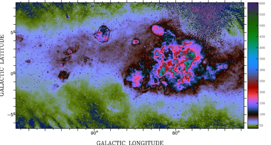
Figure 13 presents the survey data covering the Cygnus-X region and W 80 as a contour plot. We have used the same contour levels that were used in the previous best data on this area, the map published by Wendker et al. (1991). The resemblance to the earlier map is very strong; this is not surprising since the earlier data were also observed with the DRAO ST. The present data have better sensitivity by a factor of 4, superior removal of the effects of Cygnus A, and cover a larger area.

With the improved sensitivity of the present data, we see clearly the low-level envelope that surrounds the whole of Cygnus X (this is very evident in Figures 6 and 7, extending over the range of 65 ℓ 95). The emission here has thermal and non-thermal components. First, in the data of Reich & Reich (1988), spectral index between 408 and 1420 MHz at angular resolution~  , this region displays a0 . 9 lower temperature spectral index,b »2.4, than its surround-ings, whereb 2.6. Second, an extensive area of absorption is evident in the 22 MHz data of Roger et al. (1999), extending over at least 68 ℓ 90. It is likely that the thermal component of this emission lies at a distance of about 500 pc, the distance to the nearer parts of Cyg X and of W 80. The level of thermal emission here is much higher than at other points along the Galactic plane. The level of non-thermal emission behind Cygnus X at 408 MHz is about 60 K, judged by Figure 13. Cygnus X and W80. Alternating light and heavy contours are used. Contours are 60 K to 240 K in steps of 20 K, 240 K to 400 K in steps of 40 K, and 400 K to 800 K in steps of 100 K, 1000 K, and 1500 K. The 120 K contour is especially heavy.

10

Rygl et al. (2012)measured parallax distances to Cygnus-X objects, and place the entire complex at 1.400.08 kpc; their distance to W75N is 1.300.07kpc. However, Gottschalk et al. (2012)show that the molecular gas associated with W75N is definitely distinct from other molecular complexes.

16

comparing images from the present work with data from the Effelsberg 11-cm survey (Fürst et al.1990; Reich et al.1990a), using the technique illustrated in Section 7.3for the Perseus Arm (see Figure 14).

7.3. The Perseus Arm

The area around the HIIregions W3, W4, and W5 is shown in Figure14, where data from the present survey are compared to 2695 MHz data from Fürst et al. (1990) and Reich et al. (1990a). The 408 MHz image has been smoothed slightly to 4. 3¢ to match the angular resolution of the 2695 MHz data. The color scale for the figure has been chosen so that optically thin thermal emission has a very similar appearance in both images. Non-thermal objects will therefore stand out in the 408 MHz image; particularly evident are HB 3 (G132.7+0.3) and G127.1 +0.5, which are both well known SNRs.

The widespread low-level emission evident in the 408 MHz image at levels below about 40 K has no counterpart at 2695 MHz. If this was thermal emission, we would expect to see it at 2695 MHz at a level of ∼0.8 K, well above the

sensitivity limit of the 2695 MHz data. This is clearly non-thermal emission. Considering that it is well confined to low latitudes, most of it probably arises in the Perseus Arm. Similar extended emission, no doubt also non-thermal, is seen at

ℓ»150, where it reaches levels of 50 to 60 K (see Figure16).

7.4. Structures of Intermediate Size

Figure15presents a detailed look at a rich area containing a diversity of Galactic objects over a large range of distances. (i) HB21 (G89.0+4.7) is an SNR whose non-circular appearance indicates strong interaction with the ISM. Tatematsu et al. (1990)show that it is colliding with a molecular cloud on its eastern boundary; the distance to this molecular material, 0.8 kpc, establishes the distance to the SNR. (ii) CTB 104A (_{G93.7−0.2) is a similarly non-circular SNR, at a distance of} 1.5 kpc, that displays an unusual phenomenon: an HI shell surrounds CTB 104A and synchrotron emitting material has broken through the shell from the hot SNR interior, giving the SNR its distinctly non-circular appearance (Uyaniker et al.

2002). (iii) CTB 102 (G92.9+2.7), at a distance of 4.3 kpc, is an HII region and stellar wind bubble of size 100 to 130 pc (Arvidsson et al. 2009). (iv) The 408MHz emission from

BG2107+49 (G91.0+1.7) is thermal, but the source has a head–tail appearance, reminiscent of a radio galaxy. The tail traces the outline of a large, old stellar-wind bubble, while the head is a relatively young HII region (van der Werf & Higgs 1990), probably recently formed within the shell. The physical size of the bubble is 150 pc and the distance is ∼10 kpc. (v) NRAO655 (G93.4+1.8) and 3C 434.1 (G94.0 +1.0) are an HIIregion and SNR, respectively, but the two are at very similar distances (Foster & Routledge 2001; Foster et al. 2004) and may be parts of a larger complex. Newer distance estimates place the entire complex at 6.2 kpc, in the Figure 14. Area around the W3/W4/W5 complex at 408 MHz (top) and

2695 MHz (bottom). The angular resolution of both images is 4. 3¢ . The scales have been chosen so that optically thin thermal emission has the same appearance in both images. Note that the 2695 MHz image does not extend beyond- 5  b 5.

Figure 15. Area of 9 . 0 ´  centered at ℓ b9 . 0 (, )=(91 . 5, 1 . 9  ). The color scale is chosen to emphasize low-level extended emission. Contours are superimposed on parts of the image around some prominent objects mentioned in the text. Contour levels are 40 to 175 K in steps of 15 K, 175 to 295 K in steps of 30 K, and 295 to 505 K in steps of 70 K, 600, 720, and 840 K. The 85 K contour is white. Compact sources of sufficient intensity are white in the image, except where contours have been overlaid on them and they appear black.

17

Outer Arm of the Galaxy (T. Foster 2017, private communica-tion). (vi) Sharpless 2-124 (G94.6−1.5) is an HIIregion at a distance of 3.78 kpc (Foster & Brunt2015). The high angular resolution of this survey has enabled us to separate these objects in this crowded part of the sky.

At 408 MHz, among the sources of intermediate size, supernova remnants (SNRs) are dominant, more obvious than HIIregions. The excellent sensitivity of the survey to sources of synchrotron emission in the intermediate range of sizes is demonstrated in Figure16, showing an area of the Galactic plane in the second quadrant. This field is particularly rich in SNRs, and emission from seven SNRs is evident here. The brightest is HB9 (G160.9+2.6) and the faintest is G156.2+5.7, bright in X-rays (Pfeffermann et al. 1991) but extremely faint at radio wavelengths (Reich et al.1992). SNRs discovered from analyses of the data described here are also evident in Figure16, namely G151.2+2.9 (Kerton et al. 2007), G149.5+3.2, G150.5+3.8,

and G160.1−1.1 (Gerbrandt et al. 2014)_{, and G152.5−2.1} (Foster et al.2013). Other SNR discoveries in the CGPS data were reported by Kothes et al. (2001), Kothes (2003), Kothes et al. (2005), Tian et al. (2007), and Kothes et al. (2014). The key parameter in these discoveries has been spectral index, underlining the importance of a high-resolution survey at a low frequency. The power of low-frequency imaging with good angular resolution to discriminate between non-thermal and thermal emission is well illustrated by the work of Foster et al. (2006). These authors used the 408 MHz data, with other data, to show that OA 184 (G166.2+2.5), long classified as an SNR, is actually an HIIregion. Kothes et al. (2006)present a catalog of SNRs covering 70% of the CGPS area.

The other surveys listed in Table3 are invaluable resources in work like this, but the two CGPS surveys are crucial: they provide two surveys with high angular resolution with accurate depictions of extended emission. The CGPS 1420 MHz polarization data (Landecker et al.2010)have been especially valuable for recognition of SNR emission. Discovery and analysis of extended objects in the survey data have been accomplished by subtracting compact sources and smoothing the resulting map. This process is limited by source confusion, not thermal noise, as can be seen from a close inspection of Figure16.

8. Conclusions

We have described the execution and the data processing for a survey of the radio emission from the Galactic plane at 408 MHz. We have presented the survey images, and have given details of electronic access to them. Complete sampling of all spatial scales from the largest to the resolution limit (2. 8¢ ´ ¢ cosecδ) has been achieved by combining data from2. 8 aperture-synthesis and single-antenna telescopes. The image quality, especially the representation of extended structure, is extremely high. This is the only survey of the Galactic plane below 1 GHz that has arcminute resolution and faithful rendering of large structure. We have illustrated a number of uses of the survey data that exploit its good resolution; some allow us to reach conclusions about the extended emission. In particular, we have traced the warp in the synchrotron component of the disk in the outer Galaxy, and we have Table 3

Selected Surveys Covering the Northern Galactic Plane

Survey References F Beam Coverage Sens.

(MHz) ℓ _{b (mK)} DRAO-22 (1) 22 1°.1×1°.7a _{0° to 240°} Lb L CGPS 408 (2) 408 2 8a _{52° to 193°} −6°. 5 to 8°.5 760 CGPS 1420 (3) 1420 58″a _{52°.5 to 192°} −3°. 5 to 5°.5 60 Eff-21A (4) 1408 9 4 357° to 95°.5 −4° to 4° 40 Eff-21B (5) 1408 9 4 95°.5 to 240° −4° to 5° 30 Eff-11 (6), (7) 2695 4 3 358° to 240° −5° to 5° 17 Urumqi-A (8) 4800 9 5 10° to 60° −5° to 5° 1 Urumqi-B (9) 4800 9 5 60° to 129° −5° to 5° 0.9 Urumqi-C (10) 4800 9 5 129° to 230° −5° to 5° 0.6 Notes. a

Resolution is decl. dependent—see the references for details.

b

The 22 MHz survey covers −28°<δ<80° for all R.A.

References. (1) Roger et al. (1999); (2) this paper; (3) Taylor et al. (2003); (4) Reich et al. (1990b); (5) Reich et al. (1997); (6) Fürst et al. (1990); (7) Reich et al. (1990a); (8) Sun et al. (2011); (9) Xiao et al. (2011); (10) Gao et al (2010).

Figure 16. Area of 15 . 4 ´13 . 0 centered at ℓ b(, )=(154 . 9, 0 . 9  ). The color scale is chosen to emphasize low-level extended emission. Newly discovered SNRs G149.5+3.2, G150.5+3.8, G152.4−2.1, and G160.1−1.1 can be seen in this image. The very faint SNRs G156.2+5.7 and G151.2+2.9, as well as the bright SNR HB9 (G160.9+2.6) are also detectable here. Details of these objects are given in the text.

18

shown that the non-thermal contribution along the Galactic plane at 408 MHz amounts to ∼60 K at ℓ»80 and ∼40 K at ℓ»135.

We have established a flux density scale at 408 MHz by careful selection of calibration sources from three extensive source catalogs, the NVSS, the VLSS, and the 365 MHz Texas survey. This work supersedes previous attempts to calibrate the CGPS 408 MHz survey. The accuracy of flux densities is estimated to be 6%. The survey is partly limited by thermal noise, but also by source confusion. A complete catalog of small-diameter sources in the survey area will be presented in a future paper.

The contributions of many people underpin the work that we are privileged to report here: the entire CGPS team, at DRAO and in Canadian universities, played significant roles. We are grateful to Tyler Foster who provided valuable input on Galactic structure and distances to individual objects. We wish to record that Grote Reber contributed funds and encourage-ment to the realization of the 408 MHz channel on the Synthesis Telescope. The Dominion Radio Astrophysical Observatory is a National Facility operated by the National Research Council Canada. The Canadian Galactic Plane Survey is a Canadian project with international partners, and is supported by the Natural Sciences and Engineering Research Council (NSERC).

ORCID iDs

R. Kothes https://orcid.org/0000-0001-5953-0100

References

Armond, T., Reipurth, B., Bally, J., & Aspin, C. 2011,A&A,528, A125

Arvidsson, K., Kerton, C. R., & Foster, T. 2009,ApJ,700, 1000

Baars, J. W. M., Genzel, R., Pauliny-Toth, I. I. K., & Witzel, A. 1977, A&A,

61, 99

Binney, J., & Merrifield, M. 1998, Galactic Astronomy (Princeton, NJ: Princeton Univ. Press)

Cohen, A. S., Lane, W. M., Cotton, W. D., et al. 2007,AJ,134, 1245

Comerón, F., & Pasquali, A. 2005,A&A,430, 541

Condon, J. J. 2002, in ASP Conf. Ser. 278, Single-Dish Radio Astronomy: Techniques and Applications, ed. S. Stanimirovic et al. (San Francisco, CA: ASP),155

Condon, J. J., Cotton, W. D., Greisen, E. W., et al. 1998,AJ,115, 1693

Douglas, J. N., Bash, F. N., Bozyan, F. A., Torrence, G. W., & Wolfe, C. 1996, AJ,111, 1945

Feldt, C. 1993, A&A,276, 531

Feldt, C., & Wendker, H. J. 1993, A&AS,100, 287

Fich, M., & Blitz, L. 1984,ApJ,279, 125

Foster, T., & Brunt, C. M. 2015,AJ,150, 147

Foster, T., Kothes, R., Sun, X. H., Reich, W., & Han, J. L. 2006,A&A,454, 517

Foster, T., & Routledge, D. 2001,A&A,367, 635

Foster, T., Routledge, D., & Kothes, R. 2004,A&A,417, 79

Foster, T. J., Cooper, B., Reich, W., Kothes, R., & West, J. 2013,A&A,

549, A107

Fürst, E., Reich, W., Reich, P., & Reif, K. 1990, A&AS,85, 691

Gao, X. Y., Reich, W., Han, J. L., et al. 2010,A&A,515, A64

Gerbrandt, S., Foster, T. J., Kothes, R., Geisbüsch, J., & Tung, A. 2014,A&A,

566, A76

Gottschalk, M., Kothes, R., Matthews, H. E., Landecker, T. L., & Dent, W. R. F. 2012,A&A,541, A79

Hales, S. E. G., Riley, J. M., Waldram, E. M., Warner, P. J., & Baldwin, J. E. 2007,MNRAS,382, 1639

Haslam, C. G. T., Salter, C. J., Stoffel, H., & Wilson, W. E. 1982, A&AS,47, 1

Higgs, L. A., Hoffmann, A. P., & Willis, A. G. 1997, in ASP Conf. Ser. 125, Astronomical Data Analysis Software and Systems VI, ed. G. Hunt & H. Payne (San Francisco, CA: ASP),58

Higgs, L. A., Landecker, T. L., & Roger, R. S. 1977,AJ,82, 718

Kass, R. E., & Raftery, A. E. 1995,J. Am. Stat. Assoc., 90, 773 Kerton, C. R., Murphy, J., & Patterson, J. 2007,MNRAS,379, 289

Knödlseder, J. 2000, A&A,360, 539

Knödlseder, J. 2004, arXiv:astro-ph/0407050

Kothes, R. 2003,A&A,408, 187

Kothes, R., Fedotov, K., Foster, T. J., & Uyanıker, B. 2006,A&A,457, 1081

Kothes, R., Landecker, T. L., Foster, T., & Leahy, D. A. 2001,A&A,376, 641

Kothes, R., Sun, X. H., Reich, W., & Foster, T. J. 2014,ApJL,784, L26

Kothes, R., Uyanıker, B., & Reid, R. I. 2005,A&A,444, 871

Landecker, T. L., Dewdney, P. E., Burgess, T. A., et al. 2000,A&AS,145, 509

Landecker, T. L., Reich, W., Reid, R. I., et al. 2010,A&A,520, A80

Laugalys, V., Straižys, V., Vrba, F. J., et al. 2006, BaltA,15, 483

Lo, W. F., Dewdney, P. E., Landecker, T. L., Routledge, D., & Vaneldik, J. F. 1984,RaSc,19, 1413

Lynds, B. T. 1962,ApJS,7, 1

Pauliny-Toth, I. K., & Shakeshaft, J. R. 1962,MNRAS,124, 61

Perley, R. A., & Butler, B. J. 2013,ApJS,206, 16

Perley, R. A., & Butler, B. J. 2017,ApJS,230, 7

Pfeffermann, E., Aschenbach, B., & Predehl, P. 1991, A&A,246, L28

Reich, P., & Reich, W. 1988, A&AS,74, 7

Reich, P., Reich, W., & Furst, E. 1997,A&AS,126, 413

Reich, W., Fuerst, E., & Arnal, E. M. 1992, A&A,256, 214

Reich, W., Fuerst, E., Reich, P., & Reif, K. 1990a, A&AS,85, 633

Reich, W., Reich, P., & Fuerst, E. 1990b, A&AS,83, 539

Remazeilles, M., Dickinson, C., Banday, A. J., Bigot-Sazy, M.-A., & Ghosh, T. 2015,MNRAS,451, 4311

Rengelink, R. B., Tang, Y., de Bruyn, A. G., et al. 1997,A&AS,124, 259

Roger, R. S., Costain, C. H., & Bridle, A. H. 1973,AJ,78, 1030

Roger, R. S., Costain, C. H., Landecker, T. L., & Swerdlyk, C. M. 1999, A&AS,137, 7

Rygl, K. L. J., Brunthaler, A., Sanna, A., et al. 2012,A&A,539, A79

Sun, X. H., Reich, W., Han, J. L., et al. 2011,A&A,527, A74

Tatematsu, K., Fukui, Y., Landecker, T. L., & Roger, R. S. 1990, A&A,237, 189

Taylor, A. R., Gibson, S. J., Peracaula, M., et al. 2003,AJ,125, 3145

Tian, W. W., Leahy, D. A., & Foster, T. J. 2007,A&A,465, 907

Uyaniker, B., Kothes, R., & Brunt, C. M. 2002,ApJ,565, 1022

van der Werf, P. P., & Higgs, L. A. 1990, A&A,235, 407

Veidt, B. G., Landecker, T. L., Dewdney, P. E., Vaneldik, J. F., & Routledge, D. 1985,RaSc,20, 1118

Vessey, S. J., & Green, D. A. 1998,MNRAS,294, 607

Wendker, H. J., Higgs, L. A., & Landecker, T. L. 1991, A&A,241, 551

Westerhout, G. 1958, BAN,14, 215

Willis, A. G. 1999,A&AS,136, 603

Xiao, L., Han, J. L., Reich, W., et al. 2011,A&A,529, A15

19