Collinearity isn't a disease that needs curing

https://doi.org/10.15626/MP.2021.2548 Article type: Commentary

Published under the CC-BY4.0 license

Open materials: Yes Open and reproducible analysis: Yes Open reviews and editorial process: Yes

Preregistration: Not applicable

Reviewed by: N. Brown & J. Ferreira Analysis reproduced by: André Kalmendal All supplementary files can be accessed at OSF: https://doi.org/10.17605/OSF.IO/72GAC

Collinearity isn’t a disease that needs curing

Jan Vanhove

University of Fribourg

Abstract

Once they have learnt about the effects of collinearity on the output of multiple regression models, researchers may unduly worry about these and resort to (sometimes dubious) modelling techniques to mitigate them. I argue that, to the extent that problems occur in the presence of collinearity, they are not caused by it but rather by common mental shortcuts that researchers take when interpreting statistical models and that can also lead them astray in the absence of collinearity. Moreover, I illustrate that common strategies for dealing with collinearity only sidestep the perceived problem by biasing parameter estimates, reformulating the model in such a way that it maps onto different research questions, or both. I conclude that collinearity in itself is not a problem and that researchers should be aware of what their approaches for addressing it actually achieve.

Keywords: regression assumptions, multiple regression, interpreting regression models As researchers and students learn more about

statisti-cal models, they sooner or later stumble across the term (multi)collinearity. Collinearity, which roughly means that the predictors in a statistical model are correlated with each other, is often cast as a problem for statis-tical analysis. This suggests that the conscientious an-alyst has to solve it. I will argue that, to the extent that problems occur in the presence of collinearity, these are not caused by the collinearity itself but rather by a faulty way of thinking about statistical models that can lead analysts astray even in the absence of collinear-ity. Common strategies for dealing with collinear predic-tors do not solve these perceived problems but instead sidestep them, often by fitting a model that, perhaps unbeknownst to the analyst, answers a different set of questions from the original one.

This article does not present any novel insights, but I hope that it will nonetheless be educational to read-ers who sometimes find the output of regression mod-els befuddling. I will focus on collinearity between two continuous predictors in (ordinary least squares) mul-tiple regression models. In this case the strength of the collinearity can be gauged from the correlation be-tween the predictors. However, all of my points apply

to models with categorical predictors or a mix of cat-egorical and continuous predictors as well. I will not discuss methods for assessing the degree of collinearity between three or more predictors for the simple reason that I find them a distraction: in what follows, I will argue that collinearity is not a statistical problem and should not be checked for (also see O’Brien,2007).

Collinearity and its consequences

Collinearity means that a substantial amount of in-formation contained in some of the predictors included in a statistical model can be pieced together as a lin-ear combination of some of the other predictors in the model. The easiest case is when you have a multiple linear regression model with two correlated predictors, as in the examples to follow. These predictors can be continuous or categorical, but I will stick to continuous predictors for ease of exposition.

I created four datasets with two continuous predic-tors to illustrate collinearity and its consequences. You can find the R code to reproduce all analyses at https: //osf.io/jupd8/. The outcome in each dataset was cre-ated using the following equation; the parameter values

were chosen arbitrarily:

outcomei= 0.4 × predictor1i+ 1.9 × predictor2i+ εi,

(1) where the residuals (εi) were drawn from a normal

dis-tribution with a standard deviation of 3.5.1

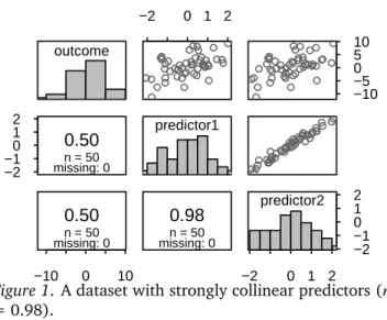
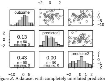
The four datasets are presented in Figures1through 4. In Figure1, a linear function of predictor1 captures most of the information contained in predictor2, so the two predictors are strongly collinear. In Figure 3, by contrast, both predictors are completely unrelated, and a linear function of one predictor cannot capture any information in the other. Hence, the two predic-tors are not collinear at all. Some readers may be sur-prised to see that I consider a situation where two pre-dictors are correlated at r = 0.50 (Figure 2) to be a case of weak rather than moderate or strong collinear-ity. But in fact, the consequences of having two pre-dictors that are correlated at r = 0.50 (rather than at r = 0.00) are negligible. Finally, Figure 4 highlights the linear part in collinearity: while the two predictors in this figure are related in that predictor2 perfectly determines predictor1, there is no linear relationship between them whatsoever. (You cannot uniquely de-termine the value for predictor2 when you know the value for predictor1, though.) The dataset in Figure 4is not affected by any of the statistical consequences of collinearity, but it will be useful to illustrate a point I want to make below.

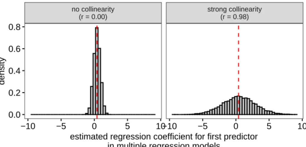
To illustrate the statistical consequences of collinear-ity, I simulated 10,000 samples of 50 observations in which the two predictors were highly correlated (sam-ple correlation of r = 0.98, yielding datasets similar to the one in Figure1) and 10,000 samples of 50 observa-tions in which they were completely orthogonal (sam-ple r = 0.00, yielding datasets similar to the one in Figure3). In all cases, both predictors were indepen-dently related to the outcome according to Equation 1. On each simulated sample, I ran a multiple regression model from which I extracted the estimated model co-efficients. Figure5shows the estimated coefficients for the first predictor, whose true parameter value is 0.4. Clearly, the estimates vary more when the predictors are strongly correlated than when they are not, such that individual estimates can lie farther from the true parameter value and often have the opposite sign from this true parameter value. However, on average, the estimates equal the true parameter value. In statistics parlance, they are “unbiased.”

Crucially, and happily, this greater variability is re-flected in the standard errors and confidence intervals around these estimates: The standard errors and con-fidence intervals are automatically wider when the es-timated coefficients are affected by collinearity. This is

outcome −2 −10 1 2

0.50

n = 50 missing: 0 −10 0 10

0.50

n = 50 missing: 0 −2 0 1 2 predictor1

0.98

n = 50 missing: 0 −10 −5 0 5 10 −2 0 1 2 −2 −1 0 1 2 predictor2

Figure 1. A dataset with strongly collinear predictors (r = 0.98).

illustrated in Figure6: If you fit multiple regressions on the datasets plotted in Figures 1 to 4, the confidence intervals are considerably wider if the predictors are strongly collinear than when they are not. Moreover, the confidence intervals retain their nominal coverage rates (i.e., x% of the x% confidence intervals contain the true parameter value). So the statistical consequence of collinearity is automatically taken care of in the model’s output and requires no additional computations on the part of the analyst.

The greater variability in the estimates, and the ap-propriately larger standard errors and wider confidence intervals all reflect a relative lack of information in the sample (also see Morrissey and Ruxton,2018). It is dif-ficult to improve on York’s (2012) explanation of the problem and possible solutions:

“Collinearity is at base a problem about in-formation. If two factors are highly corre-lated, researchers do not have ready access 1_{Some researchers examining the consequences of} collinearity generate both the predictors and the outcome di-rectly from multivariate normal distributions in which the cor-relation between the predictors varies but the corcor-relations be-tween the outcome and the individual predictors do not (e.g., Wurm and Fisicaro,2014) rather than generating the outcome as a function of the predictors as I did. In doing so, they im-plicitly allow the true regression equation to vary from sim-ulation to simsim-ulation: If you fix the correlations between the predictors and the outcome, but you want to vary the inter-correlation between the predictors, you have to vary the β parameters (fixed at 0.4 and 1.9 in my example) and the σ parameter (fixed at 3.5 in my example). The result of this is that such simulations may paradoxically show that you obtain

more significant estimates when the predictors are strongly

collinear (see Wurm and Fisicaro, 2014, Table 6), but they actually compare different data generating processes.

outcome −2 0 2

0.31

n = 50 missing: 0 −10 0 5

0.46

n = 50 missing: 0 −2 0 2 predictor1

0.50

n = 50 missing: 0 −10 −5 0 5 −2 0 2 −2 0 2 predictor2

Figure 2. A dataset with weakly collinear predictors (r = 0.50). outcome −2 0 2

0.13

n = 50 missing: 0 −10 0 5

0.43

n = 50 missing: 0 −2 0 2 predictor1

0.00

n = 50 missing: 0 −10 −5 0 5 −2 0 1 2 −2 −1 0 1 2 predictor2

Figure 3. A dataset with completely unrelated predictors (r = 0.00). outcome −1.5 −0.5 0.5 1.5 0.15 n = 50 missing: 0 −5 0 5 0.52 n = 50 missing: 0 −1.5 0.0 1.5 predictor1 0.00 n = 50 missing: 0 −5 0 5 −1.5 0.0 1.5 −1.5 −0.5 0.5 1.5 predictor2

Figure 4. A dataset with orthogonal (r= 0.00) but per-fectly related predictors: Once you know the value of predictor2, you know the value of predictor1.

to much information about conditions of the dependent variables when only one of the factors actually varies and the other does not. If we are faced with this problem, there are really only three fundamental solutions: (1) find or create (e.g. via an experimen-tal design) circumstances where there is re-duced collinearity; (2) get more data (i.e. in-crease the N size), so that there is a greater quantity of information about rare instances where there is some divergence between the collinear variables; or (3) add a variable or variables to the model, with some degree of independence from the other independent variables, that explain(s) more of the vari-ance of Y, so that there is more informa-tion about that which is being modeled.” (p. 1384)

Is collinearity a problem?

For the most part, I think that collinearity is a prob-lem for statistical analyses in the same way that Bel-gium’s lack of mountains is detrimental to the country’s chances of hosting the Winter Olympics: It is an un-fortunate fact of life, but not something that has to be solved. The three solutions that York (2012) mentions, i.e., running another study, obtaining more data or re-ducing the error variance using covariates, are all sensi-ble, but if you have to work with the data that you have, the model output will be unbiased and will appropri-ately reflect the degree of uncertainty in the estimates.

So I do not consider collinearity a problem. What is the case, however, is that collinearity highlights prob-lems with the way many people think about statistical models and inferential statistics. Let’s look at a couple of these.

“Collinearity decreases statistical power.”

You may have heard that collinearity decreases sta-tistical power, i.e., the chances of obtaining a statisti-cally significant coefficient estimate if the true param-eter value is different from zero. This is true, but the lower statistical power is a direct result of the larger standard errors, which appropriately reflect the greater sampling variability of the estimates. This is only a problem if you interpret “lack of statistical significance” as “zero effect.” But then the problem does not lie with collinearity but with the belief that non-significant estimates indicate zero effects. (Schmidt (1996) calls this false belief “the most devastating of all to the re-search enterprise” (p. 126).) It is just that this false belief is even more likely than usual to lead you astray

no collinearity (r = 0.00) strong collinearity (r = 0.98) −10 −5 0 5 10−10 −5 0 5 10 0.0 0.2 0.4 0.6 0.8

estimated regression coefficient for first predictor in multiple regression models

density

Figure 5. The parameters for the first predictor in 10,000 samples as estimated by multiple linear regression models. When the predictors are strongly collinear, the estimates vary more from sample to sample, but the estimates are unbiased in either case. The dashed vertical lines show the true parameter value (0.4).

(Intercept) predictor1 predictor2

−1 0 1 −2.5 0.0 2.5 5.0 −2.5 0.0 2.5 5.0 no collinearity (related predictors) no collinearity (unrelated predictors) weak collinearity strong collinearity

estimated coefficient with 95% confidence interval

Figure 6. Estimated coefficients and their 95% confidence intervals for the models fitted to the four datasets. The dashed vertical lines show the true parameter values.

when your predictors are collinear. If instead of focus-ing solely on the p-value, you take into account both the estimate and its uncertainty interval, then there is no problem.

Incidentally, I think that some people may be misled when they hear that collinearity “decreases” statistical power or “increases” standard errors as this wording may be taken to suggest that collinearity is a process that can be halted or reversed. It is true that compared to situations in which there is less or no collinearity and all other things are equal, the standard errors are larger and statistical power is lower when there is stronger collinearity. But outside of computer simulations, you cannot reduce collinearity while keeping all other things equal. In the real world, collinearity is not an unfolding process that can be nipped in the bud without bringing about other changes in the research design, the sam-pling procedure, or the statistical model and its inter-pretation.

Similarly, you may have heard that collinearity “in-flates” standard errors or p-values. This wording, too,

is misleading as it suggests that, in the presence of collinearity, standard errors and p-values are larger than they should have been. They are not, as per the discus-sion in the previous section (see Morrissey and Ruxton, 2018).

“None of the predictors is significant but the overall model fit is.”

With collinear predictors, you may end up with a sta-tistical model for which the F-test of the overall model fit is highly significant but that does not contain a single significant predictor. This is illustrated in Table1. The overall model fit for the dataset with strong collinear-ity (see Figure1) is highly significant, but as shown in Figure6, neither predictor has an estimated coefficient that is significantly different from zero: Both 95% con-fidence intervals contain zero.

If this seems strange, you need to keep in mind that the tests for the individual coefficient estimates and the test for the overall model fit seek to answer different

Table 1

F-tests and p-values for the overall model fit for the multiple regression models on the four datasets. Even though neither predictor has a significant estimated coefficient in the ‘strong collinearity’ dataset (as shown in Figure 6), the overall fit is highly significant.

Dataset F-test p-value

strong collinearity F(3, 47) = 8.0 0.001

weak collinearity F(3, 47) = 6.6 0.003

no collinearity (unrelated predictors) F(3, 47) = 5.9 0.005

no collinearity (related predictors) F(3, 47) = 9.8 0.000

questions, so there is no contradiction if they yield dif-ferent answers. To elaborate, the test for the overall model fit asks if all predictors jointly can account for variance in the outcome; the tests for the individual coefficients ask whether these are different from zero. With collinear predictors, it is possible that the answer to the first question is “yes” and the answer to the sec-ond is “I have no idea.” The reason for this is that with collinear predictors, either predictor could act as the stand-in of the other so that, as far as the model is concerned, either coefficient could well be zero, as long as the other is not. But due to the lack of information in the collinear sample, it is not sure which, if any, is zero (see McElreath,2020, Chapter 6, for a lucid expla-nation).

So again, there is no real problem: The tests answer different questions, so they may yield different answers. It is just that when you have collinear predictors, this tends to happen more often than when you do not.

“Collinearity means that you can’t take model coef-ficients at face value.”

It is sometimes said that collinearity makes it more difficult to interpret estimated model coefficients. But the appropriate interpretation of an estimated regres-sion coefficient is always the same, regardless of the degree of collinearity: According to the model, what would the difference in the mean outcome be if you took two large groups of observations that differed by one unit in the focal predictor but whose other predic-tor values were the same. The emphasised clause is cru-cial, and note the absence of any appeal to causality in the previous sentence. The interpretational difficulties that become obvious when there is collinearity are not caused by the collinearity itself but by mental shortcuts that people take when interpreting regression models.

For instance, you may obtain a coefficient estimate in a multiple regression model with collinear predictors that you interpret to mean that older children perform more poorly on a foreign-language (L2) writing task than younger children. This would be counterintuitive, and you may find that, in your sample, older children

actually outperform younger ones. You could chalk this one up to collinearity, but the problem really is related to a faulty mental shortcut you took when interpreting your model: You forgot to take into account the crucial “but whose other predictor values are the same” clause. If your model also includes measures of the children’s previous exposure to the L2, their motivation to learn the L2, and their L2 vocabulary knowledge, then what the estimated coefficient means is emphatically not that, according to the model, older children perform on av-erage more poorly on a writing task than younger chil-dren. What it means is that, according to the model, older children perform more poorly than younger chil-dren with the same values on the previous exposure, mo-tivation, and vocabulary knowledge measures. If, on re-flection, this is not what you are actually interested in, then you should fit a different model (also see Miller and Chapman, 2001, for a similar point in the context of analysis of covariance). For instance, if you are in-terested in the overall difference between younger and older children regardless of their previous exposure, motivation and vocabulary knowledge, do not include these variables as predictors. But then you should have also not included these predictors if the collinearity had not been as strong.

Another interpretational difficulty emerges if you re-cast the interpretation of the estimate as follows: Ac-cording to the model, what would the expected differ-ence in mean outcome be if you took an observation and increased its value on the focal predictor by one unit but kept the other predictor values constant? The difference between this interpretation and the one that I offered earlier is that we have moved from a purely descriptive one to both a causal and an interventionist one (viz., the idea that one could change some predictor values while keeping the others constant and that this would have an effect on the outcome). In the face of strong collinear-ity, it becomes clear that this interventionist interpreta-tion may be wishful thinking: It may be impossible to change values in one predictor without also changing values in the predictors that are collinear with it. But the problem here again is not the collinearity but the mental shortcut in the interpretation. Statistical models

describe associations; imbuing them with a causal or even interventionist interpretation requires strong ad-ditional assumptions (for guidance, see Elwert, 2013; Rohrer,2018; Shmueli,2010).

In fact, you can run into the same difficulties when you apply the interventionist mental shortcut in the ab-sence of collinearity: In the dataset shown in Figure4, it is impossible to change the second predictor without also changing the first since the first is a transformation of the second. Yet the two variables are not collinear, since the transformation is completely nonlinear. Or say you want to model quality ratings of texts in terms of the number of words in the text (“tokens”), the number of unique words in the text (“types”), and the type/to-ken ratio. The model will output estimated coefficients for the three predictors, but as an analyst you should realise that it is impossible to find two texts differing in the number of tokens but having both the same number of types and the same type/token ratio: If you change the number of tokens and keep constant the number of types, the type/token ratio changes, too.

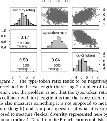
A final mental shortcut that is laid bare in the pres-ence of collinearity is conflating a measured variable with the theoretical construct that this variable is as-sumed to capture. Conflating measurements and con-structs can completely invalidate the conclusions drawn from a model even in the absence of collinearity (see Berthele and Vanhove,2020; Brunner and Austin,2009; Loftus, 1978; Wagenmakers et al., 2012; Westfall and Yarkoni,2016). The literature on lexical diversity offers another case in point. The type/token ratio (TTR) dis-cussed in the previous paragraph is one of several pos-sible measures of a text’s lexical diversity. If you take a collection of otherwise comparable texts, chances are that the longer texts tend to have lower TTR values (see Malvern et al.,2004, Chapter 2). This text-size depen-dence has led quantitative linguists to abandon the use of the TTR, even though the relationship in any given dataset need not be that strong (see Figure7for an ex-ample).

However, the reason why researchers have aban-doned the use of the TTR is not collinearity per se. Rather, it is that the TTR is a poor measure of what it is supposed to capture, viz., the lexical diversity dis-played in a text. Specifically, because of the statistical properties of language, the TTR is pretty much bound to conflate a text’s lexical diversity with its length. The negative correlation between the TTR and text length is not a big problem for statistical modelling, but it is a symptom of a more fundamental problem: A measure of lexical diversity should not as a matter of fact be re-lated to text length. The fact that the TTR is shows that it is a poor measure of lexical diversity. This problem

diversity rating 0.4 0.6 0.8 1.0 −0.17 n = 1000 missing: 0 2 4 6 8 0.58 n = 1000 missing: 0 0.4 0.6 0.8 1.0 type/token ratio −0.66 n = 1000 missing: 0 2 4 6 8 4 5 6 7 8 4 5 6 7 8 log−2 tokens

Figure 7. The type/token ratio tends to be negatively correlated with text length (here: log-2 number of to-kens). But the problem is not that the type/token ratio is collinear with text length; it is that the type/token ra-tio also measures something it is not supposed to mea-sure (length) and is a poor meamea-sure of what it is sup-posed to measure (lexical diversity, represented here by human ratings). Data from the French corpus published by Vanhove et al.,2019.

is hidden if researchers mentally equate the TTR with the construct of lexical diversity rather than remaining cognizant of the fact that it is but an attempt to quantify the construct—and not a successful one at that.

To be clear, it is not necessarily a problem that mea-sures of lexical diversity empirically correlate with text length. After all, it is possible that the lexical diversity of longer texts is greater than that of shorter texts or vice versa: Texts may be pithy but lexically diverse if the writers often used le mot juste instead of elaborate cir-cumlocutions, and long texts may be lexically more di-verse than shorter ones if they were written by more so-phisticated writers with more to tell. The problem with the TTR is that it almost necessarily correlates with text length, even if, at the construct level, the texts’ lexical diversity does not. For instance, if you take increasingly longer snippets of texts from the same book, you will find that the TTR goes down (see Tweedie and Baayen, 1998). This does not mean that the writer’s vocabulary skills went down in the process of writing the book, but that s/he had to reuse common words (e.g., articles, pronouns, prepositions, copula verbs, common or im-portant content words). More generally, if your predic-tors correlate strongly when they are not supposed to, your problem is not collinearity, but it may be that in trying to capture one construct, you have also captured the one represented by the other predictor.

when predictors are collinear are not caused by the collinearity itself but by mental shortcuts that may lead researchers astray even in the absence of collinearity.

Collinearity does not require a statistical solution

I have argued that collinearity is not a genuine statis-tical problem, so I do not think it should be addressed by statistical means. Let’s take a closer look at some pop-ular strategies that analysts resort to when their predic-tors are collinear and the repercussions of these strate-gies.

Residualising predictors

The first popular strategy for dealing with collinear-ity is to residualise one collinear predictor against the other. This means that one of the predictors is fitted as the dependent variable in a regression model with the other predictor(s) as the independent variable(s). The estimated residuals are extracted from this model and then used as a replacement for the original predictor in the multiple regression model. York (2012) and Wurm and Fisicaro (2014) comprehensively discuss the conse-quences of this approach; Figure8highlights the main points.

As seen in the top left and bottom right panels, resid-ualising one of the predictors against the other and us-ing these residuals in lieu of the original predictor does not bias the estimates for the residualised predictor rel-ative to the original true parameter values in Equation (1). It also does not reduce the sample-to-sample vari-ability of these estimates. So, as far as the residualised predictor is concerned, there is no downside or upside to this approach. However, as seen in the top right and bottom left panels, the estimates of the residualiser (i.e., the predictor that was not residualised) show less sample-to-sample variability, but they are substantially biased relative to the original true parameter values in Equation (1) when the original predictors are collinear.2 The reason for this is that any variance in the outcome that could be accounted for by both predictors is now assigned wholly to the residualiser (see York,2012).

Residualising one of the predictors against the other, then, changes the meaning of the estimated coefficient for the residualiser in a way that I suspect is opaque to most analysts and consumers. In fact, I cannot wrap my head around the sentence that I am about to foist upon you: What, according to the model, would be the mean difference if you took a large group of data points that differed by one unit in the residualiser but whose other predictor values differed by the same amount and in the same direction from the values that you would expect this predictor to have based on the linear asso-ciation between it and the residualiser in the sample?

(Everything following but describes what it means for the estimated residuals to be held constant.) Perhaps such estimates can be useful, but hardly more than once in a blue moon.

Dropping collinear predictors

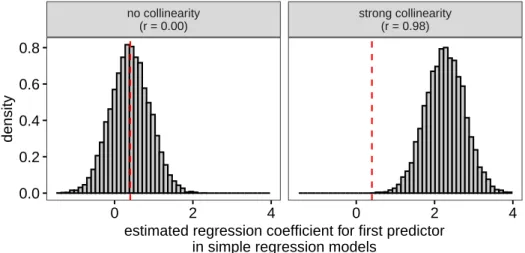
A second approach is to drop one or more of the collinear predictors from the model. I have no prob-lem with this approach per se. But the probprob-lem that it solves is not collinearity but rather that the original model was misspecified. This approach only represents a solution if the new model is capable of answering the research question since, crucially, estimated coefficients from models with different predictors do not have the same meaning.

For instance, say you are interested in the associa-tion between L2 grammatical knowledge and L2 read-ing proficiency and you fit a model with L2 readread-ing test scores as the outcome, the learners’ scores on an L2 grammar test as the focal predictor and their scores on an L2 vocabulary test as a ‘control variable.’ If you decide to drop the vocabulary test scores from the model because of their correlation with the grammar test scores, you change the meaning of the estimate of the coefficient for the grammar test scores. In the full model, this estimate captures the mean difference in reading proficiency between learners with the same vocabulary score but with a one-unit difference in gram-mar test scores. In the reduced model, the estimate captures the mean difference in reading proficiency be-tween learners with a one-unit difference in grammar test scores, regardless of their performance on the vo-cabulary test score. Either estimate may be useful for addressing the research question, but this depends on the research question, not on the degree of collinearity. If the reduced model makes more sense than the full model in the presence of collinearity, it would have also made more sense in the absence of collinearity.

Something to be particularly aware of is that by drop-ping one of the collinear predictors, you bias the esti-mates of the other predictors relative to their original parameter values as shown in Figure9(and see Note 2). The reason is that, thanks to their correlation with the dropped predictor, the remaining predictors can now do some of its job in accounting for variance in the out-come.

2_{I say “relative to the original true parameter values” since,} technically, the estimates in the new model are not biased ei-ther, but they estimate something different from the estimates in the original model.

predictor1 predictor2 predictor1 residualised predictor2 residualised −10 −5 0 5 10 −5 0 5 10 0.0 0.2 0.4 0.6 0.8 0.0 0.2 0.4 0.6 0.8

estimated regression coefficients for the predictors in multiple regression models

after one of them has been residualised against the other

density

Figure 8. In the presence of strong collinearity (r= 0.98), residualising one of the predictors against the other does not bias the estimates for the residualised predictor or reduce their sample-to-sample variability (top left and bottom right), but it does bias the estimates of the residualiser (top right and bottom left) relative to the original parameter values (shown as dashed vertical lines).

no collinearity (r = 0.00) strong collinearity (r = 0.98) 0 2 4 0 2 4 0.0 0.2 0.4 0.6 0.8

estimated regression coefficient for first predictor in simple regression models

density

Figure 9. Dropping a collinear predictor changes the meaning of the estimate for the predictor retained (right panel). The reduced model now yields biased estimates of the original parameters (represented by the dashed vertical lines). When the predictors are perfectly orthogonal, this does not happen, but this is a special case.

Averaging predictors

A third strategy for dealing with collinearity is to compress the information in the collinear predictors into a smaller set of less strongly correlated predictors. For instance, analysts sometimes take the average of several (possibly z-standardised) predictors and use this average instead of the original predictors. Alternatively, they might submit these predictors to a principal ponent or factor analysis and extract one or more

com-ponents or factors from this analysis to use these in lieu of the original predictors.

I do not mind this approach per se, either, but ana-lysts should be aware that the meaning of their model estimates is now different from those in the model that they originally fitted. The estimates now express the model’s best guess of the mean difference in the out-come when sampling a large number of data points that differ in one unit in the newly created variable but have

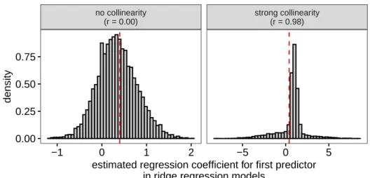
no collinearity (r = 0.00) strong collinearity (r = 0.98) −1 0 1 2 −5 0 5 0.00 0.25 0.50 0.75

estimated regression coefficient for first predictor in ridge regression models

density

Figure 10. Ridge regression is a form of biased estimation, so naturally the estimates it yields are biased. When the predictors are orthogonal, all estimates are biased towards zero (left panel). When the predictors are collinear, the estimates for the weaker predictor are biased away from zero (right panel), whereas the estimates for the stronger predictor are biased towards zero (not shown).

otherwise identical predictor variables. Depending on the research question, such a model may be more defensible than the model originally fitted. But this de-pends on the research question, not on the degree of collinearity between the predictors.

Using estimation methods such as ridge regression

With independently and identically distributed errors (i.e., when the independence and homoskedasticity as-sumptions are met), ordinary least squares regression is guaranteed to yield unbiased estimates with the lowest possible sample-to-sample variability. Ridge regression and its cousins (lasso, elastic net) sacrifice unbiased-ness in order to obtain estimates with an even lower sample-to-sample variability. This can be particularly useful in models optimised for predicting (as opposed to describing or explaining; see Kuhn and Johnson,2013; Shmueli, 2010). Since collinearity is associated with more variable estimates, it is understandable that ridge regression and the like are used to tackle it. But the result of using models that deliberately bias the esti-mates is, quite naturally, that you end up with biased estimates.

I illustrate this in Figure10, for which I reanalysed the data underlying Figure 5 using ridge regression. (Details of the choice of the λ parameter are available in the supplementary materials, but they are not impor-tant here.) For orthogonal predictors, all estimates are biased towards zero. For strongly collinear predictors, the estimates for the weaker predictor will be biased away from zero (shown in the figure), and those for the stronger predictor will be biased towards zero.

Biased estimation, then, reduces sampling variability

in the estimates, but at the cost of, well, biased estima-tion. Moreover, the usefulness of standard errors and confidence intervals for ridge regressions and its cousins is contested (see Goeman et al., 2018), so a further drawback is debatable statistical inference.3

In sum, popular strategies to address collinearity in-volve giving up the unbiased estimates of ordinary least squares regression, redefining the statistical model so that it answers different questions from the original model, or both. As York (2012) writes,

“Statistical ‘solutions,’ such as residualiza-tion that are often used to address collinear-ity problems do not, in fact, address the fun-damental issue, a limited quantity of infor-mation, but rather serve to obfuscate it. It is perhaps obvious to point out, but nonethe-less important in light of the widespread confusion on the matter, that no statistical procedure can actually produce more infor-mation than exists in the data.” [p. 1384]

Summary

Collinearity is a form of lack of information that is already appropriately reflected in the output of your statistical model. When collinearity is associated with 3_{With informative prior distributions on the parameters,} Bayesian models can yield fairly narrow posterior distribu-tions (i.e., a fairly low degree of uncertainty) for the estimates even in the presence of collinearity. But this is achieved by virtue of incorporating information from outside the sample into the model by means of the prior distributions, not by con-juring information out of thin air.

interpretational difficulties, these difficulties are not caused by the collinearity itself. Rather, they reveal that the model was poorly specified (in that it answers a question different from the one of interest), that the analyst has overly focused on significance rather than estimates and the uncertainty about them, or that the analyst took a mental shortcut in interpreting the model that could have also led them astray in the absence of collinearity. These shortcuts include failing to interpret parameter estimates conditional on all the other predic-tors in the model, lending a causal or interventionist interpretation to what is a descriptive model without proper justification, and conflating a measure with the construct that it is supposed to represent. Lastly, if you do decide to deal with collinearity, make sure you can still answer the question of interest and that any bias in the estimates can be justified.

Author Contact

Jan Vanhove, University of Fribourg, Department

of Multilingualism, Rue de Rome 1, 1700

Fri-bourg, Switzerland. ORCID ID: https://orcid.org/

0000-0002-4607-4836. Website: https://janhove.

github.io.

I thank Twitter user @facupalacio12 for the reference to Morrissey and Ruxton (2018), and Johan Ferreira, Nick Brown, and Rickard Carlsson for their comments.

Conflict of Interest and Funding

The author declares no conflict of interest and did receive specific funding for the present work.

Author Contributions

JV was the sole author of this article. This article is based on a blog post with the same title (https:// janhove.github.io/analysis/2019/09/11/collinearity).

Open Science Practices

This article earned the Open Data and the Open Ma-terials badge for making the data and maMa-terials openly available. It has been verified that the analysis repro-duced the results presented in the article. The entire editorial process, including the open reviews, are pub-lished in the online supplement.

References

Berthele, R., & Vanhove, J. (2020). What would dis-prove interdependence? Lessons learned from a study on biliteracy in Portuguese heritage language speakers in Switzerland. International Journal of Bilingual Education and Bilingualism, 23(5), 550–566. https : / / doi . org / 10 . 1080 / 13670050.2017.1385590

Brunner, J., & Austin, P. C. (2009). Inflation of Type I error rate in multiple regression when indepen-dent variables are measured with error. Cana-dian Journal of Statistics, 37(1), 33–46. https: //doi.org/10.1002/cjs.10004

Elwert, F. (2013). Graphical causal models (S. L. Mor-gan, Ed.). In S. L. Morgan (Ed.), Handbook of causal analysis for social research. Dordrecht, The Netherlands, Springer. https : / / doi . org / 10.1007/978-94-007-6094-3\_13

Goeman, J., Meijer, R., & Chaturvedi, N. (2018). L1 and L2 penalized regression models. https : / / cran.r- project.org/web/packages/penalized/ vignettes/penalized.pdf

Kuhn, M., & Johnson, K. (2013). Applied predictive mod-eling. New York, Springer.https://doi.org/10. 1007/978-1-4614-6849-3

Loftus, G. R. (1978). On interpretations of interactions. Memory & Cognition, 6(3), 312–319.

Malvern, D., Richards, B., Chipere, N., & Durán, P. (2004). Lexical diversity and language devel-opment: Quantification and assessment. Bas-ingstoke, UK, Palgrave Macmillan.https://doi. org/10.1007/978-0-230-51180-4

McElreath, R. (2020). Statistical rethinking: A Bayesian course with examples in R and Stan (2nd). Boca Raton, FL, CRC Press.

Miller, G. A., & Chapman, J. P. (2001). Misunderstand-ing analysis of variance. Journal of Abnormal Psychology, 110(1), 40–48. https : / / doi . org / 10.1037/0021-843X.110.1.40

Morrissey, M. B., & Ruxton, G. D. (2018). Multiple re-gression is not multiple rere-gressions: The mean-ing of multiple regression and the non-problem of collinearity. Philosophy, Theory, and Practice in Biology, 10(3). https : / / doi . org / 10 . 3998 / ptpbio.16039257.0010.003

O’Brien, R. M. (2007). A caution regarding rules of thumb of variance inflation factors. Quality & Quantity, 41, 673–690. https : / / doi . org / 10 . 1007/s11135-006-9018-6

Rohrer, J. M. (2018). Thinking clearly about correla-tions and causation: Graphical causal models for observational data. Advances in Methods and

Practices in Psychological Science, 1(1), 27–42. https://doi.org/10.1177/2515245917745629 Schmidt, F. L. (1996). Statistical significance testing and

cumulative knowledge in psychology: Implica-tions for training of researchers. Psychological Methods, 1, 115–129.https://doi.org/10.1037/ 1082-989X.1.2.115

Shmueli, G. (2010). To explain or to predict? Statistical Science, 25(3), 289–310. https://doi.org/10. 1214/10-STS330

Tweedie, F. J., & Baayen, R. H. (1998). How variable may a constant be? Measures of lexical richness in perspective. Computers and the Humanities, 32(5), 323–352.https://doi.org/10.1023/A: 1001749303137

Vanhove, J., Bonvin, A., Lambelet, A., & Berthele, R. (2019). Predicting perceptions of the lexical richness of short French, German, and Por-tuguese texts using text-based indices. Journal of Writing Research, 10(3), 499–525. https : / / doi.org/10.17239/jowr-2019.10.03.04

Wagenmakers, E.-J., Krypotos, A.-M., Criss, A. H., & Iverson, G. (2012). On the interpretation of re-movable interactions: A survey of the field 33 years after Loftus. Memory & Cognition, 40(2), 145–160. https : / / doi . org / 10 . 3758 / s13421 -011-0158-0

Westfall, J., & Yarkoni, T. (2016). Statistically control-ling for confounding constructs is harder than you think. PLOS ONE, 11(3), e0152719.https: //doi.org/10.1371/journal.pone.0152719 Wurm, L. H., & Fisicaro, S. A. (2014). What

residualiz-ing predictors in regression analyses does (and what it does not do). Journal of Memory and Language, 72, 37–48.https://doi.org/10.1016/ j.jml.2013.12.003

York, R. (2012). Residualization is not the answer: Re-thinking how to address multicollinearity. So-cial Science Research, 41, 1379–1386.https:// doi.org/10.1016/j.ssresearch.2012.05.014