HAL Id: hal-03241651
https://hal.archives-ouvertes.fr/hal-03241651
Submitted on 28 May 2021
HAL is a multi-disciplinary open access
archive for the deposit and dissemination of
sci-entific research documents, whether they are
pub-lished or not. The documents may come from
teaching and research institutions in France or
abroad, or from public or private research centers.
L’archive ouverte pluridisciplinaire HAL, est
destinée au dépôt et à la diffusion de documents
scientifiques de niveau recherche, publiés ou non,
émanant des établissements d’enseignement et de
recherche français ou étrangers, des laboratoires
publics ou privés.
Tensor Factorization of Brain Structural Graph for
Unsupervised Classification in Multiple Sclerosis
Beradino Barile, Aldo Marzullo, Claudio Stamile, Françoise Durand-Dubief,
Dominique Sappey-Marinier
To cite this version:
Beradino Barile, Aldo Marzullo, Claudio Stamile, Françoise Durand-Dubief, Dominique
Sappey-Marinier. Tensor Factorization of Brain Structural Graph for Unsupervised Classification in
Mul-tiple Sclerosis. 2020 25th International Conference on Pattern Recognition (ICPR), Jan 2021, Milan
(virtual), Italy. pp.5052-5059, �10.1109/ICPR48806.2021.9412491�. �hal-03241651�
Tensor Factorization of Brain Structural Graph for
Unsupervised Classification in Multiple Sclerosis
Beradino Barile
CREATIS (UMR 5220 CNRS & U1206 INSERM), Universit´e Claude Bernard Lyon 1, INSA-Lyon,
Villeurbanne, France Email: [email protected]
Aldo Marzullo
Department of Mathematics and Computer Science, University of Calabria, Italy Email: [email protected]
Claudio Stamile
R&D Department CGnal Milan, Italy Email: [email protected]
Franc¸oise Durand-Dubief
CREATIS (UMR 5220 CNRS & U1206 INSERM) Hˆopital Neurologique, Service de Neurologie A,
Hospices Civils de Lyon, Bron, France, Email: [email protected]
Dominique Sappey-Marinier
CREATIS (UMR 5220 CNRS & U1206 INSERM) CERMEP (Imagerie du Vivant)
Universit´e Claude Bernard Lyon 1, INSA-Lyon, Villeurbanne, France,
Email: [email protected]
Abstract—Analysis of longitudinal changes in brain diseases is essential for a better characterization of pathological processes and evaluation of the prognosis. This is particularly important in Multiple Sclerosis (MS) which is the first traumatic disease in young adults, with unknown etiology and characterized by complex inflammatory and degenerative processes leading to dif-ferent clinical courses. In this work, we propose a fully automated tensor-based algorithm for the classification of MS clinical forms based on the structural connectivity graph of the white matter (WM) network. Using non-negative tensor factorization (NTF), we first focused on the detection of pathological patterns of the brain WM network affected by significant longitudinal variations. Second, we performed unsupervised classification of different MS phenotypes based on these longitudinal patterns, and finally, we used the latent factors obtained by the factorization algorithm to identify the most affected brain regions.
I. INTRODUCTION
Multiple Sclerosis (MS) is an inflammatory demyelinating disease of the central nervous system (CNS) leading to white matter (WM) myelin destruction and progressively to axonal degeneration. It is one of the most frequent neurological diseases, and the leading cause of non-traumatic disability in young and middle-aged adults [1]. While its etiology remains unknown, four clinical courses have been identified. Typically, around 85% of patients start with a relapsing-remitting multi-ple sclerosis (RRMS) form, with some of them experiencing a first clinically isolated syndrome (CIS). Several years later, typically between 12 to 19 years after the RRMS onset, most of these patients develop a secondary progressive MS (SPMS) form, with gradual worsening of illness and handicap. About 15% of the patients begin with a more severe clinical form, called primary progressive MS (PPMS), probably due to increased lesions of the spinal cord [2]. By detecting and monitoring these inflammatory lesions, conventional Magnetic Resonance Imaging (MRI) plays a crucial role in MS diagnosis and prognosis. Moreover, other advanced MRI techniques such as Diffusion tensor imaging (DTI) provide greater sensitivity
than conventional MRI to detect diffuse alterations in nor-mal appearing WM of MS patients [3]. Thus, analysis of longitudinal DTI data is essential to better understand the complex pathological mechanisms of complex brain diseases such as MS where WM fiber-bundles are variably altered by inflammatory events [4]. Moreover, longitudinal analysis allow to investigate the temporal variations of diffuse alterations to better understand the role of inflammatory and neurodegener-ative mechanisms in MS evolution [5].
In recent years, several studies were conducted to differentiate MS clinical forms with the help of DTI. In particular, in Kocevar et al. [6] the analysis of WM networks using graph representations showed promising approaches to better delineate biomarkers and characterise the disease. Indeed, graph network metrics can provide clinically relevant information about MS pathology. In Lee et al. [7], several structural changes were identified between patients’ groups. Compared with healthy controls (HC), network efficiency and clustering coefficient were reduced in MS patients. Furthermore, greater assortativity, transitivity, and characteristic path length as well as a lower global efficiency were observed when comparing MS patients to HC subjects [8].
Such longitudinal information of brain structural connectivity may also provide valuable knowledge for Machine Learning (ML) and Deep Learning (DL) tools for distinguishing MS clinical forms and better predict the disease evolution.
Longitudinal data of brain networks describe spatial and temporal interactions between brain regions that can be repre-sented by multi-way arrays (tensors). In order to extract latent factors driving such connections, derived compact representa-tions from brain network data is useful to better characterise and analyse the disease evolution. In these perspectives, Tensor factorization (TF), which has become an effective technique in many healthcare applications, offers a valuable resource.
Several works have been reported in the field of brain network analysis, and many of them have been oriented towards useful embeddings for feeding conventional classifiers [9]. Cao et al. [10] proposed a novel Brain Network Embedding model (t-BNE) based on constrained tensor factorization for performing graph classification tasks. They demonstrated how their method offers a significant improvement over more traditional clustering techniques. Moreover, they exploited the interpretability of TF approach to visualise resulting factors in order to investigate possible disease mechanisms. Liu et al. [11] exploited network analysis of human brain connectivity for understanding brain function and disease states. They argued that by exploiting multiparametric information from multiple neuroimaging modalities or views, one could obtain a more useful embedding in terms of classification performance. Using tensor decomposition technique they simultaneously leveraged the dependencies and correlations among multi-view and multi-graph brain networks on HIV and bipolar disorder brain network datasets. Mahyari et al. [12] used also a 4-mode TF representation to analyse the dynamics of functional connectivity across time. They showed that their tensor-based method outperformed the conventional matrix-based methods such as Singular Value Decomposition (SVD) in terms of change-point detection and state summarisation. Interestingly, Khambhati et al. [13] studied also the dynamic processes of engagement and disengagement of brain regions in attention modulation by means of a NMF approach, and reported that changes of cognitive demand were associated with individual task performances. A TF approach can also be used in semi-supervised learning as proposed by Cao et al. [14]. Their semi-supervised method (semiBAT), based on constrained TF, was used to detect the underlying factors driving connections inside a brain structural graph. They demonstrated that their method outperformed traditional tensor factorization approach and allowed the visualisation of the data-driven factors, which could be informative for further investigations of cognitive mechanisms. In Cai et al. [15] the authors exploited the TF approach by defining a Graph Regularized Nonnegative Matrix Factorization (GNMF) to retrieve naturally occurring relationship in human brain graph generating a low-dimensional embedded representation, which uncovers the hidden semantics and simultaneously respects the intrinsic geometric structure. Finally, Guixiang et al. [16] exploited TF on a multi-view tensor by taking advantage of the consensus and complementary information from multiple views derived from multiple graph instances in order to learn the multi-view graph embeddings and simultaneously perform clustering.
Notwithstanding, TF has already achieved promising re-sults in detecting MS pathological alterations. Stamile et. al. [17] proposed a TF-based approach to automatically detect longitudinal variations in WM fiber-bundles. They showed how small longitudinal changes along the WM fiber-bundles in MS patients could be detected to better characterize the progression of the disease and to automatically visualize the damaged WM fiber-bundles.
In this study, we propose a new unsupervised TF approach to classify MS clinical forms based on the analysis of longitu-dinal variations of brain structural connectivity graphs. Indeed, we demonstrated that our TF strategy is effective as well as easy to implement.
The rest of the paper is organised as follow. In Section II, we describe the dataset and the TF-based algorithm. In Section III, we present the results of our method applied to MS patients and healthy controls. Finally, we discuss the results in Section IV, and draw our conclusions in section V.
II. MATERIAL ANDMETHODS
In the following, a detailed description of the background techniques and methods used for this study is provided. A. Extracting Brain Connectiviy
MS patients underwent a MR examination on a 1.5T Siemens Sonata system (Siemens Medical Solution, Erlangen, Germany) using an 8-channel head-coil. The MR protocol consisted in the acquisition of a sagittal 3D-T1 sequence (1×1×1 mm3, T E/T R = 4/2000 ms) and an axial
2D-spin-echo DTI sequence (T E/T R = 86/6900 ms; 2×24 directions of gradient diffusion; b = 1000 s.mm−2, spatial resolution of 2.5 × 2.5 × 2.5 mm3) oriented in the AC-PC plane.
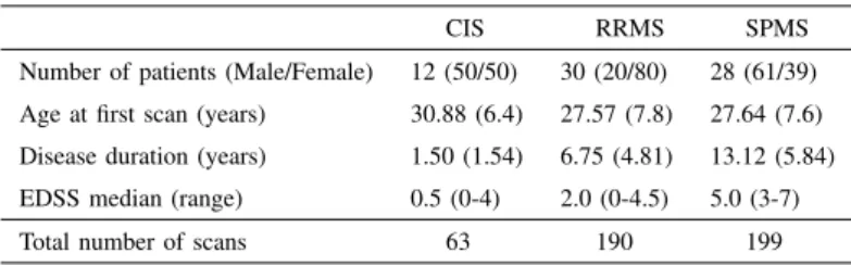
In this study, seventy MS patients distributed across three clinical forms (CIS, RRMS and SPMS), as shown in Table I, are considered. Each patient underwent multiple brain MRI examinations over a different period, ranging from 2.5 to 6 years. The minimum number of scans per patient is 3, while the maximum is 10. The gap between two consecutive scans is either 6 or 12 months. The total number of MRI scans in the dataset is 452.
For each patients, the structural brain connectivity was generated, by combining brain grey matter (GM) parcellation, obtained after segmentation of T1-weighted MR images, and the WM fiber-tracking, reconstructed from DTI acquisitions. More formally, as described in Kocevar et al. [18], after labelling each voxel of the T1-weighted MR images in four classes [WM, cortical GM, sub-cortical GM, cerebro-spinal fluid (CSF)], a segmentation of the cortical and sub-cortical GM was performed on the T1 images. Meanwhile, a prepro-cessing of DTI data was performed using the Eddy-current distortions correction [19], and a probabilistic streamline fiber-tracking algorithm was applied to generate WM fiber-bundles. The generation of these fiber-bundles used as connections between the GM nodes led to the construction of a symmetrical connectivity matrix A ∈ Nq×q+ where q = 84 for each patients.
Specifically, the adjacency matrix A is generated by summing the number of streamlines connecting each pair of nodes and represents a weighted undirected graph G = (V, E, ω), where |V | = q defines the set of brain regions, |E| = m represents the set of connections between these regions while ω defines the number of fibers connecting two nodes.
B. Notation
If not clearly stated, we will use the notation described in [20]. We denote with lower case letters e.g. a scalar values,
TABLE I
DEMOGRAPHIC INFORMATION OFMSPATIENTS OF DIFFERENT CLINICAL PROFILES(CIS, RR, SP).
CIS RRMS SPMS Number of patients (Male/Female) 12 (50/50) 30 (20/80) 28 (61/39) Age at first scan (years) 30.88 (6.4) 27.57 (7.8) 27.64 (7.6) Disease duration (years) 1.50 (1.54) 6.75 (4.81) 13.12 (5.84) EDSS median (range) 0.5 (0-4) 2.0 (0-4.5) 5.0 (3-7) Total number of scans 63 190 199
with bold lower case letters e.g. aaa 1-dimensional vectors, with uppercase letter e.g. A matrices and with Euler script letters A tensors. Matrices with superscripts e.g. X(n)define the factor matrices obtained from the factorisation while ˆX(n) defines
the unfolding of a tensor of mode n. Practically speaking, for a tensor of 3rd oder, ˆX(0)
∈ R(i×j∗z)+ denotes the mode 0,
ˆ
X(1) ∈ R(z×i∗j)
+ denotes the mode 1 and ˆX(2) ∈ R (j×i∗z) +
denotes the mode 2.
C. Random walk
Let’s consider an undirected weighted graph G = (V, E, ω) where |V | = n and |E| = m. A walk, of length p on the graph G is a sequence of connected vertices H[v0] = [v0, · · · , vr]
such that |H[v0]| = p and v0 is defined as starting
ver-tex. Following this notation, we can also define a walk as a sequences of weighted edges representing the connection between two consecutive nodes: W [v0] = [w0, · · · , ws] such
that |W [v0]| = |H[v0]| − 1 = s where wi is the weight of
the edge connecting the two nodes (vq, vz). In the rest of
this paper we refer to a walk according to its weighted edges representation.
A random walk can be modelled as k-th order Markov Chain, in which the future state depends only on the current state and is independent from the last k − 1 previous states. In general, a k-th order random walk is generated by sampling the position i-th, given the current state, from the transition probability distribution:
P r[wi|wi−1, wi−2, wi−s] = P r[wi|wi−1] (1)
Under the Markov Chain assumption, this probability is non-zero if there is an edge between vertex vi and vi−1.
Moreover, in order to generate a k-th order Markov Chain random walks, we need to sample the k initial vertices in order to effectively calculate the transition probability. Henceforth, the random process that defines the starting point of a first order random walk is characterised by a specific probability distribution that is usually independent from all the others paths that starts from a different position inside the graph. Given n random walks of length s a multiple Markov Chain sequences of edge weights is defined. By stacking all the sequences horizontally, it is possible to construct a matrix M ∈ R(n×s).
Fig. 1. Visual representation of the tensor describing a patient
D. Tensorization
Tensors are multidimensional arrays of numerical values and therefore generalise matrices to multiple dimensions. Using the tensor formalism, it is possible to obtain a compact 3-dimensional representation of longitudinal brain connectivity pathways. More in detail, in the proposed approach, each pa-tient is represented by a third-order tensor generated from the bi-dimensional representation of the random walks obtained for each time step. As an example, the tensor Xi∈ R(n×s×t)
can be defined for the patient i, where n is the number of random walks, s is the length (in terms of number of weighted edges) of the walk, and s is the number of scans available for the specific i-th patient. A visual representation of such a tensor is proposed in Figure 1.
A number of different factorization algorithms have been proposed in the literature, such as Higher Order SVD (HOSVD) [21], Tucker decomposition [22], Canonical polyadic decomposition (CPD) [23] and Non-negative Tensor Factorization (NTF) [24]. In this work, the NTF approach is used as all the values of the tensor are non-negative. Moreover, it is desirable for the decompositions to retain the non-negative characteristics of the original data and thereby facilitate the results interpretation.
E. Non-Negative tensor factorization (NTF)
Generally speaking, an n-order tensor has rank one if it can be written as the outer product of n nonzero vectors. The rank of a tensor is defined as the minimal number of rank-1 terms that generate the tensor as their sum. In this work we will use the NTF. More precisely, it defines an N -order tensor X ∈ Rd1×d2×···×dn as a sum of K rank-1 terms:
X =JX(1), X(2), ..., X(n) K = K X r=1 xxx(1)r(1)r(1)r ◦x (2) r x(2)r x(2)r ◦x(3) r x(3)r x(3)r ◦...◦x(n) r xx(n)r(n)r +E (2) where J.K defines the factorization operation, X defines the original N -order tensor, K defines the rank, and E ∈ Rd1×d2×···×dn is the residual tensor. The symbol “◦”
repre-sents the outer product.
Considering a third-order tensor as an example, equation (2) can be defined as a system of equations as defined in (3):
X XX ≈ x(3)1 xx(3)1(3)1 x(2)1 xx(2)1(2)1 x(1)1 xx(1)1(1)1 + . . . + xxx(3)R(3)R(3)R xxx(2)R(2)R(2)R xxx(1)R(1)R(1)R
Fig. 2. Canonical polyadic decomposition with rank R of a 3rd order tensor
ˆ X(1)= (X(1)◦ X(2))X(3)T ˆ X(2)= (X(1)◦ X(3))X(2)T ˆ X(3)= (X(2)◦ X(3))X(1)T (3) On the other hand, ˆX(1), ˆX(2), ˆX(3) define the unfolding of
the original tensor X of type 0, 1 and 2 respectively. Multiple types of algorithms has been proposed in order to minimize the loss:
L = ||X − ˆX || ≈ ||X −JX(1), X(2), X(3)
K||
2 F
In this work, the Alternating Least Square (ALS) algorithm is employed which implies the recursive optimisation of each of the component as defined in the following equation:
X(1) ← arg min X(1)∈R + || ˆX(1)− (X(1)◦ X(2))X(3)T|| X(2) ← arg min X(2)∈R + || ˆX(1)− (X(1)◦ X(3))X(2)T|| X(3) ← arg min X(3)∈R+ || ˆX(2)− (X(2)◦ X(3))X(1)T|| (4) F. Method description
Goal of this study is to exploit longitudinal information in order to detect latent temporal anomalies useful for distin-guishing between early and severe MS clinical phenotypes. Longitudinal variations and tissue damage evolutions are in-trinsically different between MS patients in the very early phase of the disease (CIS) and the RRMS course compared to the more severe stage of the illness as in the SPMS course.
For each patient, brain connectivity matrices are first gener-ated and the random walk matrices are computed according to Section II-C. Then, a multi-view tensor is obtained by stack-ing together multiple random walk matrices, as previously described in Section II-D. It is worth to note that each random walk can be interpreted as a feature describing the connections between different regions (nodes) of the brain network for a single patient in a specific time step. In order to make different features for different time steps comparable, a L1-norm is applied.
The third-order tensor is decomposed by means of NTF, thus producing a combination of 3 rank-k matrices as defined in equation (3). Specifically, matrix Xi(3) captures the longitu-dinal variation of patient i while matrices Xi(1) and Xi(2) represent the latent factors describing the random paths and their relative edges respectively. In this study, the rank k of
the NTF was fixed at 10 since higher values do not result in a meaningful improvement of the reconstruction error while increasing the computational cost. The number of random path was set to 100 and their length to 20, which provided the more stable results.
In order to detect the most anomalous edges in the multi-view tensor, Xi(1)and Xi(2)are combined. Let x(1)be a generic component of Xi(1) and let x(2) be a generic component of
Xi(2). Let dx(1) be the the percentile distribution of the values
in x(1) and let d(2)
x be the the percentile distribution of the
values in x(1). Thus, two sets of indices can be computed as
follows:
Sx(1)= {j | d(1)x j> 2σ(1), ∀j ∈ 1, . . . , |d(1)x |}
Sx(2) = {w | d(2)x w> 2σ(2), ∀w ∈ 1, . . . , |d(2)x |}
where σ(1) is the standard deviation of d(1)x and σ(2) is the
standard deviation of d(2)x . It is worth to note that each pair
(s1, s2) ∈ Sx(1) × Sx(2) identify a precise location inside
the multi-way tensor, thus refer to a precise edge inside a precise random path. The set of anomalous edges in the original tensor is obtained by repeating the procedure for each component in Xi(1) and Xi(2). Finally, the brain regions (i.e. nodes) connected by the anomalous edges are selected.
The described process is summarised in Algorithm 1. In order to increase the readability of the proposed method, a schematic visual representation of the entire process is depicted in Figure 3.
The proposed method can be thought of as a realisation of an event conditioned to a specific random sampled input. Although not exactly randomly defined, Markov Chain based random walks can convey some statistical properties that nicely couple with a completely randomly sampled approach [25]. In addition, they provide a meaningful embedding strat-egy compared to drawing edges at random [26].
It should be emphasised that the above described method is applied iteratively adopting a Monte Carlo strategy. The process is repeated 100 times, recording the anomalous edges at each iteration. The most occurring nodes are selected as outlier, indicating anomalous longitudinal changes in the brain. G. Unsupervised classification
The above described method produces, for each patient, a frequency distribution which summarises the likelihood of a specific node to be identified as anomalous. Notwithstanding, the primary goal of this work is to classify clinical profiles. In order to achieve such result k-means clustering was applied to the obtained distributions in order to retrieve a label assignment for each patient.
III. RESULTS
In this section, we report the details of our experimental work. First, a two-way comparison was performed between the three clinical forms herein considered (CIS, RRMS and SPMS). Second, we combined patients in the early and pri-mary phase of the disease (CIS+RRMS) together and compare
Fig. 3. Schematic representation of the proposed method applied recursively 100 times for each subject. Starting from DTI+T1 images, for each subject with multiple time acquisitions, a set of longitudinal adjacency matrices (A) is created. k-order random walks is then applied to each of these matrices and a new longitudinal random walk embedding is generated (B). Tensorization in thus performed on the embedding matrices in order to obtain an higher order tensor X . Factorial components X(1), X(2), X(3)are obtained by applying NTF. Finally, factor X(1)and X(2)are combined and a set of anomalous nodes can be
identified. Repeating the entire process 100 times for each subject, a vector of frequency distribution of anomalous nodes is created for each patient. Stacking horizontally all the subject’s anomalous nodes frequencies, a matrix of anomalies (C) is produced. By applying k-means on this matrix a label is assigned to each subject and the classification task can be performed.
them with patients in the secondary phase (SPMS). Third, a statistical analysis of the results was performed and some interesting insights are provided.
A. Classification
In Table II, we report the results obtained with our method. Four different measures are considered to evaluate the classi-fication task. In order to have a measure of reproducibility, the entire process was repeated 10 times with different initialisa-tion for both the k starting points of the k-order random walks and for the starting values of the factorization components.
In order to evaluate the classification results, the following metrics were considered: P recision = T P +F PT P , Recall =
T P
T P +F N, F 1 =
2∗precision∗recall
precision+recall and the Area Under the
Curve (AUC weighted score). The CIS vs SPMS group reported the best results with an F1 score of 76.67 (5.01) and AUC score of 76.33 (5.68). Notwithstanding, the highest variability for both measures is also observed probably due to the low dimensionality of the dataset and high level of unbalance between classes. On the other hand, the RRMS vs SPMS group highlighted the lowest score with an F1 and AUC score of 70.17 (3.37) and 70.00 (3.29) respectively. As far as the CIS+RRMS vs SPMS group is concerned, an F1 of 74.17 (3.66) and an AUC of 73.83 (3.60) is reported.
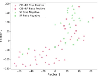
Afterwards, a graphical analysis is considered for all the comparisons discussed above. In order to better visualise the clustering results, t-distributed stochastic neighbour embed-ding (t-SNE) [27] dimensionality reduction technique was employed. It is worth to note that in the t-SNE procedures,
the perplexity parameter dictates the shape of the mapping function. For this reason, we performed multiple evaluations for different level of the parameter starting from a value of 5 to 30 at steps of 5. In Figure 4, the k-means clustering result ob-tained comparing CIS and SPMS groups is pictured. Although the data were highly imbalanced, a clear separation between patients groups is visible (CIS represented in red while SPMS represented in green). SPMS patients widely spread across space causing some degree of uncertainty in the clustering. Once again, this might be due to the high level of imbalance observed in the longitudinal data. In Figure 5, the RRMS vs SPMS comparison shows a good level of separation between groups though a minimum overlap is noticeable. Finally in Figure 6, we reported the comparison between the CIS+RRMS and SPMS patients’ groups. In agreement with what is shown in Figure 4 and Figure 5, a nice overall separation appears between early and advanced clinical courses.
B. Statistical Analysis
As allowed by our approach, we are interested in detecting the graph’s nodes, which provide latent temporal anomalies useful for distinguishing between primary and secondary MS clinical courses. In this purpose, a statistical analysis is performed in order to better understand and investigate the implication of the obtained results. In particular, we focus on the RRMS vs SPMS comparison.
For each brain region (node), we counted the number of times a node is considered anomalous by our method. Figure 7, depicts the average node-to-node difference of the anomaly
Algorithm 1: Proposed Method Data: P : set of patients;
Tp: number of acquisitions for the patient p;
q: number of vertices in G(V, E, ω); k: number of factors;
υ: total number of iterations;
Θp: anomaly count for each node of patient p;
Θ: anomaly frequencies for each patient; Φ: k-means label;
Input: Ap,t ∀p ∈ P ∀ t ∈ {0, 1, ..., Tp} longitudinal
matrices for each patient Output: Φ ∈ {0, 1}p label assignment Θ = [];
for p ∈ P do
Θp = {node0: 0, node1: 0, ..., nodeq : 0};
for iter ← 1 to υ do
1. Xp← create a tensor by performing n-order
random walks on Ap,t ∀t ∈ {0, 1, ..., Tp};
2. ˆX(1), ˆX(2), ˆX(3) ← N T F (X p);
for each factor do
3. Sx(1) ← select indices corresponding to
anomalous random walks
4. Sx(2) ← select indices corresponding to
anomalous edges for (i, j) ∈ Sx(1)× Sx(2) do Θp[nodei]+ = 1 Θp[nodej]+ = 1 end end end append(Θ, Θp) end Φ ← k-means(Θ); return: Φ; TABLE II
MEAN AND STANDARD DEVIATION(IN PARENTHESIS)OF CLASSIFICATION RESULTS
Group Comparison CIS vs SP RR vs SP CIS+RR vs SP F1 76.67 (5.01) 70.17 (3.37) 74.17 (3.66) Precision 79.33 (4.63) 77.67 (5.24) 77.50 (3.39) Recall 76.17 (4.31) 70.83 (2.99) 74.33 (3.33) AUC 76.33 (5.68) 70.00 (3.29) 73.83 (3.60) Note: RRMS and SPMS are reported as RR and SP respectively for better
visualisation purpose.
Fig. 4. CIS vs SPMS clustering visualisation using t-SNE dimensionality reduction
Fig. 5. RRMS vs SPMS clustering visualisation using t-SNE dimensionality reduction
count between RRMS and SPMS patients (red horizontal line defining the median anomaly frequency difference). More precisely, the height of the bins represent the mean node-to-node difference between the two clinical forms. Basically, for each Monte Carlo iteration, we first calculate the average node anomaly frequency for each patient (see section II-F) and average the result conditioned on the class label. Second, we take the node-to-node difference between clinical profiles. We repeat this process one hundred times and average the results. Conversely, in order to detect the brain structural differences between the average person in an early stage and compare it with the average person in the advance stage of the disease (SPMS), one hundred random walks of length 20
Fig. 6. CIS+RRMS vs SPMS clustering visualisation using t-SNE dimen-sionality reduction
Fig. 7. Node-to-node difference between RRMS vs SPMS: height of the bins represent the mean node-to-node difference between clinical profiles while colours define the node-to-node mean difference based on the occurrence of random walks
are performed for each patient and the node-to-node average difference between clinical profiles is considered. Specifically, for each patient, we first count the number of time a node is included in a k-order random walk. Second, the node-to-node average was considered as a condition of the class label. We then calculate the node-to-node difference of the average values between clinical profiles. We repeated this process one hundred times and average the results. For interpretability purposes, we rescale the values in the range [0, 1] and colour the bins based on this score. The obtained random-walk-based average difference can be considered as a score that defines the structural difference between an average patient in the primary phase of the disease (CIS and RRMS) and the average patient in a more advance stage (SPMS). However, it does
Fig. 8. Node-to-node difference score between RRMS vs SPMS for node with value greater than the median (red line Figure 7). Node colours represent the degree of anomaly score difference between clinical profiles
not take into account the longitudinal component resulting in a possible biased estimator for the real structural difference between clinical profiles.
Notwithstanding, in Figure 7 it is possible to notice that most of the brain areas with high value of anomaly frequency difference are also the area that register the greatest structural difference between the two clinical groups being compared. This suggest that our method mainly focus on the most structurally important differences, neglecting the areas less relevant and that do not constitute central hubs inside the brain network (dark coloured bins).
To better visualise the location of the anomalous nodes, Figure 8 depicts the brain location of the nodes with anomaly values greater than the median (red line in Figure 7). The brain areas detected by our method are: right and left superior-parietal, right and left inferior-parietal, right and left inferior-temporal, right and left superior-temporal, right and left middle-temporal, left superior-frontal, right rostralmiddle-frontal, left caudate between just the most relevant one. Interestingly, although not the primary aim of this work, the selected areas are most often correlated with the brain areas commonly damaged by MS [28].
IV. DISCUSSION
The results obtained by the proposed method show the capability of our algorithm to discriminate between different MS clinical forms. The results in terms of Precision, Recall, F1 and AUC suggest that the proposed method is promising in order to perform unsupervised analysis of brain network. Moreover, we enriched our analysis by showing different plot by applying t-SNE on the factorization results. From the obtained images, some interesting properties are visible. More in detail, in Figure 5, good level of separation is observed between groups though a minimum overlap is also noticeable. This is expected since different patients entered in the study at different phases of the disease. In particular, some RRMS patients entered in the study with a high lesion load although with a reasonably low value of both Expanded Disability Sta-tus Scale (EDSS) and Multiple Sclerosis Functional Composite (MSFC) score. Moreover, some SPMS patients entered in the study with a lesion load comparable with the worst RRMS
scenario although reporting a much greater disability scores. This marginal overlap between the clinical forms makes the classification task more challenging resulting in some degree of misclassification.
In Figure 6, a wide spread of RRMS and SPMS patients can be observed, in line with the comparison previously discussed. Indeed, it is reasonable to argue that although labeled as early and advanced stage MS patients, some RRMS and SPMS patients experience a widely worsen or milder condition with respect to other patients equally labeled.
V. CONCLUSION
In this work we described a tensor-based method analyse for longitudinal changes in brain network of MS patients. More in detail, we provided an algorithm capable to exploit the longi-tudinal variations in order to perform classification of different forms of multiple sclerosis. We formalised our problem using the TF framework by modelling the longitudinal evolution of the brain graphs as a tensor. We then validated our algorithm on a real dataset of MS patients showing its capability to well discriminate between different MS clinical forms. As future work we plan to better analyse the latent factors obtained by the factorization and, at the same time, improve the quality of the results by taking into account external cofounding factors. Moreover, NTF could be too restrictive for some applications as it does not model all variability in the data [29]. We plan to increase the performance using block term decomposition (BTD) instead of CPD. Indeed, using a BTD model, it is possible to model the variability on the data by performing a so-called rank (Lr, Lr, 1) BTD [29].
REFERENCES
[1] Dobson R., Giovannoni G., “Multiple sclerosis: a review,” European journal of neurology, vol. 26, no. 1, pp. 27–40, 2019.
[2] Lublin F. D., Reingold S. C, Cohen J. A, Cutter G. R, Sørensen, others, “Defining the clinical course of multiple sclerosis: the 2013 revisions,” Neurology, vol. 83, no. 3, pp. 278–286, 2014.
[3] Ciccarelli, O., Werring, D. J., Barker, G. J., Griffin, C. M., Wheeler-Kingshott, C. A., Miller, D. H., & Thompson, A. J., “A study of the mechanisms of normal-appearing white matter damage in multiple sclerosis using diffusion tensor imaging,” Journal of neurology, vol. 250(3), pp. 287–292, 2003.
[4] Stamile C., Kocevar G., Cotton F., Maes F., Sappey-Marinier D., Sabine V. H., “Multiparametric non-negative matrix factorization for longitudinal variations detection in white-matter fiber bundles,” IEEE journal of biomedical and health informatics, vol. 21, no. 5, pp. 1393– 1402, 2016.
[5] Stamile C., Kocevar G., Cotton F., Sappey-Marinier D., “A genetic algorithm-based model for longitudinal changes detection in white matter fiber-bundles of patient with multiple sclerosis,” Computers in biology and medicine, vol. 84, pp. 182–188, 2017.
[6] Kocevar, G., Stamile, C., Hannoun, S., Cotton, F., Vukusic, S., Durand-Dubief, F., Sappey-Marinier, D., “Graph theory-based brain connectiv-ity for automatic classification of multiple sclerosis clinical courses,” Frontiers in neuroscience, vol. 10, no. 478, 2016.
[7] Charalambous, T., Tur, C., Prados, F., Kanber, B., Chard, D. T., Ourselin, S., Toosy, A. T. , “Structural network disruption markers explain disability in multiple sclerosis,” J Neurol Neurosurg Psychiatry, pp. 90(2), 219–226, 2019.
[8] Kocevar, G., Stamile, C., Hannoun, S., Cotton, F., Vukusic, S., Durand-Dubief, F., Sappey-Marinier, D., “Graph theory-based brain connectivity for automatic classification of multiple sclerosis clinical courses,” Fron-tiers in neuroscience, pp. 10, 478, 2016.
[9] Bokai C., Chun-Ta L., Xiaokai W., Yu P.S., Alex D. L., “Semi-supervised tensor factorization for brain network analysis,” in Joint European Conference on Machine Learning and Knowledge Discovery in Databases. Springer, 2016, pp. 17–32.
[10] Cao B., He L., Wei X., Xing M., Yu P. S., Klumpp H., Leow A. D., “t-bne: Tensor-based brain network embedding,” International Conference on Data Mining, 2017.
[11] Liu Y., He, L., Cao B., Yu P. S., Ragin A., Leow A., “Multi-view multi-graph embedding for brain network clustering analysis,” Thirty-Second AAAI Conference on Artificial Intelligence, 2018.
[12] Mahyari A., Zoltowski D., Bernat E., Aviyente S., “A tensor decomposition-based approach for detecting dynamic network states from eeg,” IEEE Transactions on Biomedical Engineering, vol. 64, 2016. [13] Khambhati A.N., Medaglia J.D., Karuza E.A., Thompson-Schill S.L., Bassett D.S., “Subgraphs of functional brain networks identify dynami-cal constraints of cognitive control,” Computational Biology, vol. 14(8), 2018.
[14] Cao B., Lu C., Wei X., Yu P. S., Leow A. D., “Semi-supervised tensor factorization for brain network analysis,” Machine Learning and Knowledge Discovery in Databases, vol. 9851, 2016.
[15] Cai D., He X., Han J., Huang T. S., “Graph regularized nonnegative matrix factorization for data representation,” IEEE Transactions on Pattern Analysis and Machine Intelligence, vol. 8, pp. 1548–1560, 2011. [16] Guixiang M., Lifang H., Chun-Ta L., Weixiang S., “Multi-view clus-tering with graph embedding for connectome analysis,” Association for Computing Machinery, 2017.
[17] Stamile C., Kocevar, G., Cotton, F., Maes, F., Sappey-Marinier, D., Sabine V. H., “Multiparametric non-negative matrix factorization for longitudinal variations detection in white-matter fiber bundles,” IEEE journal of biomedical and health informatics, vol. 24, no. 4, pp. 1137– 1148, 2020.
[18] Kocevar G., Stamile C., Hannoun S., Cotton F., Vukusic S., Durand-Dubief F., Sappey-Marinier D., “Graph theory-based brain connectivity for automatic classification of multiple sclerosis clinical courses,” Fron-tiers in neuroscience, vol. vol 13, 2019.
[19] Smith SM., Jenkinson M., Woolrich MW., Beckmann CF. et al., “Ad-vances in functional and structural mr image analysis and implementa-tion as fsl,” FSL. Neuroimage, vol. vol 62, 2019.
[20] Brett W., Bader T., Kolda G., “Tensor decompositions and applications,” SIAM, vol. 51, 2009.
[21] Lathauwer L.D., Moor B. D., Vandewalle J., “A multilinear singular value decomposition,” SIAM J. Matrix Anal. Appl, vol. 21(4), pp. 1253– 1278, 2000.
[22] Tucker L. R., “Some mathematical notes on three-mode factor analysis,” Psychometrika, vol. 31, pp. 279–311, 1966.
[23] Harshman R.A., “Methods of three-way factor analysis and multidimen-sional scaling according to the principle of pro-portional profiles,” PhD thesis, University of California, Los Angeles, CA, 1976.
[24] Shashua A., Hazan T., “Non-negative tensor factorization with applica-tions to statistics and computer vision,” In ICML, pp. 792–799, 2005. [25] Jerrum M., “Mathematical foundations of the markov chain monte carlo
method,” Springer, vol. 16, 1998.
[26] Sajjad H. P., Docherty A., Tyshetskiy Y., “Efficient representa-tion learning using random walks for dynamic graphs,” ArXiv, vol. abs/1901.01346, 2019.
[27] Hinton G.E.. Van der Maaten L.J.P., “Visualizing high-dimensional data using t-SNE,” Journal of Machine Learning Research, vol. 2579-2605, 2008.
[28] Han X.M., Tian H.J., Han Z., Zhang C., Liu Y., Gu J.B., Bakshi R., Cao X., “Correlation between white matter damage and gray matter lesions in multiple sclerosis patients,” Neural Regeneration Research, vol. 12(5), pp. 787–794, 2017.
[29] Hunyadi B., Camps D., Sorber L., Van Paesschen W., Sabine V. H., De Lathauwer L., “Block term decomposition for modelling epileptic seizures,” EURASIP Journal on Advances in Signal Processing, 2014.