HAL Id: hal-00296164
https://hal.archives-ouvertes.fr/hal-00296164
Submitted on 27 Feb 2007
HAL is a multi-disciplinary open access
archive for the deposit and dissemination of
sci-entific research documents, whether they are
pub-lished or not. The documents may come from
teaching and research institutions in France or
abroad, or from public or private research centers.
L’archive ouverte pluridisciplinaire HAL, est
destinée au dépôt et à la diffusion de documents
scientifiques de niveau recherche, publiés ou non,
émanant des établissements d’enseignement et de
recherche français ou étrangers, des laboratoires
publics ou privés.
observations
J. Lelieveld, C. Brühl, P. Jöckel, B. Steil, P. J. Crutzen, H. Fischer, M. A.
Giorgetta, P. Hoor, M. G. Lawrence, R. Sausen, et al.
To cite this version:
J. Lelieveld, C. Brühl, P. Jöckel, B. Steil, P. J. Crutzen, et al.. Stratospheric dryness: model
simula-tions and satellite observasimula-tions. Atmospheric Chemistry and Physics, European Geosciences Union,
2007, 7 (5), pp.1313-1332. �hal-00296164�
www.atmos-chem-phys.net/7/1313/2007/ © Author(s) 2007. This work is licensed under a Creative Commons License.
Chemistry
and Physics
Stratospheric dryness: model simulations and satellite observations
J. Lelieveld1, C. Br ¨uhl1, P. J¨ockel1, B. Steil1, P. J. Crutzen1,2, H. Fischer1, M. A. Giorgetta3, P. Hoor1, M. G. Lawrence1, R. Sausen4, and H. Tost1
1Max Planck Institute for Chemistry, J. J. Becherweg 27, 55128 Mainz, Germany 2Scripps Institution of Oceanography, UCSD, La Jolla, CA 92093-0221, USA 3Max Planck Institute for Meteorology, Bundesstrasse 53, 20146 Hamburg, Germany 4DLR-Institut f¨ur Physik der Atmosph¨are, Oberpfaffenhofen, 82234 Wessling, Germany
Received: 20 October 2006 – Published in Atmos. Chem. Phys. Discuss.: 14 November 2006 Revised: 19 February 2007 – Accepted: 22 February 2007 – Published: 27 February 2007
Abstract. The mechanisms responsible for the extreme dry-ness of the stratosphere have been debated for decades. A key difficulty has been the lack of comprehensive models which are able to reproduce the observations. Here we examine re-sults from the coupled lower-middle atmosphere chemistry general circulation model ECHAM5/MESSy1 together with satellite observations. Our model results match observed temperatures in the tropical lower stratosphere and realisti-cally represent the seasonal and inter-annual variability of water vapor. The model reproduces the very low water va-por mixing ratios (below 2 ppmv) periodically observed at the tropical tropopause near 100 hPa, as well as the char-acteristic tape recorder signal up to about 10 hPa, providing evidence that the dehydration mechanism is well-captured. Our results confirm that the entry of tropospheric air into the tropical stratosphere is forced by large-scale wave dynamics, whereas radiative cooling regionally decelerates upwelling and can even cause downwelling. Thin cirrus forms in the cold air above cumulonimbus clouds, and the associated sed-imentation of ice particles between 100 and 200 hPa reduces water mass fluxes by nearly two orders of magnitude com-pared to air mass fluxes. Transport into the stratosphere is supported by regional net radiative heating, to a large extent in the outer tropics. During summer very deep monsoon con-vection over Southeast Asia, centered over Tibet, moistens the stratosphere.
1 Introduction
Even though the stratosphere is very dry compared to the troposphere, water is central in radiative and chemical pro-cesses, including ozone depletion. In the energy budget of the lower stratosphere the emission of thermal infrared (IR)
Correspondence to: J. Lelieveld
radiation, mostly by H2O and CO2, is a main cooling term
(Mlynczak et al., 1999). Further, H2O chemistry is the
pri-mary source of hydroxyl (OH) radicals, which initiate oxida-tion processes and destroy ozone (Solomon, 1999). Impor-tant oxidation reactions by OH include the release of ozone destroying halogen radicals from HCl and HBr, and the con-version of CH4 into CO2 and 2H2O. The latter reaction is
an important source of water in the middle and upper strato-sphere, whereas in the lower stratosphere transport from the troposphere is prevalent (Remsberg et al., 1996). Despite the stratospheric dryness, temperatures can be low enough for water to condense, for example, into polar stratospheric clouds. Heterogeneous reactions on these clouds and the sed-imentation of ice particles play a key role in the formation of the ozone hole.
More than half a century ago Brewer (1949) explained the dryness of the stratosphere by the large-scale ascent of air across the tropical tropopause, acting as a “cold trap”. Ow-ing to the negative temperature lapse rate in the troposphere, and the high and consequently very cold tropical tropopause, the air is “freeze-dried” at stratospheric entry. Although this general concept has been corroborated since (e.g. Holton et al., 1995), the locations and actual mechanisms controlling the freeze-drying have been subject of debate for decades, spawned by the discovery of a water vapor minimum (hy-gropause) a few kilometers above the tropopause (Kley et al., 1979).
The cold trap concept implies that cirrus clouds develop near the tropical tropopause, and the moisture is removed by the gravitational settling (sedimentation) of ice particles. If this were a general feature, cirrus would occur ubiqui-tously throughout the tropics, which is not observed. Since the 1980s several theories have evolved to account for spa-tially confined dehydration. On the one hand, deep convec-tive penetration (overshooting) and localized rapid updrafts were emphasized (Danielsen, 1982; Sherwood and Dessler, 2001). On the other hand, particular fountain regions were
identified at the tropical tropopause where temperatures are very low so that the cirrus clouds can form during slow ascent (Newell and Gould-Stewart, 1981; Jensen et al., 2001).
Additional explanations have been pursued to reconcile the presence of deep convection below the tropopause and stratospheric dehydration aloft, for example, by assuming convective excitement of gravity waves that propagate up-ward, cool the air in the wave crests and thus generate ice clouds (Potter and Holton, 1995), or by assuming a com-bination of dehydration mechanisms (V¨omel et al., 2002). Both the gradual upwelling and convective processes leave a distinct water vapor isotope ratio in the lower stratosphere, and measurements of hydrogen and oxygen isotopes in H2O
have shown that to some extent both processes are involved (Webster and Heymsfield, 2003).
Satellite measurements from the early 1990s onward have greatly improved the time-height view of water vapor in the lower tropical stratosphere (Russell et al., 1993). Mote et al. (1996) have used these measurements to demonstrate the seasonal dependence of the freeze-drying effect, with cold-est and dricold-est tropopause conditions during boreal winter (December-March). They showed that the dehydration sig-nal is carried deeper into the stratosphere up to about 10 hPa, and dubbed this phenomenon the tropical tape recorder. The upward motion of the water vapor minimum in the tape recorder also explains the location of the hygropause (Kley et al., 2000).
More recently, trajectory studies based on meteorological analyses have elucidated the transport pathways through the tropical tropopause region during which the air masses are dehydrated (Bannister et al., 2004; Bonazzola and Haynes, 2004; Fueglistaler et al., 2004, 2005). It was shown that the upper troposphere over the western Pacific Ocean is a major ascent region, and that the upper level monsoon circulation plays an important role in the transport deeper into the strato-sphere. Furthermore, stratospheric chemistry-climate mod-els have been developed to simulate dynamical, radiative and chemical processes. Despite recent advancements, there is a large spread in simulated water vapor fields, including the representation of the tape recorder and the location of the hy-gropause (Eyring et al., 2006).
Here we present results of a new atmospheric chem-istry general circulation model (AC-GCM) that describes the lower and middle atmosphere (Giorgetta et al., 2006; J¨ockel et al., 2006). The global scale of the model precludes that we explicitly compute convection and cloud microphysical de-tails. Nevertheless, we show that the model reproduces ob-served dynamical features and tracer distributions, including the tropical tape recorder.
In the next section we review some main aspects of strato-spheric radiation and dynamics to provide a context for our AC-GCM simulation results and to understand the desicca-tion mechanism. This secdesicca-tion may be skipped by readers who are familiar with the literature. Subsequently we present our model and the satellite data used, comparisons of the
differ-ent datasets and their interpretation, and we address the role of features that are not resolved by our AC-GCM. Finally we summarize the processes that control the dryness of the stratosphere.
2 Stratospheric dynamics and radiation
The stratospheric circulation is driven by the following main influences. Firstly, the differential solar heating of the strato-spheric ozone layer in the winter hemisphere, i.e. between high latitudes in polar night and sunlit latitudes, causes large meridional temperature differences and hence a poleward pressure gradient. The additional effect of the Coriolis force on the rotating Earth generates the westerly circumpolar flow in the extra-tropics, giving rise to the observed polar vortices. Secondly, extra-tropical wave disturbances, excited in the troposphere by land-sea contrasts, flow over mountains and synoptic weather systems, can propagate into the strato-sphere when the flow is westerly, and exert a drag force onto the circumpolar westerlies. This deceleration of the polar vortex alters the balance between the pressure gradi-ent and Coriolis effects, which induces a residual meridional circulation towards the winter pole and a sinking motion in high latitude winter (Haynes et al., 1991). Differences in the land-sea distribution and orography cause stronger winter-time wave effects on the stratospheric vortex in the Northern Hemisphere (NH) than in the Southern Hemisphere (SH).
The stratospheric mass balance is maintained by ascent near the equator, analogous to a fluid-dynamical suction pump drawing air upward and poleward from the tropical tropopause at about 100 hPa (∼16 km altitude) (Holton et al., 1995). In the tropical middle and upper stratosphere the up-welling is augmented by solar short-wave radiative heating (via O3)although this is partly balanced through IR cooling
by CO2and O3(Mlynczak et al., 1999). In the tropical lower
stratosphere IR cooling by H2O is counteracted by IR
heat-ing by O3, and on average net heating/cooling rates are small
(Gettelman et al., 2004a), generally less than 1 K/day. The IR radiative effects of O3and H2O have a pronounced spatial
distribution (Highwood and Hoskins, 1998; Norton, 2001), and our model results presented below show that regional dif-ferences substantially influence troposphere-to-stratosphere transport.
It is important to distinguish a transition region between the tropical troposphere and stratosphere between about 12 and 18 km altitude (i.e. about 200 and 75 hPa), called the tropical tropopause layer (TTL) (Highwood and Hoskins, 1998; Folkins et al., 1999). It has been proposed to de-fine the TTL more accurately in terms of net radiative heat-ing, but we argue against it because both the sign and the magnitude of this term vary strongly with the presence of cumulonimbus anvils and cirrus clouds. The latter can be found throughout the depth of the TTL (Wylie and Wang,
1997; Dessler et al., 2006) and have a substantial impact on the heating profile (Hartmann et al., 2001; Corti et al., 2006). By and large, upward motion below the TTL is governed by cumulonimbus convection, whereas above the TTL it is controlled by the large-scale dynamics. Thus both for the troposphere and the stratosphere the relevant process under-standing is relatively well established, whereas for the TTL the picture is more ambiguous. This partly results from the fact that vertical velocities in the TTL are small and difficult to measure, especially above extensive cumulonimbus anvils. Furthermore, it is clear that the initial impact of cumulonim-bus convection is moistening because these clouds carry sat-urated air and condensates into the upper troposphere and TTL (Soden, 2004; Luo and Rossow, 2004, Gettelman et al., 2006a). Therefore, an explanation of stratospheric dryness will need to reconcile the direct moistening and indirect de-hydration attributes of convection.
The coldest parts of the TTL are found over the areas with most extensive deep convection, notably over the western Pa-cific Ocean warm pool (Seidel et al. 2001). In these cold regions thin cirrus clouds can be formed, also known as sub-visual or subvisible cirrus (Wylie and Wang, 1997). These ice clouds can desiccate the air by ice particle sedimentation (Jensen et al., 2001), and our model results presented be-low show that this process is most efficient between 200 and 100 hPa.
Here we focus on the geographic region where upward motion predominates in the lower stratosphere, between 30◦N and 30◦S latitude (Rosenlof, 1995). We consider the ten year period 1996–2005 for which model calculations have been performed and satellite data are available. The pressure altitudes on which we concentrate our model eval-uation are ∼100 hPa, approximately representing the tradi-tional climatological tropopause in the middle of the TTL, and 70–75 hPa, near the top of the TTL where dehydrated air enters into the stratosphere.
3 Numerical model
The atmospheric chemistry GCM used in our study cou-ples the 5th generation European Centre – Hamburg model, ECHAM5 (version 5.3.01) (Roeckner et al., 2003, 2006) to the 1st Modular Earth Submodel System, MESSy1. This model - abbreviated E5M1 - includes a comprehensive rep-resentation of tropospheric and stratospheric cloud, radi-ation, multiphase chemistry and emission-deposition pro-cesses (J¨ockel et al., 2006). The model has a spectral dynam-ical core, computing the atmospheric dynamics up to wave number 42 using a triangular truncation (T42), while physi-cal and chemiphysi-cal parameterizations are physi-calculated on the as-sociated quadratic Gaussian grid at a resolution of about 2.8◦ in latitude and longitude (Roeckner et al., 2006).
The vertical grid used here resolves the lower and mid-dle atmosphere with 90 vertical layers from the surface to a
top layer centered at 0.01 hPa (∼80 km altitude). The mean layer thickness in the lower and middle stratosphere is about 700 m, sufficient to resolve vertically propagating waves with vertical wavelengths of 2.8 km and longer, which is a prereq-uisite to realistically simulate the quasi-biennial oscillation (QBO) (Giorgetta et al., 2006). In the tropopause region the vertical resolution is even higher, about 500 m (6–10 hPa).
Prognostic variables, predicted on the basis of fundamen-tal (primitive) equations in spectral space, i.e. temperature, divergence, vorticity, (the logarithm of) surface pressure, and those in grid point space such as specific humidity, cloud liq-uid and ice water and chemical tracers, are calculated every 15 min (at T42 resolution). Orographic and non-orographic gravity waves are parameterized in ECHAM5 (Manzini et al., 2006, and references therein). A similar setup of the non-orographic gravity wave parameterization was used in Manzini et al. (2003) and Steil et al. (2003). Details of the model setup are provided in J¨ockel et al. (2006); note that we use the S2 model setup described in that article.
ECHAM5 has been coupled with MESSy1, which com-prises a modular interface structure that connects submod-els to the dynamical core model (J¨ockel et al., 2005; see also www.messy-interface.org). The tracer advection is cal-culated with a mass conserving flux form semi-Lagrangian scheme (Lin and Rood, 1996). The ECHAM5 radiation scheme distinguishes four UV-VIS and near-IR, and 16 ther-mal IR spectral regions (Wild and Roeckner, 2006), and it utilizes the online computed tracer distributions. Photolysis rate calculations for the troposphere up to the mesosphere are based on the eight spectral band approach described in Land-graf and Crutzen (1998), considering absorption and scat-tering by gases, aerosols and clouds in a delta-two-stream method.
Detailed chemistry calculations are performed using a ki-netic preprocessor (Sandu and Sander, 2006), applying a Rosenbrock solver, to describe a set of 177 gas phase, 57 photo-dissociation and 81 heterogeneous tropospheric and stratospheric reactions (Sander et al., 2005). Details of the chemical mechanism (including reaction rate coefficients and references) can be found in the electronic supplement of J¨ockel et al. (2006) (http://www.atmos-chem-phys-discuss. net/6/1/2006/acpd-6-1-2006-supplement.zip).
For the representation of natural and anthropogenic emis-sions and dry deposition of trace species, including microm-eteorological and atmosphere-biosphere interactions, wet de-position by large-scale and convective clouds, multiphase chemistry and polar stratospheric clouds, we refer to the de-tailed descriptions by Ganzeveld et al. (2006), Kerkweg et al. (2006a,b) and Tost et al. (2006a,b). The results of the tropospheric and stratospheric chemistry calculations, using a number of diagnostic model routines, have been tested against in situ and satellite measurements (J¨ockel et al., 2006).
Cloud convection is described using the method presented in Tiedke (1989), which assumes that an ensemble of clouds
modifies the large-scale environmental dry static energy and specific humidity. The scheme distinguishes three types of convection (Roeckner et al., 2003): i) Penetrative, deep con-vection, triggered by moisture convergence exceeding evapo-ration, in which entrainment is proportional to the large-scale moisture convergence; ii) Shallow convection, mostly trig-gered by subcloud layer turbulence; and iii) Midlevel con-vection originating at higher altitudes, e.g. frontal clouds in extra-tropical cyclones, where the cloud base and entrain-ment are determined by the large-scale flow.
An addition to the convection routine by Nordeng (1994) accounts for organized entrainment/detrainment in deep con-vection, and mass closure based on convective available po-tential energy. An intercomparison of different convection schemes in ECHAM5 has shown that the present model setup produces a realistic hydrological cycle, including clouds, precipitation and water vapor distribution in the upper tropo-sphere and lower stratotropo-sphere (Tost et al., 2006b). The con-vective tracer transport calculations use a monotonic, posi-tive definite and mass conserving algorithm following a bulk approach (Lawrence and Rasch, 2005; Tost, 2006).
The model scheme for stratiform clouds includes prognos-tic equations for liquid and ice water and for the higher or-der moments of total cloud water (Roeckner et al., 2003). The description of cloud physics includes rain formation by coalescence, the aggregation of ice crystals into snowflakes, accretion of cloud droplets by falling snow, gravitational settling of hydrometeors and phase transition processes (Lohmann and Roeckner, 1996). Between 238 K and 273 K a mixed cloud phase is assumed, whereas at lower tempera-tures the condensed water is only in the form of ice.
The parameterizations of cloud processes are relatively de-tailed for a GCM, and include condensation/evaporation of liquid water, deposition/sublimation of ice, evaporation of rain, sublimation of snow, autoconversion of cloud droplets, accretion of cloud droplets by precipitation, homogeneous, stochastical-heterogeneous and contact freezing of droplets, and aggregation of ice crystals and melting of cloud ice (Lohmann and Roeckner, 1996). Nevertheless, the cloud pa-rameterizations only account for cloud bulk properties, not for microphysical details such as droplet and crystal number concentrations. A description of the ECHAM5 simulated hy-drological cycle is presented in Hagemann et al. (2006).
The growth of ice crystals below temperatures of 238 K takes place by the deposition of water vapor. At temperatures above 238 K water vapor deposition only takes place if cloud ice is already present. The size distribution of ice crystals is based on an empirical relationship between the effective par-ticle radius of the ice crystal distribution and the ice water content derived from aircraft observations. The sedimenta-tion of ice particles is also parameterized through an empiri-cal description, representing observed ice mass precipitation rates (Heymsfield and Donner, 1990). The model calculated mean ice water content of cirrus clouds over the equatorial Pacific Ocean compare well with ice measurements in the
205–270 K temperature interval (Lohmann et al., 1995; Mc-Farquhar and Heymsfield, 1996).
In order to analyze the transport fluxes of air and water in its different phases, we apply the ATTILA Lagrangian transport scheme (Reithmeier and Sausen, 2002), for which the model atmosphere is subdivided into about 1 700 000 air parcels of constant mass (ATTILA: Atmospheric Tracer Transport In a Lagrangian model). The scheme applies a fourth order Runge-Kutta method for advection, and we em-ploy it diagnostically as an on-line forward trajectory model. The results of this method have been tested against a trajec-tory model using data of the European Centre for Medium-range Weather Forecasts (ECMWF) (Stohl and Trickl, 1999; Traub, 2004).
The online coupling of the ATTILA transport scheme into our AC-GCM prevents time interpolation errors typical for trajectory models, and it is fully mass conserving. Each of the computed forward trajectories has a “clock” to determine the moment at which a certain boundary is surpassed. The selected boundaries are the 200, 100 and 75 hPa pressure lev-els in our AC-GCM. Since two-way transport can occur over such boundaries, we apply a residence time criterion of 96 h to define an exchange event as “almost irreversible” (Wernli and Bourqui, 2002). In addition, we performed these calcu-lations across isentropic surfaces, i.e. the potential tempera-ture levels 340, 380 and 420 K, roughly compatible with the above pressure levels.
4 Model nudging
GCMs can be applied to simulate atmospheric conditions over extended periods, and the results of such simulations can be statistically compared with climatologies based on long-term observations or to other model simulations. For at-mospheric chemistry and stratospheric water vapor computa-tions this is more difficult because extended data sets are rare, and it is more challenging to apply statistical techniques in model evaluation. Therefore, we follow the strategy of nudg-ing the model toward realistic meteorological conditions, so that an evaluation of model results against observations is less dependent on the size of the datasets and a direct com-parison becomes more meaningful.
In addition to prescribed sea surface temperatures, the model has been nudged towards realistic meteorological con-ditions for the period 1996–2005, based on ECMWF op-erational analyses, by adding a Newtonian relaxation term to the four above mentioned prognostic variables in spec-tral space, i.e. vorticity, divergence, temperature and surface pressure (Van Aalst et al., 2004). Several precautions pre-vent the excitement of spurious waves. Firstly, the ECMWF data are projected onto the model levels and surface orogra-phy by a interpolation procedure developed by I. Kirchner, Free University of Berlin (personal communication), based on the method described in Majewski (1985). Secondly, the
Zonal wind at 2°N - 2°S in m/s (positive is west) MJS DM JS D M JS DM JS D M JS DM JS D M JS DM JS D M JS DM JS D 1996 1997 1998 1999 2000 2001 2002 2003 2004 2005 70 60 50 40 30 20 10 0 -10 -20 -30 -40 -50 -60 -70 -80 0.01 0.1 1.0 10.0 100.0 Pre ssu re (h Pa )
Fig. 1a. Model calculated equatorial wind, showing the SAO in the
mesosphere and upper stratosphere and the QBO in the middle and lower stratosphere.
nudging strengths are very low (about 10−5s−1), with a 6 h relaxation e-folding time for vorticity, 24 h for temperature and surface pressure and 48 h for divergence. Thirdly, a slow-normal-mode filter is applied to the nudging data, which re-moves the fast components (Daley, 1991).
Finally, we avoid inconsistencies between the ECHAM5 and the ECMWF boundary layer representations by leaving the lowest three model levels free (apart from surface pres-sure), while the nudging increases stepwise in four levels up to about 706 hPa. The nudging tapers off to zero at 204 hPa to allow unconstrained simulations of the TTL and stratosphere. From the perspective of the present study, the T42/2.8◦and 90 layer resolution of the model is sufficiently high for the TTL and upward, though relatively low for the troposphere. The latter limitation is made up for by nudging the tropo-spheric part of the model using ECMWF data, which have been computed at much higher resolution.
We emphasize that it is important not to nudge the pa-rameters and processes that directly control water vapor and chemical tracers, and only optimize boundary conditions for the model-data comparison. Since the nudging is weak, the model reproduces the actual meteorology approximately but not exactly, so we still need to rely on some statistical com-parison with measurement data. Below we will compare probability density functions from model output and satellite measurements of stratospheric water vapor.
Figure 1 presents the results of the 10-year E5M1 simu-lation used in the present study, showing that the model re-alistically simulates the Semi-Annual Oscillation (SAO), the QBO and the stratospheric tape recorder. A comparison with measured tropical wind reversals in the QBO is presented by J¨ockel et al. (2006) for a coupled atmospheric-GCM simu-lation, by Giorgetta et al. (2006) for a model version with-out chemistry, and additional evaluation against satellite ob-servations is presented below. These simulation results are available on request (http://airdata.mpch-mainz.mpg.de).
Zonal mean water vapor at 10°N - 10°S in ppmv
MJS DM JS D M JS DM JS D M JS DM JS D M JS DM JS D M JS DM JS D 1996 1997 1998 1999 2000 2001 2002 2003 2004 2005 0.01 0.1 1.0 10.0 100.0 Pre ssu re (h Pa ) 7.0 6.5 6.0 5.5 5.0 4.5 4.0 3.5 3.0 2.5 2.0 1.5 1.0 0.5
Fig. 1b. Water vapor in the tropical middle atmosphere and the
characteristic tape recorder signal, discernable for about 1.5 years after entrance into the stratosphere at about 100 hPa.
5 Satellite data
A long time series of stratospheric water vapor measure-ments is available from the Halogen Occultation Experi-ment (HALOE) on the Upper Atmospheric Research Satel-lite (UARS) (Russell et al., 1993). The instrument operated from the fall of 1991 until November 2005, thus providing an extensive data set to compare with our model simulations for the 1996–2005 time period. The comparison between model and satellite data focuses on 1997–2005, thus omitting 1996, because the first year is too close to the initial conditions of the model, which were based on HALOE data over the five years prior to the simulation period.
HALOE was a solar occultation limb sounder operating in the near-IR during sunrise and sunset; water vapor was measured in the 6.6 µm channel. An advantage of solar oc-cultation instruments is that a relative measurement is per-formed, i.e. the ratio between solar radiation outside the atmosphere and that minus atmospheric attenuation. This technique may be conceived as self-calibrating and suffers little from instrument drifts, which is particularly useful for long-term observations. HALOE provided global coverage in the stratosphere and mesosphere at a vertical resolution of about 2 km, with a total accuracy within about ±10% over much of the height range and decreasing to ±30% near the tropopause (Harries et al., 1996). A disadvantage of HALOE was that the number of measured profiles was rel-atively small, and global coverage was only achieved within about a month. Secondly, we use data from the Michelson Interferometer for Passive Atmospheric Sounding (MIPAS) on the European Environmental Satellite (ENVISAT). MI-PAS is a high-resolution Fourier transform spectrometer, a limb scanning sounder operating in the near- and mid-IR, i.e. 4.15–14.6 µm (Fischer and Oelhaf, 1996). The instrument has been operational since the summer of 2002, and provides global coverage with 14–15 orbits per day at a horizontal resolution of 300–500 km and a vertical resolution of about 3 km. Here we use MIPAS temperature data for the period
Al ti tu d e (h Pa ) 7.0 6.5 6.0 5.5 5.0 4.5 4.0 3.5 3.0 2.5 2.0 1.5 1.0 Zonal mean water vapor (ppmv) at 5°N - 5°S
MJSDMJSDMJSDMJSDMJSDMJSDMJSDMJSDMJSDMJS 1996 1997 1998 1999 2000 2001 2002 2003 2004 2005 E5M1 1 10 100 HALOE 1 10 100
Fig. 2. Zonal mean water vapor from HALOE satellite
measure-ments and E5M1 model calculations. The tick marks at the up-per bar indicate the points in time of the measurements. Note that HALOE measurements in the tropics are largely limited between about 5◦N and 5◦S latitude.
December 2002–November 2003. The potential bias of tem-perature measurements in the 10–35 km height interval has been assessed to be smaller than 0.5 K (Wang et al., 2005), with a total accuracy of individual data points (given as the square root of the quadratic sum of random and systematic errors) of 0.5–1.5 K. Finally, we use data from the Atmo-spheric Infrared Sounder (AIRS) on the NASA Aqua satellite (Aumann et al., 2006). This is a nadir scanning grating-array spectrometer, which measures in the 3.7–15.4 µm spectral region in >2000 spectral channels at a horizontal resolution of 50 km and a vertical resolution of 1–2 km from the surface up to the lower stratosphere. The instrument is operational since summer 2002. A comparison of AIRS temperature data with balloon sounding and in situ aircraft measurements in the upper troposphere and lower stratosphere indicates a to-tal accuracy within ±1.5 K near the tropopause (Gettelman et al., 2004b; Divakarla et al., 2006).
6 Results and discussion 6.1 Middle and upper stratosphere
Figure 1 shows the model calculated zonal wind in the equa-torial stratosphere (top) and zonal mean water vapor con-centrations between 10◦N and 10◦S latitude (bottom). The computed water vapor mixing ratios compare favorably with HALOE measurements, although the modeled amplitude of the seasonal cycle seems somewhat stronger (Fig. 2), as dis-cussed in more detail in subsequent sections. Since the
dif-ference between the model and HALOE data is similar to the total accuracy of the satellite measurements and data re-trieval, it seems reasonable to qualify this as good agreement. In earlier work it has been discussed that the signal of the QBO can be identified in tracer distributions, including ozone and water vapor (Randel et al., 1996; Giorgetta and Bengtsson, 1999; Geller et al., 2002). The QBO modulates the upward velocity of air in the tropical stratosphere, and the temperature signal can modify the specific humidity. Thefore, the accurate simulation of the QBO is required to re-alistically compute the tape recorder signal in water vapor (Giorgetta et al., 2006). Nevertheless, by comparing Figs. 1a and b the role of the QBO in the water vapor distribution is not clearly evident.
Closer inspection reveals that during the easterly phase at about 10 hPa the dry tongues reach to somewhat higher al-titudes than during the westerly phase. In an earlier model version the upward penetration of moist air seemed deeper during the easterly phase (Giorgetta and Bengtsson, 1999). However, in this earlier work the oxidation of methane was not considered, and it appears that during the westerly phase methane derived moisture has an increasingly stronger down-ward influence than in the easterly phase, which counteracts the QBO modulation of water vapor from below.
Interestingly, a rather strong influence is manifest from the SAO, where the westerly phase coincides with the most hu-mid conditions. From our model results we identify rela-tively narrow water vapor troughs in January and July and somewhat wider peaks in April and October in the upper stratosphere, possibly a few weeks earlier than seen in satel-lite data during the period 1992–1995 (Jackson et al., 1998). The troughs are strongest in boreal winter, and they seem to progress downward with a few hPa/month. This effect may include a meridional advection component that gives rise to anomalies that wax and wane in winter and summer, respec-tively. It is also interesting to note in Fig. 1a that the west-erly phase of the QBO starts after the westwest-erly phase of the SAO has progressively reached lower altitudes in the strato-sphere, suggestive of a causal relationship between the SAO and QBO.
In the upper stratosphere there is a clear relationship be-tween dryness and the easterly phase of the SAO, during which tropical dehydrated air is transported upward more ef-ficiently. The relatively large interannual variability in the easterly phase coincides with relatively large variability in water vapor, whereby the lowest water vapor mixing ratios occur during the strongest easterlies, which relates to the strength of the planetary wave forcing. Conversely, during the downward propagation of the westerly phase below the westerly jet upward transport of dry air is reduced.
6.2 Lower stratosphere
Although the long time-span of the HALOE data series is unique, for the lower tropical stratosphere the comparison
6.0 5.5 5.0 4.5 4.0 3.5 3.0 2.5 2.0 1.5 1.0 20°N 0° 20°S 0° 100°E 160°W 60°W DJF MAM JJA SON 20°N 0° 20°S 20°N 0° 20°S 20°N 0° 20°S
Water vapor mixing ratio at 100 hPa, Dec 2002 - Nov 2003 (ppmv)
2 3 3 3 3 3 3 3 3 3 3 4 3 4 5 4 4 3 4 4 4 4 3 3 4 4
Fig. 3. Model calculated water vapor (ppmv) during four seasons at the model level nearest to 100 hPa (97 hPa) for the period December
2002 to November 2003.
between modeled and measured water vapor is hampered by the sparseness of satellite observations, especially near 100 hPa. The HALOE water vapor retrieval is affected by thin cirrus cloud “contamination”, and since these clouds oc-cur in very cold regions of active dehydration, as discussed in the next section, it is conceivable that the data are biased. Furthermore, by interpolating sparse HALOE data to display long-term tendencies, as shown in Fig. 2, the variability and seasonal cycle of water vapor, being particularly strong near 100 hPa, are suppressed. The limited number of profiles from which Fig. 2 (top panel) is constructed is indicated at the up-per bar, whereby many of these profiles do not reach down to 100 hPa.
To circumvent these problems, we performed a direct point-to-point comparison between both data sets by sam-pling the model results (from 5 hourly output) as closely as possible to the location and time periods of the HALOE mea-surements. We reiterate that we cannot expect that the ap-plied nudging procedure leads to an exact mimicking of the synoptic variability, and we must also accept sampling er-rors related to the different resolutions of the data sets. Note the vertical resolution of HALOE is coarser than the model, and the averaging kernel of the HALOE data retrieval is not available to replicate the data sampling from the model. Nev-ertheless, it may be expected that such errors are relatively minor and appear as random noise in the statistical analysis.
MIPAS-E5M1 comparison Dec 2002 - Nov 2003 70 hPa, 30°N-30°S (No. of events 7643) R=0.94 model satellite 0.5 0.4 0.3 0.2 0.1 0.0 Pro b a b ili ty 0.4 0.3 0.2 0.1 0.0 180 190 200210220230240 Temperature (K) model T e mp e ra tu re (K) sa te lli te 240 230 220 210 200 190 180 180 190 200210220230240 Temperature (K)
Fig. 4. Comparison of E5M1 temperature calculations with MIPAS
at 70 hPa for the period December 2002 to November 2003. The left panel shows a correlation plot, the red line representing ideal agree-ment, and R is the correlation coefficient. The right panels show the probability density distributions of the E5M1 model results and the MIPAS data.
In Fig. 3 we show model calculated water vapor mixing ratios at ∼100 hPa for four seasons during the period De-cember 2002 to November 2003. These images are quali-tatively consistent with previous analyses, e.g. of HALOE data by Randel et al. (2001), although these authors studied an earlier time period. The lowest water vapor mixing ratios
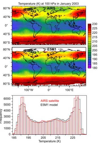
230 225 220 215 210 205 200 195 190 185 180 AIRS E5M1 100°W 0° 100°E Temperature (K) at 100 hPa in January 2003 80°N 40°N 0° 40°S 80°S 80°N 40°N 0° 40°S 80°S 185 195 205 215 225 Temperature (K) F re q u e n cy 6000 5000 4000 3000 2000 1000 0 E5M1 model AIRS satellite
Fig. 5a. Comparison of E5M1 temperature calculations with AIRS
satellite measurements at 100 hPa for January 2003. The upper panel shows the “ascending node” AIRS data, taken during day-light conditions outside the Arctic region, and the middle panel the corresponding daytime E5M1 results.
are found over the equatorial western Pacific Ocean during boreal winter (DJF). Highest water vapor mixing ratios, on the other hand, are found further north during boreal summer (JJA) over southern Asia, Central America and in particular over the western Pacific Ocean near 20◦N.
In the lower tropical stratosphere the low temperatures are a consequence of adiabatic cooling in the wave driven large-scale ascent, modulated by radiative heating or cooling, be-ing sensitive to spatial distributions of clouds, water vapor and ozone. Figure 4 shows that the model calculated tem-peratures at 70 hPa agree excellently with the MIPAS mea-surements during the same period in 2002–2003. The left panel in Fig. 4 shows a correlation plot (correlation coeffi-cient R=0.94). In the right panels we present the probability density functions (PDFs) of the model results and MIPAS data.
A comparison of the global model results with AIRS tem-perature data at 100 hPa is shown in Fig. 5, which corrob-orates the good agreement. The double-peaked frequency
distribution in Fig. 5a for January 2003 manifests the con-trasting temperatures between high and low latitudes and the transition zones at 200–220 K. Figure 5b presents the temperature distributions in July 2003, with a single peak around 195 K, reflecting the low temperatures in the tropics and partly also at high latitudes in the SH. A second peak, as seen in Fig. 5a, is missing because the relatively high-est temperatures are largely rhigh-estricted to high latitudes in the NH. The linear regression between the satellite observations and the model results, based on about 105 collocated data points per month, is 0.99, and the correlation coefficients are R=0.98 and 0.97 for January and July 2003, respectively.
We emphasize that MIPAS temperature data have a small mean bias of less than 0.5 K, and both MIPAS and AIRS temperature measurements have a total accuracy within
±1.5 K. For individual measurements, as compared in Figs. 4 and 5, the accuracy may be less, although especially the near-spectral AIRS measurements should be rather accurate. Based on the high correlations between model results and measurements, the realistically simulated spatial distribu-tions and PDFs we conclude that the model accurately re-produces temperatures in the tropical tropopause region and lower stratosphere. This is unlikely to be coincidental, and we interpret it as confirmation that the model realistically simulates the key dynamic and radiation processes.
The water vapor minima and maxima in Fig. 3 coincide with regions of lowest and highest temperatures, respectively (Seidel et al., 2001). It is known that water vapor and tem-perature correlate near the tropical tropopause, in line with the cold trap concept (Randel et al., 2004; Fueglistaler and Haynes, 2005). In Fig. 6 we investigate this correlation for the inner tropics (10◦S–10◦N) in our model results, based on
zonal mean temperature and water vapor. The correlation co-efficient is generally high year around for the pressure levels 200–90 hPa, R≥0.8, and it is highest in boreal winter when dehydration in the equatorial zone is particularly effective.
From April to September the correlation coefficient is lower, especially at 80 and 75 hPa, and it breaks down to R≤0.4 at 75 hPa during June–August. This is the time of year during which the TTL is strongly influenced by water vapor intrusions from the Asian monsoon (discussed in Sects. (6.4– 6.5). Particularly in the upper TTL the correlation between water vapor and temperature at 10◦S–10◦N during boreal summer diminishes because the transport processes that con-trol water vapor are to a large degree located in the outer tropics. Future work could further exploit the simultaneous water vapor and temperature measurements from satellites (e.g. MIPAS, AIRS) to study the spatial distribution of these parameters and regional differences within the tropics.
In Figs. 7 and 8 we compare the model results with HALOE water vapor data for the period 1997–2005 at the pressure levels 100 and 75 hPa, respectively. Both figures indicate that especially the lowest water vapor mixing ra-tios are simulated accurately, indicating that our model re-produces the dehydration mechanism. Both the model and
230 225 220 215 210 205 200 195 190 185 180 100°W 0° 100°E Temperature (K) at 100 hPa in July 2003 80°N 40°N 0° 40°S 80°S 80°N 40°N 0° 40°S 80°S 190 200 210 220 230 Temperature (K) F re q u e n cy 8000 6000 4000 2000 0 E5M1 model AIRS satellite AIRS E5M1
Fig. 5b. Comparison of E5M1 temperature calculations with AIRS
satellite measurements at 100 hPa for July 2003. The upper panel shows the “ascending node” AIRS data, taken during daylight con-ditions outside the Antarctic region, and the middle panel the corre-sponding daytime E5M1 results.
satellite data show that occasionally very low mixing ratios can occur at ∼100 hPa, down to nearly 1 ppmv. The correla-tion coefficients between both data sets for the three latitude bands shown are quite high, 0.63≤ R≤ 0.75.
Again, the right panels show the PDFs, providing sup-port for the good agreement at the low end of the water vapor distributions. Note that the tracer PDFs are sensitive to dynamics and mixing processes, and that non-Gaussian (e.g. long-tailed) distributions characterize irregular trans-port events (Sparling, 2000). The relatively large widths of the distributions indicate substantial variability, which seems to be underestimated in the model results. Especially to-ward the high end, above 3.5 ppmv, the modeled variability is underestimated compared to HALOE. Although the satellite data uncertainty is about ±30% for the lower stratosphere, the systematic nature of the model-measurement difference suggests that our model results may be biased, as discussed in more detail in Sect. 6.4.
The lower left panel of Fig. 7 indicates that in a few cases
75 hPa 80 hPa 90 hPa 100 hPa 200 hPa 1.0 0.8 0.6 0.4 0.2 J F M A M J J A S O N D Month C o rre la ti o n co e ff ici e n t
Zonal mean H2O - T correlation, 10°N - 10°S
Fig. 6. Model calculated correlation coefficients (R) between zonal
mean water vapor and temperature in the latitude band 10◦S to 10◦N at different altitudes for the period 1996–2005.
relatively high mixing ratios are calculated in locations that are dryer in the observations, which could be related to sam-pling errors or time shifts between computed and real events of high humidity at ∼100 hPa. Both in the model results and satellite data, the PDFs are wider at 10◦N–30◦N than
at 10◦S–30◦S. The PDF for the inner tropics at 10◦S–10◦N,
shown in the upper panel, is intermediate between both hemi-spheres. In Sect. 6.4 we compare modeled time series with HALOE data, and show that deviations between calculations and measurements are largest in the NH, associated with the Asian monsoon, and that the bias is time dependent, associ-ated with a drying tendency.
The model-measurement correlation plots and PDFs for 70 hPa in Fig. 8 are compacter and narrower than for 100 hPa, respectively. The agreement is again rather good, and the correlation coefficients are similar to those for 100 hPa, 0.60≤R≤0.77. The very low water vapor mixing ratios seen at 100 hPa are rare at 70 hPa, and data points below 2 ppmv are absent. The variability is generally less at 70 hPa as a re-sult of zonal and meridional mixing in the upper TTL. Both the correlation plots and the PDFs show best agreement to-ward low mixing ratios, and also reveal a lack of modeled variability in the upper part of the range. In the inner tropics at 10◦S–10◦N, shown in the upper panel of Fig. 8, the satel-lite measurements suggest a bimodal PDF, a consequence of moist events originating in higher latitudes. The model PDF only shows a weak bimodality as the peak at ∼3.5 ppmv is underrepresented.
6.3 Dehydration mechanism
Our model results show that water vapor mixing ratios at the tropical tropopause are not zonally uniform (Fig. 3), although
R=0.63 1 2 3 4 5 6 7 8 9 9 8 7 6 5 4 3 2 1 H2O (ppmv) model H2 O (p p mv) sa te lli te 0.3 0.2 0.1 0.0 1 2 3 4 5 6 7 8 9 H2O (ppmv) Pro b a b ili ty satellite model 0.2 0.1 0.0
100 hPa, 30°S-10°S (No. of events 4759) R=0.73 1 2 3 4 5 6 7 8 9 9 8 7 6 5 4 3 2 1 H2O (ppmv) model H2 O (p p mv) sa te lli te 0.3 0.2 0.1 0.0 1 2 3 4 5 6 7 8 9 H2O (ppmv) Pro b a b ili ty satellite model 0.2 0.1 0.0
100 hPa, 10°N-30°N (No. of events 4152) R=0.75 1 2 3 4 5 6 7 8 9 9 8 7 6 5 4 3 2 1 H2O (ppmv) model H2 O (p p mv) sa te lli te 0.3 0.2 0.1 0.0 1 2 3 4 5 6 7 8 9 H2O (ppmv) Pro b a b ili ty satellite model 0.2 0.1 0.0 HALOE-E5M1 comparison 1997-2005 100 hPa, 10°S-10°N (No. of events 1980)
Fig. 7. Comparison of E5M1 water vapor calculations with HALOE
at 100 hPa for the period 1997–2005.
the differences vanish upward through transport and mixing. Holton and Gettelman (2001) emphasized the relatively short time scale of horizontal relative to vertical transport in the TTL and stratosphere. The lower stratosphere is generally driest in the Indo-Pacific region during NH winter. The mod-eled temporal and vertical distribution of “dryness” in Fig. 9a clearly shows the lowest mixing ratios during the December-March period.
Figure 9 includes the accompanying temperature distribu-tion, illustrating that the driest regions (<2.5 ppmv) are also the coldest (<192 K). Furthermore, Fig. 9a demonstrates that occasionally the water vapor minimum is more distinct at 75 hPa, well above the tropopause, consistent with the ob-served hygropause. Although the hygropause is caused by the upward migration of the water vapor minimum in the tape recorder, it can be deepened by continuing dehydration above
R=0.61 1 2 3 4 5 6 7 8 9 9 8 7 6 5 4 3 2 1 H2O (ppmv) model H2 O (p p mv) sa te lli te 0.3 0.2 0.1 0.0 1 2 3 4 5 6 7 8 9 H2O (ppmv) Pro b a b ili ty satellite model 0.2 0.1 0.0
70 hPa, 30°S-10°S (No. of events 5423) R=0.77 1 2 3 4 5 6 7 8 9 9 8 7 6 5 4 3 2 1 H2O (ppmv) model H2 O (p p mv) sa te lli te 0.3 0.2 0.1 0.0 1 2 3 4 5 6 7 8 9 H2O (ppmv) Pro b a b ili ty satellite model 0.2 0.1 0.0
70 hPa, 10°N-30°N (No. of events 4977) R=0.60 1 2 3 4 5 6 7 8 9 9 8 7 6 5 4 3 2 1 H2O (ppmv) model H2 O (p p mv) sa te lli te 0.3 0.2 0.1 0.0 1 2 3 4 5 6 7 8 9 H2O (ppmv) Pro b a b ili ty satellite model 0.2 0.1 0.0
Figure 8
HALOE-E5M1 comparison 1997-2005 70 hPa, 10°S-10°N (No. of events 3710)Fig. 8. Comparison of E5M1 water vapor calculations with HALOE
at 70 hPa for the period 1997–2005.
the tropopause. Figure 9a also reveals that during NH win-ter the wawin-ter minima ascend from 100 to 75 hPa in about a month, i.e. at a mean speed of a few m/hour.
The tropical upwelling is brought about by the large-scale wave forcing, which has a maximum during December– March. Through adiabatic expansion and consequent cooling it contributes to the low tropopause temperatures (Yulaeva et al., 1994). The adiabatic cooling tends to be balanced by radiative heating (Holton et al., 1995), while on a regional scale heating may actually contribute significantly to the up-welling (Plumb and Eluszkiewicz, 1999). In the region be-neath the deep tropical convection produces anvil clouds, and above these clouds the heating is blocked and the upwelling decelerates. The deep convective clouds initially moisten the upper troposphere through the transport of saturated air, and the air is subsequently desiccated as it slowly travels through
30°N 15°N 0° 15°S 30°S
Zonal mean water vapor mixing ratio in ppmv
75 hPa 6.0 5.0 4.0 3.0 2.0 1.0 M J S D M JS DM JS D M JS DM JS DM JS DM JS DM JS D M JS D M JS D 1996 1997 1998 1999 2000 2001 2002 2003 2004 2005 30°N 15°N 0° 15°S 30°S 100 hPa
Fig. 9a. Time series of model calculated zonal mean water vapor
(ppmv) between 30◦N and 30◦S latitude, at the pressure altitude levels of about 100 and 75 hPa.
Zonal mean temperature in K
206 202 198 194 190 186 30°N 15°N 0° 15°S 30°S M J S D M JS DM JS DM JS DM JS DM JS DM JS DM JS DM JS DM JS D 1996 1997 1998 1999 2000 2001 2002 2003 2004 2005 30°N 15°N 0° 15°S 30°S 100 hPa 75 hPa
Fig. 9b. Time series of model calculated zonal mean temperature
(K) between 30◦N and 30◦S latitude, at the pressure altitude levels of about 100 and 75 hPa.
the TTL, also shown by observational and Lagrangian mod-eling studies (V¨omel et al., 2002; Jensen and Pfister, 2004).
Hence, the ascent through the TTL is accompanied by net cooling, which maintains a high relative humidity and sus-tains water condensation on upward advected particles. Our model results indicate that on average net radiative cooling up to several K/day is prevalent at ∼200 hPa throughout the year, while it decreases with altitude within the TTL. If the radiative cooling would be stronger it could balance the wave driven ascent and even contribute to subsidence (Fueglistaler and Fu, 2006). Figure 10 presents model calculated net ra-diative heating rates at the tropopause and in the lower strato-sphere for winter and summer 2003. These indicate that near the tropical tropopause at ∼100 hPa radiative heating prevails and therefore the cooling conditions are largely restricted to the layer beneath.
With increasing altitude in the TTL the O3
concentra-tion and the consequent radiative heating increase. However, thick convective clouds below can block the IR heating from
Radiative heating rates in 2003 in K/day
0.8 0.7 0.6 0.5 0.4 0.3 0.2 0.1 0 -0.1 -0.2 -0.3 January, 75 hPa January, 100 hPa July, 75 hPa July, 100 hPa 0° 100°E 160°W 60°W 20°N 0° 20°S 20°N 0° 20°S 20°N 0° 20°S 20°N 0° 20°S
Fig. 10. Model calculated net radiative heating rates at about 75 and
100 hPa in January and July 2003.
the lower troposphere so that freezing conditions are main-tained. As a result of continual saturation over ice within the coldest regions of the TTL, thin cirrus clouds are formed above the convective anvils. The presence of tropopause cirrus clouds has been confirmed by aircraft measurements (McFarquhar et al., 2000; Thomas et al., 2002; Peter et al., 2003), although it cannot be determined with confidence to what degree they are remnants of anvils or are formed within the TTL. In our model both are possible because water is transported in all phases. However, the modeled upward wa-ter transport is dominated by vapor, indicating that thin cirrus cloud presence is governed by in situ formation.
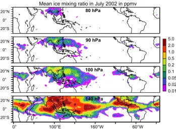
Figure 11 presents the model calculated mean ice water mixing ratios within the TTL. It shows TTL cirrus clouds, representing a mean water mixing ratio of a few ppmv at 150 hPa and about 0.1 ppmv at 100 hPa, which are largely collocated with deep convection, in agreement with satellite measurements (Wylie and Wang, 1997; Massie et al., 2002; Dessler et al., 2006). As long as the cirrus clouds overlie their cold cumulonimbus parents they contribute to radiative cooling. However, after the cumulonimbus anvils decay, the thin ice clouds become subjected to IR from the lower and warmer troposphere; hence, radiative heating intensifies and accelerates the transport into the stratosphere. Such radia-tively driven ascent of thin ice clouds is known as “cirrus lofting” (Corti et al., 2006).
Mean ice mixing ratio in January 2002 in ppmv 0° 100°E 160°W 60°W 5.0 2.0 1.0 0.5 0.2 0.1 0.05 0.02 0.01 80 hPa 90 hPa 100 hPa 140 hPa 20°N 0° 20°S 20°N 0° 20°S 20°N 0° 20°S 20°N 0° 20°S
Fig. 11a. Model calculated mean ice water mixing ratios (ppmv) at
about 140, 100, 90 and 80 hPa in January 2002.
Thus, the TTL drying results from the sedimentation of ice crystals that have formed within the TTL, mostly between 200 and 100 hPa altitude. Our model does not account for cirrus microphysical details and neglects the occurrence of supersaturation. This suggests that cloud formation, notably the amount of condensate, may not be very sensitive to these details, also indicated by sensitivity studies of Bonazzola and Haynes (2004). Nevertheless, observations show supersatu-ration is ubiquitous (Gettelman et al., 2006b), which indi-cates that the availability of ice nuclei may be a limiting fac-tor, i.e. delaying cloud formation. It is therefore conceivable that the number of ice nuclei affects the crystal size distribu-tion and consequently particle sedimentadistribu-tion rates and radia-tive properties, which should be studied in greater detail with advanced parameterization schemes.
In our model the drying is strongest between 200 hPa and the tropical tropopause, although some ice clouds extend to higher altitudes so that dehydration can continue aloft. A detailed comparison of Figs. 9 and 11 shows that the wa-ter minima can occur north of the cloud maxima, which is also observed from satellites (Randel et al., 2001), being the result of the northerly flow component in the regions of de-hydration. The ice clouds are actually sustained by horizon-tal transport of water vapor (Holton and Gettelman, 2001). Our model computes TTL cirrus clouds throughout the year; however, their location varies with that of deep convection and the cold regions aloft.
6.4 Moistening and drying periods
Figure 9 shows that during NH summer, both water vapor mixing ratios and temperatures in the tropical lower strato-sphere are substantially higher than in winter. Nevertheless, also in this season the coldest tropopause temperatures co-incide with the driest conditions. The winter and summer drying mechanisms are the same, i.e. cirrus cloud formation
Mean ice mixing ratio in July 2002 in ppmv
0° 100°E 160°W 60°W 5.0 2.0 1.0 0.5 0.2 0.1 0.05 0.02 0.01 80 hPa 90 hPa 100 hPa 140 hPa 20°N 0° 20°S 20°N 0° 20°S 20°N 0° 20°S 20°N 0° 20°S
Fig. 11b. Model calculated mean ice water mixing ratios (ppmv) at
about 140, 100, 90 and 80 hPa in July 2002.
and ice particle sedimentation above convective anvils, but the geographical locations and effectiveness differ.
The extra-tropical wave forcing in NH summer is about half that in winter, so that tropical upwelling and adiabatic cooling are reduced. The H2O contours at 100 hPa in Fig. 9a
appear at 75 hPa in about 2–3 months, i.e. traveling upward very slowly by about 1 m/hour. Our model generates the TTL cirrus further north than in winter (Fig. 11). Part of the TTL cirrus occurs over Southeast Asia, coincident with the very deep monsoon convection. Our model generates the deepest convection in this region, e.g. deeper than in the equatorial region during NH winter. Figure 11b shows that over South-east Asia the TTL cirrus can extend to relatively high alti-tudes. Consequently, the ice particles are more likely to evap-orate within the TTL rather than sediment large distances and contribute to dehydration.
Figure 9a shows that near the tropical tropopause (∼100 hPa) the meridional H2O distribution is relatively
dis-perse, i.e. affected by synoptic events, while the contours become more distinct with increasing altitude (75 hPa). This feature is related to meridional transport and mixing in the lower stratosphere (Rosenlof, 1995; Volk et al., 1996). Dur-ing NH summer the meridional transports extend relatively far north, controlled by the Tibetan High, a large quasi-stationary anticyclone in the upper troposphere and lower stratosphere, extending from the Mediterranean to the Pacific between about 10◦and 40◦N latitude.
It is located over the Asian monsoon surface trough and carries air poleward at its western flank over the Middle East and equatorward at its eastern flank near the Asian Pacific Rim. This air is relatively humid owing to the deep pen-etration of monsoon convection, and it plays a key role in moistening the stratosphere (Bannister et al., 2004; Gettel-man et al., 2004a; Fueglistaler et al., 2005; Fu et al., 2006). In Sect. (6.5) we address the associated transport routes and vertical fluxes of water vapor in more detail.
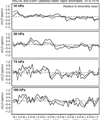
HALOE and E5M1 (dashed) water vapor anomalies, 10°S-10°N
Relative to long-term mean 10 hPa ∆ H2 O (p p mv) 1.2 0.8 0.4 0.0 -0.4 -0.8 -1.2 M J S D M J S D M J S D M J S D M J S D M J S D M J S D M J S D M J S 1997 1998 1999 2000 2001 2002 2003 2004 2005 50 hPa ∆ H2 O (p p mv) 1.2 0.8 0.4 0.0 -0.4 -0.8 -1.2 ∆ H2 O (p p mv) 1.2 0.8 0.4 0.0 -0.4 -0.8 -1.2 ∆ H2 O (p p mv) 1.2 0.8 0.4 0.0 -0.4 -0.8 -1.2 75 hPa 100 hPa
Fig. 12a. Tropical water vapor tendencies derived from HALOE
measurements (solid lines) and model calculations (dashed lines). Shown are the 2-monthly mean anomalies relative to the long-term mean.
During El Ni˜no events tropical tropopause temperatures can be increased, e.g. over the western Pacific region, and our model results for the strong El Ni˜no of 1997/98 show relatively high coincident water vapor mixing ratios, most pronounced at the end of the event in the summer of 1998. Nevertheless, in view of the inter-annual water vapor vari-ability near the tropical tropopause (Figs. 1 and 2) and at 75 hPa (Fig. 9a), it is not obvious that this El Ni˜no year was exceptional, especially during boreal winter. Both model and satellite data indicate similarly moist periods in the equato-rial lower stratosphere during non-El Ni˜no years, although our model seems to underestimate humidity at 100 hPa dur-ing the autumn and winter of 1997/1998.
Bonazzola and Haynes (2004) argued that during El Ni˜no and La Ni˜na years, both the regions of minimum temper-atures and transport pathways are shifted. Therefore, El Ni˜no events alter the regions of dehydration; however, they do not strongly influence the overall moisture transport into the stratosphere. In fact, our model results show that much of the inter-annual variability in water vapor, including in the 10◦N–10◦S latitude band, coincides with water vapor anomalies in the outer tropics, especially in the NH, sugges-tive of a link with the Asian monsoon.
In Fig. 12 we present long-term (red) and deseasonalized (black) tropical water vapor anomalies, derived both from
Relative to bimonthly mean
10 hPa ∆ H2 O (p p mv) 1.2 0.8 0.4 0.0 -0.4 -0.8 -1.2 M J S D M J S D M J S D M J S D M J S D M J S D M J S D M J S D M J S 1997 1998 1999 2000 2001 2002 2003 2004 2005 50 hPa ∆ H2 O (p p mv) 1.2 0.8 0.4 0.0 -0.4 -0.8 -1.2 ∆ H2 O (p p mv) 1.2 0.8 0.4 0.0 -0.4 -0.8 -1.2 ∆ H2 O (p p mv) 1.2 0.8 0.4 0.0 -0.4 -0.8 -1.2 75 hPa 100 hPa
HALOE and E5M1 (dashed) water vapor anomalies, 10°S-10°N
Fig. 12b. Tropical water vapor tendencies derived from HALOE
measurements (solid lines) and model calculations (dashed lines). Shown are the 2-monthly deseasonalized anomalies.
HALOE measurements and model calculations. Note this involves near point-to-point comparisons of these datasets as the model results were sampled at the locations closest to those of the HALOE measurements. We skip the first year (1996) because the model is too close to the initial condi-tions, as prescribed from HALOE data. We average over 2-monthly periods because the HALOE dataset is sparse, es-pecially at 100 hPa and since 2001. Figure 12 shows that the timing and amplitude of the seasonal and inter-annual variability in the model is remarkably similar to the HALOE observations, and Fig. 12a illustrates that the seasonal am-plitude falls off with altitude, hence the tape recorder signal vanishes.
From the HALOE water vapor measurements in the lower tropical stratosphere it appears that pre-2001 years were moister than the subsequent period (Fig. 2). Randel et al. (2006) analyzed HALOE data between 60◦S and 60◦N,
and concluded that stratospheric water vapor shows a sub-stantial and persistent decrease since 2001, linked to changes in the tropical tropopause and the large-scale circulation. Some caution with strong conclusions is called for, because the number of HALOE observations dropped by about a factor of two since 2001, and the sampling changed non-symmetrically between both hemispheres and between sun-rise and sunset occultation.
Notwithstanding these reservations, our analysis of tropi-cal water vapor from HALOE measurements (10◦S–10◦N)
in Fig. 12b confirms the occurrence of a negative anomaly at 100 hPa after the year 2000, being compelling because it seems to propagate upward in the tape recorder. This event is smaller in our model results and therefore we cannot provide a convincing explanation. Based on our model results we would rather classify it as variability. It should be stressed that the comparison presented here involves the exact pres-sure levels from the model, whereas the HALOE data repre-sent layers of a few kilometers thickness. If the satellite data would be available together with the averaging kernel of the retrieval algorithm, we could further improve the comparison and infer possible artifacts from vertical integration.
Interestingly, the drying event in 2001 may also be con-ceived as an episode that coincides with the solar cycle max-imum in 2000–2002, an issue that deserves further investi-gation. It may also be worth looking into a link with the Antarctic vortex split in SH spring 2002 since the water va-por anomaly arrived at about 10 hPa in September of that year, possibly associated with perturbed wave propagation. Alternatively, the episode may be interpreted as part of inter-decadal water vapor variability, given the very similar mixing ratios at the beginning and the end of the studied period, es-pecially at 100 and 75 hPa (Fig. 12).
A longer term negative tendency seems most apparent in the middle stratosphere at 10 hPa, both in the HALOE data and the model results (Fig. 12). In fact, by using all data from our model, i.e. not only the HALOE collocated subset in Fig. 12, we find a significant negative tendency of about 0.5 ppmv/decade in most of the stratosphere except in the extra-tropical lower stratosphere in the SH. Again, this points to the Asian monsoon, which will need to be investigated in greater detail.
In the upper stratosphere and mesosphere we must further-more account for a drying tendency since about 1997, asso-ciated with the solar cycle. In our model enhanced deple-tion of water vapor by Lyman-α photodissociadeple-tion continues until solar maximum in 2000–2002 (Fig. 1b). After 2002 this tendency reversed, to continue until solar minimum in 2007, which counteracts the overall negative tendency, al-though this is unlikely to have a strong influence on the trop-ical stratosphere. Further analyses of stratospheric water va-por trends should consider these multiple influences and the substantial inter-annual and inter-decadal variability, and in-clude longer term measurements and model calculations than the period considered here.
6.5 Troposphere-to-stratosphere fluxes
To determine vertical mass exchanges in the tropopause region we diagnostically applied the ATTILA Lagrangian transport scheme for the years 2002 and 2003. As indicated earlier, upward transport into the stratosphere is not restricted to the tropics, and the “turnaround” zones where the mean
vertical fluxes are just about zero are located at 30◦–35◦
(Rosenlof, 1995). We calculate that between 30◦N and 30◦S
the mean upward air mass flux across 200 hPa is 35.2×10⁹ kg/s, and the same amount of air descends poleward of 35◦ latitude. Approximately one quarter of the upward flux at 200 hPa subsequently enters the stratosphere at 100 hPa, in good agreement with an earlier estimate (Rosenlof and Holton, 1993), and ∼15% (5.8×10⁹kg/s) traverses 75 hPa.
Hence the TTL is to a large extent ventilated back into the troposphere, consistent with tracer measurements by aircraft suggesting a recirculation between the lower stratosphere and upper troposphere (Tuck et al., 1997). The accompa-nying annual upward water flux across 200 hPa is 7.8×10⁶ kg/s, while merely about 0.1% of this water mass, 11.2×10³ kg/s, reaches 75 hPa. This illustrates the high efficiency by which the air is desiccated, reducing the annual zonal mean water mixing ratio from roughly 100 ppmv at 200 hPa to 3– 3.5 ppmv at 75 hPa, whereby the desiccation largely occurs in the 100–200 hPa region.
Although CH4 oxidation strongly affects water vapor in
the upper stratosphere, it contributes relatively little to the overall stratospheric water loading. On average, approxi-mately 1.25×10³ kg/s CH4 is oxidized within the
strato-sphere, which produces less than 3×10³ kg/s H2O. Since
the annual mean upward H2O flux across the 100 hPa level
is about 23×103 kg/s, it follows that transport from the tropopause contributes more than 85%. By considering the H2O flux across 75 hPa this would be about 75%.
Furthermore, the above mentioned model calculated wa-ter mixing ratio at the stratospheric entry between 30◦N and 30◦S (3–3.5 ppmv) demonstrates that the annual mean
tropopause mixing ratio in the inner tropics, i.e. within 10◦
latitude from the equator (2–2.5 ppmv), is not representative of the overall moisture transport into the stratosphere, and that additional water is entrained from higher latitudes.
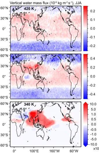
Figure 13 presents the model diagnosed vertical water mass fluxes across the isentropic levels of 340, 380 and 420 K, roughly equivalent to the 200, 100 and 75 hPa pres-sure levels. Here we use potential temperature rather than pressure coordinates to visualize areas of upward and down-ward motion, assuming that in absence of diabatic processes air parcels move along rather than across isentropic surfaces. Nevertheless, the annual mass fluxes across the isentropic and isobaric levels are similar (within ∼10%) but seasonally the differences can be larger. Comparing the lower panels of Fig. 3 to Fig. 11 illustrates that the upward moisture trans-ports in regions of strong convection coincide with the pres-ence of TTL cirrus. At 340 K upward motion is dominated by convection, while the picture entirely changes at 380 K (middle panels of Fig. 13).
In NH winter at the tropical tropopause the regions of strong convection and associated water transport over In-donesia and the western Pacific Ocean are characterized by relatively minor vertical motion at 380 and 420 K (Fig. 13a). Thus the geographic regions of strongest convective mass
60°N 30°N 0° 30°S 60°S 0° 100°E 160°W 60°W
Vertical water mass flux (10-9 kg m-2 s-1), DJF
0.4 0.2 0.0 -0.2 -0.4 60°N 30°N 0° 30°S 60°S 60°N 30°N 0° 30°S 60°S 0.2 0.1 0.0 -0.1 -0.2 420 K 380 K 340 K 5.0 10.0 1.0 0.5 -0.5 -1.0 -5.0 -10.0 x10³ 0.0
Fig. 13a. Model calculated water mass fluxes across the 340, 380
and 420 K isentropic surfaces, averaged for the periods December– February 2002 and 2003 in units 10−9kg m−2s−1(red is upward). Note the scale changes between panels.
fluxes in the troposphere are not the regions where air pri-marily enters the stratosphere. Based on operational wind data over Indonesia it has been shown that air mass fluxes at the tropopause can even be downward, thus represent-ing a stratospheric “drain” (Sherwood, 2000). Our model occasionally calculates descent over Indonesia at 100 hPa (380 K), although vertical velocities are very low. This regional inhibition of upward mass transport at the tropi-cal tropopause is caused by radiative cooling above the cold cloud tops, which rivals the extra-tropical wave driven up-welling. A relatively pronounced drain in our model occurs over the tropical Indian Ocean during NH summer (Fig. 13b). This phenomenon coincides with net radiative cooling at the tropopause over the extensive cumulonimbus anvils during a period when the wave-driving is weak, as shown in the lower panel of Fig. 10. As a consequence, the zonal av-erage vertical motion at 100 hPa during NH summer in the tropics is small or partly even downward, which can lead to shallow recirculation of air around the tropopause. At the
60°N 30°N 0° 30°S 60°S 0° 100°E 160°W 60°W 0.4 0.2 0.0 -0.2 -0.4 60°N 30°N 0° 30°S 60°S 60°N 30°N 0° 30°S 60°S 0.2 0.1 0.0 -0.1 -0.2 420 K
Vertical water mass flux (10-9 kg m-2 s-1), JJA
380 K 340 K 5.0 10.0 1.0 0.5 -0.5 -1.0 -5.0 -10.0 x10³ 0.0
Fig. 13b. Model calculated water mass fluxes across the 340, 380 and 420 K isentropic surfaces, averaged for the periods June– August 2002 and 2003 in units 10−9kg m−2s−1(red is upward). Note the scale changes between panels.
tropopause and in the lower stratosphere upward transport is stronger adjacent to the regions of strong convection and cumulonimbus anvil presence. Here H2O, O3and remnants
of TTL cirrus in the moist convective outflow contribute to net radiative heating, i.e. being subject to IR radiation from the lower troposphere, not blocked by the anvil clouds un-derneath. Therefore, at altitudes around 100–75 hPa (380– 420 K) upward motion and transport of water vapor to a large extent occurs between about 10◦and 30◦latitude (Fig. 13). This vertical transport pattern is most pronounced in South-east Asia, centered over the Tibetan Plateau (Fig. 13b), where convection is very deep, in agreement with the satellite data analysis by Fu et al. (2006).
Fu et al. (2006) hypothesized that convection by elevated surface heating over the Tibetan Plateau is particularly deep and detrains more water than elsewhere. Our model results support this hypothesis and corroborate that the ice particles formed in the deepest convective outflow are less likely to es-cape the TTL. The particles would have to grow to relatively