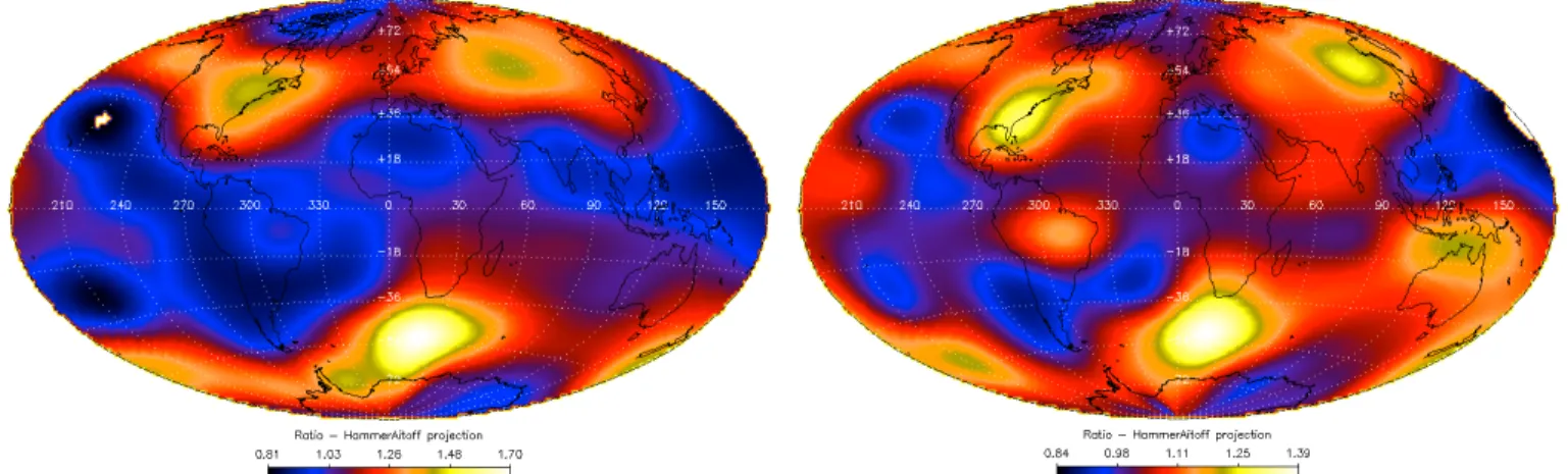
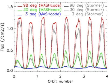
Improvements of FLUKA Calculation of the Neutron Albedo

HAL Id: cea-01851362

https://hal-cea.archives-ouvertes.fr/cea-01851362

Submitted on 30 Jul 2018

HAL is a multi-disciplinary open access

archive for the deposit and dissemination of

sci-entific research documents, whether they are

pub-lished or not. The documents may come from

teaching and research institutions in France or

abroad, or from public or private research centers.

L’archive ouverte pluridisciplinaire HAL, est

destinée au dépôt et à la diffusion de documents

scientifiques de niveau recherche, publiés ou non,

émanant des établissements d’enseignement et de

recherche français ou étrangers, des laboratoires

publics ou privés.

Boscher, Alfredo Ferrari, Markus Brugger

To cite this version:

Natacha Combier, Arnaud Claret, Philippe Laurent, Vincent Maget, Daniel Boscher, et al..

Im-provements of FLUKA Calculation of the Neutron Albedo. IEEE Transactions on Nuclear Science,

Institute of Electrical and Electronics Engineers, 2017, 64, pp.614 - 621. �10.1109/TNS.2016.2611019�.

�cea-01851362�

Abstract—This paper presents Monte-Carlo simulations based

on the Fluka code aiming to calculate the contribution of the neutron albedo at a given date and altitude above the Earth chosen by the user. Results consist of a two-parameter distribution, the neutron energy and the angle to the tangent plane of the sphere containing the orbit of interest, and are provided by geographical position above the Earth at the chosen altitude. In this paper, a major improvement was introduced with respect to the previous model concerning the filtering of incoming cosmic rays hitting the upper atmosphere. This more accurate estimation of neutron albedo is of prime importance for the radiation belts modelers because it constitutes the main source of protons > 40 MeV of the inner radiation belt.

Index Terms— Albedo, cosmic rays, CRAND, FLUKA, magnetosphere, neutrons

I. INTRODUCTION

HE performance level of imaging detectors operating at

Low Earth Orbit (LEO) is degraded due to the neutron albedo produced in the Earth atmosphere hit by incoming galactic cosmic rays (GCR). Generally, the background levels of space experiments strongly increase due to high particle flux encountered in the South Atlantic Anomaly (SAA) or near the polar regions during solar events, these particles being able to leave a trace on the detectors or activate their surrounding materials. However, the background level is so high during solar events or even when crossing the SAA, that imaging experiments are often switched off. Therefore, it is not uncommon that the albedo neutrons are the most important contribution to the background noise during normal operations outside the SAA. Most common background removal technics consist of estimating it by adjusting its level thanks to a function with two parameters, the geomagnetic latitude or the rigidity cutoff, plus a constant representing the internal background. The purpose of our model is to calculate the albedo neutron flux all around the Earth in order to disentangle better the two noise components (neutron albedo

N. Combier, A. Claret, and P. Laurent are with CEA-Saclay, DSM/IRFU/SAP, F-91191 Gif-sur-Yvette, France (e-mail: Natacha.Combier@cea.fr; Arnaud.Claret@cea.fr; Philippe.Laurent@cea.fr).

V. Maget, and D. Boscher are with Onera, The French Aerospace Lab, F-31055 Toulouse, France (e-mail: Vincent.Maget@onecert.fr; Daniel.Boscher@onecert.fr).

A. Ferrari, and M. Brugger are with CERN, CH-1211 Genève, Switzerland (email: Alfredo.Ferrari@cern.ch; Markus.Brugger@cern.ch).

and internal background). The neutron production in the atmosphere depends on various factors such as the flux of incoming galactic cosmic rays (GCR) reaching the Earth's neighborhood (anti-correlated with the solar cycle) and the Earth’s magnetic field (acting as an attenuating filter). In our model, the solar influence is taken into account by considering only the modulation of the GCR over the solar cycle, but not the protons emitted directly by the Sun and also reaching the Earth atmosphere. Most of the time, the latter contribution is negligible with respect to the first one, except during intense solar events. Once created in the atmosphere (mainly at 20 km altitude), part of these neutrons goes into space (the so-called albedo neutrons) where they undergo a beta decay (n ® p+ ₊ e– _{+ 𝜈}

e) due to their natural instability outside a nucleus. This process, called cosmic ray albedo neutron decay (CRAND), contributes to populate the inner Van Allen belt, which raises here another interest for calculating the albedo neutron flux all around the Earth.

The purpose of this paper is to present major improvements with respect to our former model [1]. The first improvement is relative to the geomagnetic filtering of incoming GCR, leading to a predicted flux of neutron albedo probably more representative of what is actually encountered at LEO altitude. The second improvement is relative to the spatial resolution of the predicted flux all around the Earth, which is more realistic in order to predict the encountered flux for a given orbit. The improvements of our model with respect to the previous one, in particular the geomagnetic filtering of incoming GCR, are described in Section II. The main characteristics of the obtained neutron flux are presented in Section III, and compared with previous results of the former model. Finally, results are discussed in Section IV and applications are presented in Section V.

II. MODEL

In this section, we remind readers of the main characteristics of the model already described in [1]. In particular, we detail in Section II.B the changes concerning the filtering of incoming particles and their transport with respect to the previous model.

A. Input particles

Incoming particles at the origin of the Earth’s albedo are the galactic cosmic rays (GCR), which are modulated by the solar

Improvements of FLUKA Calculation of the

Neutron Albedo

Natacha Combier, Arnaud Claret, Member, IEEE, Philippe Laurent, Vincent Maget, Daniel Boscher,

Alfredo Ferrari and Markus Brugger

(BO) model [2], which considers all elemental groups from Z=1 to Z=28. The solar modulation of GCR is considered through the parameter f, ranging typically from 465 (solar min condition) to 1440 (solar max conditions). Solar particles are not considered here (see [1] for an assessment of their contribution during an intense solar event).

B. Particle Transport

In the previous model, the particle transport was realized in two steps, one concerning the incoming GCR before their interaction with the atmosphere, and the other one concerning all GCR products after the collision with the atmosphere. The spectra of incoming GCR were used together with an analytical calculation of the rigidity cutoff, i.e. the Störmer formula [3], according to the tilted eccentric dipole approximation of the Earth magnetic field that depends on the date chosen by the user. Doing that approximation instead of transporting all GCR in the actual geomagnetic field, such as IGRF (International Geomagnetic Reference Field), allowed significant saving in computing time without affecting drastically the accuracy of final results. The sampling of incoming particles was first set at an distance of 10,000 km from the center of the terrestrial spheroid (i.e. 3,600 km altitude above the Earth) according to a uniform and isotropic fluence. The Störmer formula was then used to determine if a given cosmic particle could reach that altitude according to its energy, direction and the local geomagnetic coordinates. If it was the case, then the primary cosmic ray and all new particles possibly induced by the collision with the atmosphere were handled by the Monte-Carlo code FLUKA [4] [5]. Below 3,600 km altitude, all particles were transported until the atmosphere and inside, either downward to the ground or upward to the space, but using this time the detailed geomagnetic field IGRF, not the tilted eccentric dipole approximation mentioned above for the incoming GCRs. Of course, the choice of a given magnetic field has no influence for neutral particles but is of importance for charged particles such as incoming GCRs and also secondary charged particles produced in the atmosphere. In our model, the IGRF is computed analytically for each position of all particles according to the description given in [6], and implemented as described in [7]. Using the Störmer approximation was the main weakness of our model since it is well-known that it provides a limited approximation, and may differ from actual measurements depending of the altitude and the energy of the incoming particle. In order to improve the accuracy of the predicted albedo flux, our strategy consists in replacing the Störmer approximation by a more accurate geomagnetic filtering of incoming particles, the one provided by the MASHcode [8] developed at Onera. Since the geomagnetic filtering of incoming particles is pre-computed by this code down to 75 km altitude, this allows keeping reasonable computing times for determining the albedo neutrons, by starting the GCR sampling at 75 km altitude, rather than 3,600 km altitude. As a summary, the geomagnetic filtering of incoming particle in the vicinity of the Earth is illustrated in Fig. 1, showing the different strategies used in the former and the current model.

Fig. 1. Illustration (not to scale) of different particle transports of incoming particles (GCRs) used in the former model (upper part, red color) and in the current one (lower part, green color). For the former model, the Störmer approximation is used in the yellow-hashed zone down to 10,000 km for (incoming only) GCRs, whereas the IGRF is used for any particle in the yellow zone. For the new model, the MASHcode sampling was used in the blue-hashed zone down to 75 km altitude with the magnetic field components IGRF plus Olson-Pfitzer model. In both case, the albedo particles are scored at the altitude Z.

Fig. 2. Cartographies of MASHcode outputs. The upper panel presents the transmission of 10 GeV protons at 75 km of altitude. The bottom panel shows the cutoff energy in MeV corresponding to 30% of transmission at the same altitude.

MASHcode provides accurate cutoff energies at any point in space for all directions of arrival (see [8] for a detailed description). At the difference of the Störmer analytical formula which only relies on a tilted eccentric dipole, our estimations are based on a more realistic combination of numerical magnetic fields: IGRF for the internal contribution [6] and Olson-Pfitzer for the external one [9]. MASHcode

outputs provide a more accurate cutoff determination than the Störmer formula at any altitudes as it has been highlighted for example in Fig. 4 of [8]. Two examples of outputs from MASHcode at 75 km of altitude used in FLUKA are presented in Fig. 2. The upper panel shows the transmission of 10 GeV protons at this altitude. It corresponds, for a given latitude/longitude to the percentage of directions of arrival from which a 10 GeV proton has access. The access to the atmosphere is of course easier at the poles rather than near the equator where the field lines are more closed, thus providing a stronger shielding. The transmission never exceeds 60%, which is due to the Earth’s shadow occupying approximately half of the field of view. The bottom panel shows a latitude/longitude cartography of the cutoff energies (in MeV) for 30% of transmission at the top of the atmosphere. The tilt and shift of the magnetic field is again clearly observable. In particular, one can note that above the South Atlantic Ocean, it is slightly easier to access rather than over the North Atlantic Ocean. MASHcode provided tables of cutoff energies at 75 km to FLUKA for protons only. Using a conversion to the magnetic rigidity quantity, it is possible to derive the cutoff energies for any elemental groups of the incoming GCR family (see [10] for more details on the definition of the magnetic rigidity).

C. Particle interactions in the Earth’s atmosphere

Concerning other aspects of our computation, such as the modeling of the atmosphere, its density profile, and the simulation of physical processes occurring inside the atmosphere, no modification was introduced with respect to the previous model, and the reader is referred to [1] for any detail. In both models, the Earth's atmosphere is represented as a superposition of 100 spherical concentric layers following the density profile of the U.S. Standard dry atmosphere, with atmospheric depth of 0.092 g/cm2 at the highest altitude (70 km) and 1033.4 g/cm2 _{at ground level, and with a unique} composition (volume fractions of 78% N2, 21% O2 and 1% Ar). The surface of the Earth is considered as a 100% absorbing material, which means that the albedo from the ground itself is neglected.

Concerning physical interactions, we just recall here briefly the hadronic models used in FLUKA to describe non-elastic interactions. The “low-intermediate” one, called Pre-Equilibrium Approach to NUclear Thermalization (PEANUT), which covers the energy range from about 5 GeV down to reaction threshold (or 20 MeV for neutrons). The high energy one, called Dual Parton Model (DPM), which can be used up to several tens of TeV, based on the color string and quark confinement models. The version DPMJET-III [11] [12] was used in this paper.

D. Scoring and performances

Our results are produced in the form of the distribution of albedo neutrons encountered on a sphere concentric to the Earth at a chosen altitude in space as a function of two parameters: the energy of the neutron, and the angle of its velocity vector with respect to the plane tangent to the sphere. The angle is coded on 50 bins linearly spread up to 2π sr, whereas the energy is coded on 360 bins logarithmically spread over the range from 10-5 _{eV to 1 TeV. The double}

distribution (spectral and angular) is computed for 20 slices of latitude equally spread from north pole to south pole, each of which being divided into 24 bins of longitude. The calculation mesh is thus more or less rectangular (9°×15°) near the equator, and more or less triangular near the poles. Note that the mesh is reduced by a factor 4 with respect to the previous model (18°×30°, see [1]).

Our calculations are performed at an altitude (LEO) and an epoch which can be chosen by the user. The epoch is that of the magnetic field, which means that simulations can be run at the latest release of IGRF. Strictly speaking, a new simulation should be done for any altitude of interest. But at first approximation, as neutrons propagate in a straight line, results at high altitude can be inferred from those at lower elevation.

In order to determine the statistical error, several runs (typically five) are performed for each simulation (at fixed altitude above the Earth, and for a given date with respect to geomagnetic field and solar cycle). For a complete set of results, including the set of simulations required for determining the statistical errors, approximately 40 CPU-core days are required.

III. RESULTS

The aim of this section is to illustrate some results of our improved model, the one using MASHcode for filtering the incoming cosmic-rays. Later, results are compared with those obtained with the former model, the one using the Störmer approximation. The main characteristics of the obtained neutron distributions are presented in the upper atmosphere at an altitude of 75 km, with the IGRF 2005 magnetic field and solar min conditions (f=465). Note that the chosen altitude and solar conditions both tend to maximize the albedo flux.

A. Results obtained with MASHcode

Fig. 3 shows the map of upward albedo neutron flux at 75 km above each point of the Earth as computed using our new combination of models. We clearly see higher fluxes for regions around the poles and lower fluxes in the region with the highest rigidity. The general shape of the map is very similar to that of the vertical rigidity map, which is not surprising since it is related to the incident flux of GCR impacting the Earth atmosphere.

The spectral distribution of albedo neutrons integrated over all direction of arrival is illustrated on Fig. 4, where one can easily recognize from the right to the left of the upper panel, the (quasi elastic) collision peak, the evaporation peak and the relatively small contribution from the epithermal plateau. In this type of representation (E ´ Flux(E) also called lethargy spectrum), the epithermal plateau appears much weaker due to the ponderation by the energy of the particle. Concerning thermal neutrons, the distribution is near zero, partly due to the absence of moisture in our atmosphere. The value predicted by [13] for neutrons above 1 MeV has been reported on Fig. 5 for comparison purpose.

The angular distribution of albedo neutrons is displayed on Fig. 6 for several energy ranges. The angle at which the distribution drops down to zero corresponds to the solid angle subtended by the atmosphere as seen at the altitude of the

Fig. 3. Map of the albedo neutron flux integrated over the entire energy range (< 1 TeV) and encountered all around the Earth at 75 km, with the IGRF 2005 magnetic field and solar min conditions, where we clearly see higher fluxes in polar regions. The calculation mesh is 9°×15°, twice smaller in both directions with respect that of the previous model and delimited by the dotted parallels and meridians.

Fig. 4. Differential spectra of albedo neutrons averaged over all directions of arrival encountered at 75 km, with the IGRF 2005 magnetic field and solar min conditions. Color code: red for the average over ±81-90° latitude (polar cap region), blue for the average in between ±9° latitude (equatorial region) and black for the average over the whole Earth.

Fig. 5. Same as above but with inverse cumulative spectra. The green point is extracted from [13] for comparison purpose.

Fig. 6. Angular distributions of albedo neutrons encountered at 75 km with the IGRF 2005 magnetic field and solar min conditions, integrated over various energy ranges and averaged all around the Earth.

B. Comparison with former results obtained using the Störmer approximation

The aim of this section is to compare the two filtering techniques for GCRs introduced in Section II.B., in terms of incident proton fluxes and albedo neutron fluxes when using the MASHcode (used in the present paper) instead of the Störmer approximation (used in the previous model [1]). First of all, Table I summarizes fluxes obtained at 75 km altitude for both models, averaged all around the Earth and for different energy ranges. The first column (< 1 TeV) corresponds to the flux obtained integrated in the full energy range covered by the models.

TABLE I

Average neutron flux (/cm2_{/s) in various energy ranges} IGRF 2005, altitude 75 km Model < 1 TeV < 0.1 MeV 0.1-5 MeV > 5MeV MASHcode (9°x15°) 0.206 0.020 0.066 0.118 Störmer (18°x30°) 0.201 0.020 0.063 0.117

Fig. 7. Comparison of the differential spectra of albedo neutrons encountered at 75 km, averaged over all directions of arrival, scored in a limited slice of medium latitude (54°-72°). Results of the present and previous models are displayed respectively in red and blue.

Fig. 8. Latitude profile of incoming protons (in red) hitting the upper atmosphere at 75 km altitude, averaged along the longitude, superimposed with albedo neutrons (in green). The solid and dashed lines correspond respectively to the present model (MASHcode) and the former one (Störmer).

Fig. 9. Latitude profile of flux ratio (MASHcode over Störmer) for incoming cosmic protons (in red) hitting the upper atmosphere at 75 km altitude, superimposed with albedo neutrons (in green) at the same altitude.

The two average spectra at medium latitude range are compared on Fig. 7, showing a similar spectral distribution for the present and previous models except the flux level, which is higher for the new model. Another comparison is provided by Fig. 8, which illustrates the latitude profile of the incident flux at 75 km altitude for incoming protons, the main component of GCRs, just before they interact with the upper atmosphere, superimposed with the flux of albedo neutrons at the same altitude. This profile is compatible with expectations. In particular, we can note that differences only arise when considering protons. As neutrons’ trajectories are not driven by the magnetic field, the results have to be (and thankfully are!) the same in both cases. Besides, Fig. 8 highlights the fact that in the Störmer computation, as a direct Monte-Carlo sampling is performed at 10,000 km, if the size of the sampling is insufficient, then the predicted flux distribution at 75 km altitude may be inaccurate in the protons case. Indeed, as charged particles’ trajectories are driven by the magnetic field, direct Monte-Carlo may not reproduce accurately all the

sampling. Fig. 9 is similar to the previous one but displays the ratio of fluxes obtained with the two models (MASHcode over Störmer), showing that more neutrons are produced at medium latitudes (roughly +10%) for the new model. The differences can be attributed to the way the computations are performed in both models and especially how the Earth’s shadow is considered. Indeed, in the MASHcode, incoming particles are back-traced. Due to their large gyro radius, they may cross the atmosphere or the Earth itself. As a consequence, such particles at these energies coming from the corresponding direction are filtered, thus raising the corresponding cutoff energy level. Conversely, the Störmer computation only considered a first order Earth’s shadow (geometrical factor)

The angular distribution, illustrated in Fig. 6 for the MASHcode model, is very similar to that obtained the Störmer one. More interesting are the differences in terms of spatial distribution around the Earth. As already known from Fig. 9, more protons hit the atmosphere at medium latitudes in the MASHcode model, leading to more albedo neutrons at the same latitudes. In terms of azimuthal variation, more information are provided by Fig. 10, which displays the ratio of results obtained for both models at the same altitude. Note that these maps were computed with a mesh of 18°×30°, and then interpolated to a resolution of 1° in both directions for illustration purposes.

Fig. 10. Left panel: ratio of the incident proton flux integrated over the entire energy range (< 1 TeV) which were injected at 75 km altitude in the frame of two filtering technics of incoming GCRs: the new map obtained using MASHcode filtering is divided by the same map obtained using the Störmer approximation, clearly showing higher fluxes injected at medium latitudes. Right panel: same as left panel for the albedo neutron flux scored at 75 km and integrated over the entire energy range (< 1 TeV).

IV. DISCUSSION

In this section, our study is discussed in the context of a previous work, the QinetiQ atmospheric radiation model (QARM), a comprehensive model of the energetic radiation in the atmosphere [15]. QARM is based on a calculation in three steps: 1) a cosmic ray model for protons and alphas; 2) a rigidity cutoff code to convert the interplanetary proton and alpha spectra to local incident spectra at the top of the atmosphere; and 3) the convolution of the incident spectra with the response matrix of the atmosphere for secondary particle production and angular distributions. In spite of being dedicated to the computation of particles in the atmosphere, rather than in space, it is worth comparing the QARM approach to ours for each step of the calculation.

1) Step 1

Concerning the input particles, both models are similar, except that we consider the full species of cosmic rays instead of only protons and alphas for QARM.

2) Step 2

Concerning the rigidity cutoff, the two approaches are similar but differ in the sense that QARM uses calculations based on MAGNETOCOSMICS [16], whereas we preferred to use MASHcode [8]. Note that MASHcode, as well as MAGNETOCOSMICS, relies on the same numerical strategy,

i.e. a backward ray tracing of the trajectories of particles. As the numerical core of MAGNETOCOSMICS is based on GEANT 4 numerical schemes implemented (especially Runge-Kutta methods), MASHcode uses a Burlish-Stoer method of trajectory integration, which allows to improve computing times when the time step becomes small [17] [18]. Indeed, MASHcode was first designed to compute magnetospheric shielding anywhere in the radiation belts do define outer radiation belts trapping boundaries, especially in the proton case. As a consequence, MASHcode resolves accurately the trajectories of small energies particles (as low as 1 MeV and below) in a given magnetic field. The main advantage of MASHcode is that, further to its validation against Smart and Shea models or MAGNETOCOSMICS, it has also been validated in a different energy band. In [8], Fig. 7, the authors have analyzed the magnetospheric shielding at different altitudes (800 km, GPS altitudes and along a MEO orbit) and compared to in-situ data. It is no doubt that both models (MASHcode and MAGNETOCOSMICS) provides comparable results. However, in the purpose of using FLUKA outputs (mainly the albedo neutron distribution) as inputs to radiation belts models through a source term linked to CRAND process, it is of great importance to be consistent from one side to the other one. As in the Salammbô code developed at ONERA [19], the MASHcode is to be used as a

dynamic outer trapping boundary, it is then straightforward to also use it to estimate the source term of the CRAND process, a prime source of trapped protons greater than about 40 MeV.

3) Step 3

Concerning the production of secondary particles, QARM proposes two response matrix, one computed with MCNPX or another one computed with FLUKA, whereas we preferred to use FLUKA. It is obviously out of the scope of this paper to compare the respective merits of these toolkits. However, some results obtained using both of them were compared in [15], which provides us with a rough estimation of the systematic errors induced by modelling of the atmospheric interactions using different Monte-Carlo codes, around 20-30%. About the strategy chosen in the present study, it is worth mentioning that the module used to simulate hadronic interactions in the atmosphere (DPMJET) has been fully adapted and interfaced to FLUKA for many years. The original interface to the DPMJET II.53 version has been upgraded to comply with the DPMJET III version and both options are available in FLUKA (for these studies DPMJET III has been used), where the model is fully linked to the others used in FLUKA (PEANUT, rQMD, evaporation, de-excitation, …). A recent revision of the high energy hadronic interaction models has been presented in [20].

Other uncertainties related to the moisture of the atmosphere and the composition of the Earth’s surface have already been discussed in [1]. Since they mainly influence the production of thermal neutrons and the level of the epithermal plateau, we are not really concerned by moisture of the atmosphere and the ground composition of the Earth surface for determining neutron fluxes at space level (which would not be the case for determining neutron fluxes at atmospheric or ground levels).

As a conclusion, the largest contribution to the error probably comes from the uncertainty on the incident particle fluxes on top of the atmosphere, this uncertainty being due to both the lack of knowledge of the cosmic ray modulation. However, once the GCR spectra are fixed, MASHcode is presently the best way to take into account the rigidity.

Fig. 11. Temporal evolution of albedo neutron flux (< 1 TeV) encountered along a circular LEO at 400 km displayed for various orbits (polar, medium and near equatorial inclinations). The curves in grey color correspond to the predicted flux using the previous model

(with Störmer filtering on incoming particles and the bigger mesh of 18°×30°).

V. APPLICATIONS

A straightforward application of our model is the modeling of the temporal evolution of the instrumental background induced by neutrons encountered in space. As an illustration, Fig. 11 displays the expected neutron flux encountered along a circular LEO orbit at 400 km for various inclinations. For this example, the orbital positions were computed by the Omere software [21] and put in relation with the map of albedo neutrons similar to that displayed on Fig. 3 but computed for an altitude of 400 km. It is clear that our maps provide a better estimation of the azimuthal variation of the neutron flux than a simple adjustment of its level thanks to a function with two parameters (the geomagnetic latitude or the rigidity cutoff, plus a constant representing the internal background). Of course, in order to predict the actual instrumental background, the ambient neutron flux should be transported through the spacecraft materials, which demonstrate once again the importance for computing the flux as a function of both energy and angle as our model does. Note also that our model can score other particles than neutrons, e.g. gamma, electrons, positrons, … according to user’s need.

Beyond the more accurate prediction of instrumental background noise encountered at LEO, one important benefit of improving the neutron albedo estimation is for radiation belts modelers. Indeed, the high energy part (greater than 10 MeV) of the proton radiation belt is continuously fed by the natural decay of the neutron albedo [19]. The accurate estimation of this contribution is of prime importance because it constitutes the main source for protons > 40 MeV, especially in solar minimum [22]. Generally, a quite simple albedo neutron distribution is used to estimate the CRAND process. Indeed, lots of dimensions have to be taken into account. Up to now, it was difficult to dispose of a complete distribution of neutrons escaping the top the atmosphere in terms of (latitude,longitude,energy) as well as (elevation, azimuth) for each of the preceding triplet. This new model based on MASHcode and FLUKA will answer to such a prime need of radiation belts modelers.

VI. CONCLUSION

The distribution of albedo neutrons was previously computed [1] using the FLUKA code associated to a simple atmospheric model and the GCR spectra modulated by the solar cycle, the user-parameters being the solar modulation and the epoch of the IGRF magnetic field, as well as the altitude at which the double distribution (energy and angle) of albedo neutrons is desired. In this paper, an improved calculation thanks to the more accurate filtering of incoming GCRs provided by the MASHcode was presented. The newly obtained distribution was extensively compared to the previous one obtained using the approximate Störmer formula. Globally, albedo neutron flux is slightly higher, particularly above the zones of medium latitude by a bit more than 10%. This is important for both applications of this models, i) the estimation of ambient neutrons for assessing the displacement damages and background level of detectors operated at LEO,

consist in using the outputs from this model to improve the CRAND process modelling in the ONERA Salammbô code.

ACKNOWLEDGMENT

Authors are grateful to the local team at CERN for the maintenance of FLUKA on the cluster. The authors thank CNES for its funding for the development of MASHcode under grant number R-S12/MT-0003-050.

REFERENCES

[1] A. Claret, M. Brugger, N. Combier, A. Ferrari, and P. Laurent, “FLUKA Calculation of the Neutron Albedo Encountered at Low Earth Orbits,”

IEEE Trans. Nuclear Science, vol. 61, no. 6, pp. 3363–3370, Dec. 2014.

[2] P. M. O’Neill, “Badhwar-O’Neill 2010 Galactic Cosmic Ray Flux Model—Revised,” IEEE Trans. Nuclear Science, vol. 57, no. 6, pp. 3148–3153, Dec. 2010.

[3] C. Störmer, “Periodische Elektronenbahnen im Felde eines Elementarmagneten und ihre Anwendung auf 
Brüches Modellversuche und auf Eschenhagens Elementarwellen des Erdmagnetismus,” Z.

Astrophys., 
Vol. 1, pp. 237-274, 1930.

[4] G. Battistoni, S. Muraro, P. R. Sala, F. Cerutti, A. Ferrari, S. Roesler, A. Fassò, J. Ranft, “The FLUKA code: Description and benchmarking,”

Proc. of the Hadronic Shower Simulation Workshop, Fermilab 6-8

September 2006, M. Albrow, R. Raja eds., AIP Conference Proceeding 896, pp. 31-49, 2007.

[5] A. Ferrari, P. R. Sala, A. Fassò, and J. Ranft, “FLUKA: a multi-particle transport code,” CERN-2005-10, INFN/TC_05/11, SLAC-R-773, 2005. [6] C. Finley, International Geomagnetic Reference Field Jan. 2010

[Online]. Available: http://www.ngdc.noaa.gov/IAGA/vmod/igrf.html

[7] P. Zuccon Ph.D. thesis, “A Monte Carlo simulation of the cosmic rays interactions with the near Earth environment”, downloadable at

http://ams.pg.infn.it/Tesi/tesi_zuccon.pdf

[8] V. Maget, S. Bourdarie, and G. Rolland, “Characterizing Solar Energetic Particles Access to any Earth-Space Location”, IEEE Trans. Nuclear

Science, vol. 60, no. 4, pp. 2404–2410, Aug. 2013.

[9] W. P. Olson and K. A. Pfitzer, “A quantitative model of magnetospheric magnetic field,” J. Geophys. Res., vol. 79, no. 25, pp. 3739–3748, 1974. [10] D. J. Cooke, J. E. Humble, M. A. Shea, D. F. Smart, N. Lund, I. L.

Rasmussen, B. Byrnak, P. Goret, and N. Petrou, “On cosmic-ray cut-off terminology,” Il Nuovo Cimento C, vol. 14, no. 3, pp. 213–234, 1991. [11] S. Roesler, R. Engel, J. Ranft, “The Monte Carlo Event Generator

DPMJET-III”, in: A. Kling, F. Barao, M. Nakagawa, L. Tavora, P. Vaz (eds.), Proceedings of the Monte Carlo 2000 Conference, Lisbon, October 23–26, 2000, Springer-Verlag Berlin, pp. 1033–1038, 2001. [12] G. Battistoni, T. Boehlen, F. Cerutti, M. P. W. Chin, L. S. Esposito, A.

Fassò, A. Ferrari, A. Lechner, A. Empl, A. Mairani, A. Mereghetti, P. G. Ortega, J. Ranft, S. Roesler, P. R. Sala, V. Vlachoudis,
G. Smirnov, “Overview of the FLUKA code”, Annals of Nuclear Energy, vol. 82, pp. 10–18, Aug 2015.

[13] L. Desorgher, E. O. Flückiger, M. Gurtner, M. R. Moder, R. Bütikofer, “ATMOCOSMICS: a Geant4 code for computing the interaction of cosmic rays with the Earth’s atmosphere”, Int. J. Mod. Phys., vol. 20, no. 29, pp. 6802-6804, 2005.

[14] W. N. Hess, E. H. Canfield, R. E. Lingenfelter, “Cosmic-Ray Neutron Demography,” J. Geophys. Res., vol. 66, pp. 665-677, 1961.

[15] F. Lei, A. Hands, S. Clucas, C. Dyer, and P. Truscott, “Improvements to and Validations of the QinetiQ Atmospheric Radiation Model (QARM),” IEEE Transactions on, vol. 53, no 4, p. 1851–1858, 2006. [16] L. Desorgher. (2003) MAGNETOCOSMICS Users Manual [Online].,

Available: http://cosray.unibe.ch/%7Elaurent/planetocosmics/

[17] D.H. Smart, and Shea M.A., “A geomagnetic cutoff rigidity interpolation tool: accuracy verification and application to space weather”, Advances in Space Research, vol. 37, pp. 1206-1217, 2006. [18] W.H. Press, Flannery, B. P., Teukolsky, S. A., Vettering, W. T.

“Numerical Recipes”, Cambridge Univ. Press, Cambridge, 1989. [19] T. Beutier, D. Boscher, and M. France (1995), “SALAMMBO: A

three-dimensional simulation of the proton radiation belt”, J. Geophys. Res., 100(A9), pp. 17181–17188, doi:10.1029/94JA02728.

A. Ferrari, T. Kawano, P. Schoofs (eds.), Proceeding of the 14 International Conference on Nuclear Reaction Mechanisms, Varenna, Italy, June 15–19 2015, CERN-Proceedings-2015-001 (CERN, Geneva, 2015), pp. 291–299, 2015.

[21] TRAD website: http://www.trad.fr/OMERE-14.html

[22] V. Maget, S. Bourdarie, and D. Boscher, “Direct Data Assimilation Over Solar Cycle Time-Scales to Improve Proton Radiation Belt Models”,

Nuclear Science, IEEE Transactions on, vol. 55, no 4, p. 2188–2196,