Capturing the Driving Role of Tumor-Host Crosstalk in a Dynamical Model of Tumor Growth

HAL Id: hal-01222068

https://hal.inria.fr/hal-01222068

Submitted on 29 Oct 2015

HAL is a multi-disciplinary open access

archive for the deposit and dissemination of

sci-entific research documents, whether they are

pub-lished or not. The documents may come from

teaching and research institutions in France or

abroad, or from public or private research centers.

L’archive ouverte pluridisciplinaire HAL, est

destinée au dépôt et à la diffusion de documents

scientifiques de niveau recherche, publiés ou non,

émanant des établissements d’enseignement et de

recherche français ou étrangers, des laboratoires

publics ou privés.

Distributed under a Creative Commons Attribution - NonCommercial| 4.0 International

Capturing the Driving Role of Tumor-Host Crosstalk in

a Dynamical Model of Tumor Growth

Sebastien Benzekry, Afshin Beheshti, Philip Hahnfeldt, Lynn Hlatky

To cite this version:

Sebastien Benzekry, Afshin Beheshti, Philip Hahnfeldt, Lynn Hlatky. Capturing the Driving Role of

Tumor-Host Crosstalk in a Dynamical Model of Tumor Growth. Bio-protocol , Bio-protocol LCC,

2015, 5 (21). �hal-01222068�

Category by field: Cancer Biology > Survival and proliferation > Tumor formation Category by organism: Mammalia > Murine > Tumor

Capturing the Driving Role of Tumor-Host Crosstalk in a Dynamical Model of Tumor Growth

Sebastien Benzekry1*, Afshin Beheshti2, Philip Hahnfeldt3, Lynn Hlatky3

1_{INRIA Bordeaux Sud-Ouest team MONC and Institut de Mathématiques de Bordeaux,} Talence, France ; 2Molecular Oncology Research Institute, Tufts Medical Center, Tufts Cancer Center, Tufts University School of Medicine, USA ; 3Center of Cancer Systems Biology, Tufts University School of Medicine, USA

*For correspondance :sebastien.benzekry@inria.fr

[Abstract] In 1999, Hahnfeldt et al. [1] proposed a mathematical model for tumor growth as dictated by reciprocal communications between tumor and its associated vasculature, introducing the idea that a tumor is supported by a dynamic, rather than a static, carrying capacity. In this original paper, the carrying capacity was equated with the variable tumor vascular support resulting from the net effect of tumor-derived angiogenesis stimulators and inhibitors. This dynamic carrying capacity model was further abstracted and developed in our recent publication to depict the more general situation where there is an interaction between the tumor and its supportive host tissue; in that case, as a function of host aging [2]. This allowed us to predict a range of host changes that may be occurring with age that impact tumor dynamics. More generally, the basic formalism described here can be (and has been), extended to the therapeutic context using additional optimization criteria [3]. The model depends on three parameters: one for the tumor cell proliferation kinetics, one for the stimulation of the stromal support, and one for its inhibition, as well as two initial conditions. We describe here the numerical method to estimate these parameters from longitudinal tumor volume measurements.

Software

1. Matlab (The Mathworks Inc) version 12 or later with optimization toolbox (can also be adapted for Scilab: http://www.scilab.org/index.php/en)

Procedure

This protocol describes how to use a dedicated mathematical model for analysis of tumor growth kinetics. Specifically, it deals with a method for determination of the coefficients of the model from longitudinal measurements of tumor growth. In the data example provided, the measures were obtained by using calipers to determine, every other day, largest (L) and smallest (w) diameters of subcutaneously implanted tumors (see [2] for additional details). The

formula V = w2Lπ/6 was then used to compute the tumor volume. Researchers can use this

protocol in order to compare two groups (or more) of tumor kinetics data and identify which of the coefficient(s) of the mathematical model significantly differ(s) (or not) among the groups. Longitudinal measurements of growth data are required.

A two-dimensional ordinary differential equation model for tumor growth as a function of the tumor volume, V, and its carrying capacity, K (formally, the maximum tumor volume that level of host environmental support could sustain), was used (t denotes time):

dV

dt

= aV ln

K

V

⎛

⎝

⎜

⎞

_⎠

⎟ ,

V (t

₀

)

= V

₀

dK

dt

= bV − dV

2 3

_K,

_K(t

0

)

= K

0

⎧

⎨

⎪ ⎪

⎩

⎪

⎪

with V0 = the volume of the tumor at t = t0, K0= the carrying capacity at t = t0, a = proliferation of the tumor cells, b = carrying capacity stimulation, and d = carrying capacity inhibition. Numerical solutions of the model are fitted to experimental measurements of tumor volume at several time points, and the set of parameters (a, b, d) generating the best fit of the model are thereby determined. In other words, the values of (a, b, d) are determined as the ones minimizing the distance between the model simulation and the data (thus maximizing the likelihood of the data under the hypothesis that it has been generated by the model). The quantity V0 is fixed to the first observed data point and K0 is fixed to 2V0. For instance, for the

first animal of group 1 of the data example, the resulting values of the parameters were: V0 =

836 mm3, K0 = 1672 mm3, a = 0.224 day-1, b = 0.710 day-1 and d = 0.0018 mm-2 day-1.

This protocol is composed of several Matlab scripts and functions that are freely downloadable at the following address: https://github.com/benzekry/fit_tumor_growth. In the following, we detail each step that should be sequentially launched (by typing the script name in a Matlab command window) in order to perform the full task. The associated script is indicated in bold font. We perform these on an illustrative data set example composed of two tumor growth curve groups, each n = 20 mice.

1. Import the data from Excel (xlsx) file into Matlab. importData.m

2. Manually explore the parameter space to determine an initial parameter guess that approximately fits the data. play_model.m

3. (Optional) Determine bounds on the parameters. If the parameter space is not restricted for this model, one may face identifiability issues (several parameter sets yielding almost equal solutions). In our example, we chose bounds so that each parameter spans two orders of magnitude around the initial guess. This is specified in fitGlobal.m (within the function lsqcurvefit).

4. Determine the error variance model to be employed (uncertainty on the data). Options include proportional (common) or constant (unadvised for tumor growth measurements). Note that the former is equivalent to a fit (i.e. sum of squared residuals minimization) of the log-transformed data by the log-transformed model. For caliper-derived measurements of tumor growth, a slightly more elaborate error model might be employed [4]. It involves a power α < 1 of the data as well as a minimal

threshold and leads to weighted least-squares. In our example we used a proportional error model (specified in lsqcurvefit within fitGlobal.m).

5. Fit the model to the data using a built-in minimization function of Matlab. Options incude: lsqcurvefit, fmincon, and fminsearch. Personal experience suggests a better ability of fminsearch to escape local minima, although no bound constraint on the values of the parameters can be prescribed with this function. This can be circumvented by penalizing the model for parameter values outside the bounds. Alternatively, stochastic algorithms (such as Markov Chain Monte Carlo) or multi-start optimization might also be considered. We recommend fitting each animal growth curve separately, in particular when inter-animal variability is high, as opposed to fitting the average or median growth curve. The script that launches the fit and exports individual plots is launch_fit.m. Individual plots are exported into folders that have user-defined names (‘Group1’ and ‘Group2’ in our example).

6. Check the goodness-of-fit. This includes:

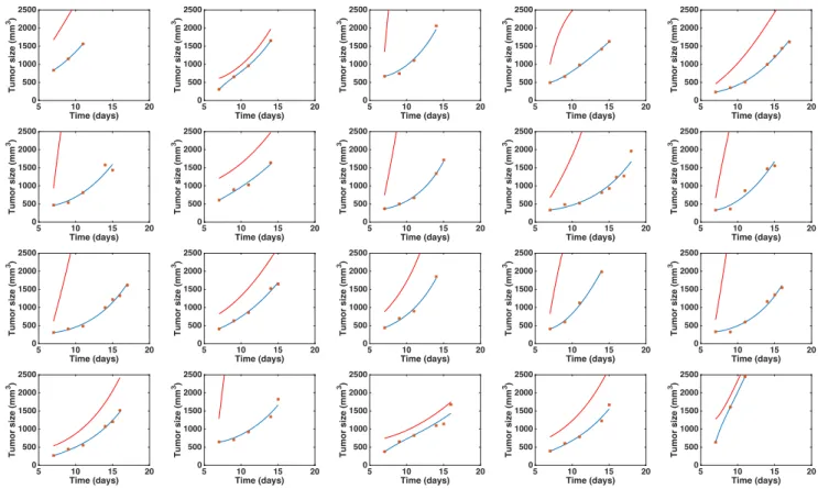
a. Visual inspection of the simulated individual growth curves against the data (Figure 1).

b. Distribution of the (weighted) residuals (all individuals pooled together). It should be gaussian, a hypothesis that can be assessed using the Kolmogorov-Smirnov test (as can be performed using the Matlab function kstest.m) [5]. Two plots of the residuals are outputs when launching launch_fit.m.

c. Computation of the coefficient of determination (R2), defined by

R

2

_{= 1 −}

(

y

i

− f (t

i

)

)

2

∑

y

i

−y

(

)

2

∑

, where yi is the data point at time ti, f(ti) is the solution of the model at this time and

y

is the average of the yi’s. The value of R2 is printed at the screen by launch_fit.m. This number is a usual metric of goodness-of-fit that quantifies how better is the model at explaining the data in comparison to the average only (which would give R2 = 0). The closer R2 is to one, the better the fit.

Time (days) 5 10 15 20 Tumor size (mm 3) 0 500 1000 1500 2000 2500 Time (days) 5 10 15 20 Tumor size (mm 3) 0 500 1000 1500 2000 2500 Time (days) 5 10 15 20 Tumor size (mm 3) 0 500 1000 1500 2000 2500 Time (days) 5 10 15 20 Tumor size (mm 3) 0 500 1000 1500 2000 2500 Time (days) 5 10 15 20 Tumor size (mm 3) 0 500 1000 1500 2000 2500 Time (days) 5 10 15 20 Tumor size (mm 3) 0 500 1000 1500 2000 2500 Time (days) 5 10 15 20 Tumor size (mm 3) 0 500 1000 1500 2000 2500 Time (days) 5 10 15 20 Tumor size (mm 3) 0 500 1000 1500 2000 2500 Time (days) 5 10 15 20 Tumor size (mm 3) 0 500 1000 1500 2000 2500 Time (days) 5 10 15 20 Tumor size (mm 3) 0 500 1000 1500 2000 2500 Time (days) 5 10 15 20 Tumor size (mm 3) 0 500 1000 1500 2000 2500 Time (days) 5 10 15 20 Tumor size (mm 3) 0 500 1000 1500 2000 2500 Time (days) 5 10 15 20 Tumor size (mm 3) 0 500 1000 1500 2000 2500 Time (days) 5 10 15 20 Tumor size (mm 3) 0 500 1000 1500 2000 2500 Time (days) 5 10 15 20 Tumor size (mm 3) 0 500 1000 1500 2000 2500 Time (days) 5 10 15 20 Tumor size (mm 3) 0 500 1000 1500 2000 2500 Time (days) 5 10 15 20 Tumor size (mm 3) 0 500 1000 1500 2000 2500 Time (days) 5 10 15 20 Tumor size (mm 3) 0 500 1000 1500 2000 2500 Time (days) 5 10 15 20 Tumor size (mm 3) 0 500 1000 1500 2000 2500 Time (days) 5 10 15 20 Tumor size (mm 3) 0 500 1000 1500 2000 2500

Figure 1. Individual fits of the tumor growth data by the model for each mouse from one of the two groups. The blue curve is the volume (V) curve while the red curve depicts the dynamics of the carrying capacity (K). Fits were performed by optimization of the coefficients a, b and d. Initial volume V0 was set

to the first volume measured. Initial carrying capacity was set to the double of this quantity. x-axis = time in days, y-axis = tumor size (in mm3).

7. Investigate for statistical differences in the parameters of the model (here a, b, d and

K0) and across the groups under study. File manips_postFitAnalysis.m outputs two things:

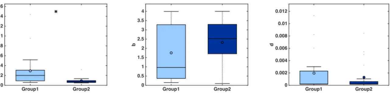
a. Boxplots of the parameter values, including statistical significance (t-test) (Figure 2). Statistical power depends on the number of mice employed. With n = 20 animals, the analysis performed here was able to detect a significant difference of 0.205 day-1 in parameter a between the two groups (0.295 ± 0.0758 in group 1 versus 0.09 ± 0.0132 in group 2, mean ± standard error, see Figure 2), i.e. 69.4%, at the significance level of α = 0.05. To detect a similar difference of 0.2 day-1 _with a probability of success (power) of 95% (i.e., probability of false positive of 5%), only 10 animals are sufficient (and necessary).

Group1 Group2 a 0 0.2 0.4 0.6 0.8 1 1.2 1.4 1.6 Group1 Group2 b 0 0.5 1 1.5 2 2.5 3 3.5 4 Group1 Group2 d 0 0.002 0.004 0.006 0.008 0.01 0.012 1

Figure 2. Boxplots of the distribution of three parameters of the model (a, b and d) for the two groups. Initial condition V0 and carrying capacity K0 were fixed

as in Figure 1. x-axis = Group 1 and Group 2. y-axis = parameter values for a, b and d. * = α < 0.05 (Student’s t-test).

b. Simulated growth curves: either all the animals or averaged other the groups (Figure 3). Time (days) 5 10 15 20 25 Tumor volume (mm 3 ) 0 1000 2000 3000 4000 5000 Time (days) 5 10 15 20 25 30 Tumor volume (mm 3 ) 0 500 1000 1500 2000 2500 3000 3500 Group 1 Group 2 1

Figure 3. Simulated growth curves. Left panel: all individual simulations corresponding to each animal-specific fitted parameter set. Right panel: average growth curves (mean ± standard error). x-axis = time in days, y-axis = tumor volume in mm3. Blue curves = Group 1. Red curves = Group 2.

Acknowledgements

This project was supported, in part, by the National Aeronautics and Space Administration under NSCOR grants NNJ06HA28G and NNX11AK26G and by Award Number U54CA149233 from the National Cancer Institute, both to L. Hlatky. This study also received support within the frame of the LABEX TRAIL, ANR-10-LABX-0057 with financial support from the French State, managed by the French National Research Agency (ANR) in the frame of the “Investments for the future” Programme IdEx (ANR 10-IDEX-03-02).

References

1. Beheshti, A., Benzekry, S., McDonald, J. T., Ma, L., Peluso, M., Hahnfeldt, P. and Hlatky, L. (2015). Host age is a systemic regulator of gene expression impacting cancer progression. Cancer Res 75(6): 1134-1143.

2. Benzekry, S., Lamont, C., Beheshti, A., Tracz, A., Ebos, J. M., Hlatky, L. and Hahnfeldt, P. (2014). Classical mathematical models for description and prediction of experimental tumor growth. PLoS Comput Biol 10(8): e1003800.

3. Hahnfeldt, P., Panigrahy, D., Folkman, J. and Hlatky, L. (1999). Tumor development under angiogenic signaling: a dynamical theory of tumor growth, treatment response, and postvascular dormancy. Cancer Res 59(19): 4770-4775.

4. Ledzewicz, U. and Schattler, H. (2008). Optimal and suboptimal protocols for a class of mathematical models of tumor anti-angiogenesis. J Theor Biol 252(2): 295-312. 5. Massey, F. J., Jr. (1951). The Kolmogorov-Smirnov test for goodness of fit. J Am