Guidance, Navigation, and Control System
for a Dual-Spinning Cubesat
by
MASSACHUSETTS INiTNTE
Evan Dale Wise
OF TECHNOLOGYB.S. Astronautical Engineering
JUL 19 2013
U.S. Air Force Academy, 2011LIBRARIES
SUBMITTED TO THE DEPARTMENT OF AERONAUTICS AND ASTRONAUTICS IN PARTIAL FULFILLMENT OF THE REQUIREMENTS FOR THE DEGREE OF
MASTER OF SCIENCE IN AERONAUTICS AND ASTRONAUTICS
AT THEMASSACHUSETTS INSTITUTE OF TECHNOLOGY
MAY 2013This material is declared a work of the U.S. Government and is not subject to copyright protection in the United States.
Author ... ... .... ... .. .... ... . ...
Department of Aeronautics & Astronautics 23 May 2013
Certified by... ... David W Miller Jerome C. Hunsaker Professor of Aeronautics & Astronautics Thesis Supervisor
A ccepted by ...
Eytan H. Modiano
Associate Professor of Aeronautics & Astronautics Chair, Graduate Program Committee
Guidance, Navigation, and Control System
for a Dual-Spinning Cubesat
by
Evan Dale Wise Submitted to the Department of Aero-nautics and AstroAero-nautics on 24 May 2013
in partial fulfillment of the requirements for the degree of Master of Science in Astronautical Engineering
ABSTRACT
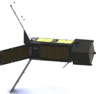
HE MICROSIZED MICROWAVE Atmospheric Satellite (MicroMAS) combines
two traditional control approaches: a dual spinner and a three-axis gyrostat. Unlike typical dual spinners, the purpose of MicroMAS 's 2U bus and spin-ner assembly is to actuate a iu payload, not to add gyroscopic stiffness. An orthogonal triple reaction wheel assembly from Maryland Aerospace, Inc., will both counter the angular momentum from the payload and rotate the satellite's bus about its orbit-normal vector to maintain bus alignment with the orbital frame. The payload spins about the spacecraft velocity axis to scan successive swaths of the Earth. However, the CubeSat form factor restricts the velocity axis to be along the spacecraft minor axis of inertia. This orientation leaves the spacecraft at a gravity-gradient-unstable equilibrium. Further, imperfect can-cellation of the payload's angular momentum induces nutation behavior. An extended Kalman filter is implemented on a 16-bit P1C24 microcontroller to combine gyroscope, limb sensor, and magnetometer data to provide attitude estimation accuracy of approximately 20 arcminutes. Simulations show that the reaction wheels can consistently maintain pointing to within 30 arcminutes for orbits above 40o kilometers with the payload rotating at o.83 hertz.
DISCLAIMER: The views expressed in this thesis are those of the author and do not reflect the official policy or position of the United States Air Force, Depart-ment of Defense, or the U.S. GovernDepart-ment.
Thesis Supervisor: David W Miller
The author would like to thank his family for the support they have provided over the years. He also thanks the MicroMAs team and his stalwart officemates for keeping going when the work seemed overwhelming. He would like to thank his thesis advisor, Prof. David Miller, as well as the principal investiga-tor for the MicroMAS project at the Space Systems Laborainvestiga-tory, Prof. Kerri Ca-hoy, for their support and guidance as he completed his research. This research was conducted under an M.I.T. contract with Lincoln Laboratory, number PO 7000180248.
Introduction
1.1 Motivatio 1.2Backgrou
1.3 Literature 1.3.1 Cubes 1.3.2 Dual-1.3.3 Attitu 1.4 Requirem 1.5 Concepto 13 n 13 nd 13 Review ats 15 Spinners de Estimation ents 16fOperations
2Attitude Dynamics
19 2.1 Reference Frames 192.1.1 The Inertial Frame 20
2.1.2 The Earth-Fixed Frame 21
2.1.3 The Body-Fixed Frame 22
2.1.4 The Orbital Frame 22
2.2 Equations of Motion 23
2.2.1 Euler's Moment Equations 23
2.2.2 Rotation Matrices and Relative Angular Velocities
2.3 Why a Simple Spinner Will Not Work 26
2.3.1 Slewing via an External Torque 26
2.3.2 Constant, Nonzero System Angular Momentum
15 5 16 17 25 27
Dual-Spinner Dynamics 28
Slewing via an External Torque 29
Constant, Nonzero System Angular Momentum
Zero-Angular-Momentum System 34
Linear Stability Analysis 34
Wobble 35
dware
37
2.4 2.4.1 2.4.2 2.5 2.5.1 2.5.2Har
3.1 3.1.1 3.1.2 3.1.3 3.2 3.2.1 3.2.2 3.2.3 3.2.4 3.2.5 3.2.6 3.34
Estimation and Control Approach
4.1 Position Estimation 45
4.1.1 Propagation Methods 45
4.1.2 Practical Considerations 46
4.2 Attitude Estimation 47
4.2.1 Review of Extended Kalman Filter
4.2.2 Attitude Parameterizations 48
4.2.3 Propagation 49
4.2.4 Update 52
4.2.5 Square Root and Factored Forms
31 39 40 to the GNC System
45
47 53 8 Actuators 37 Reaction Wheels 37Magnetic Torque Rods 37
Scanner Assembly Motor 38
Sensors 38
GPS and Why We Aren't Using It
Sun Sensors 39
Magnetic Field Measurement Earth Limb Detection 42
Inertial Measurement Unit 43
Scanner Assembly Encoder 43
4.3 Attitude Control
5
Simulation
57
5.1 Design 57 5.1.1 Dynamics 5; 5.1.2 Models Used 5.2 Results 59 5.2.1 Detumbling 5.2.2 Slew 59 5.2.3 Stabilization 5.3 Sensitivity Analysis 5.3.1 5.3.2 5.3.3 5.3.4 54 58 59 6o 64Scanner Assembly Rotor Bearing Axis Misalignment Gyro Axis Misalignment 64
Magnetometer Misalignment 66
Static Earth Sensor Misalignment 66
6
Testing
71
6.1 Introduction6.1.1
Backgrou 6.1.2 Test Item 6.1.3 Test Obje 6.1.4 Limitatio 6.1-5 Test Reso 6.2 Test and Eva6.2.1 General 6.2.2 Objective 6.2.3 Mission S
Conclusions
79
70.4 Novel Work 70.5 Future Work 72 nd 72 Description 72 ctives 72 ns 73 urces 74 luation 74 Test Objectives 75 1: Detumbling Mode uitability 77 79 79 64 757
MicroMAS 14
Orbit Track and Swath Overlap 14
Precession of the Equinoxes and Nutation of the Poles 20 The Body-Fixed Frame 22
The Local Vertical-Local Horizontal Frame 22
MicroMAs As a Simple Spinner 26
MicroMAs Maintaining LVLH Alignment with Constant Momentum 27 Momentum Trading Between Two Orthogonal Reaction Wheels at Each Quarter Cycle (Clockwise) 28
MicroMAs as a Partially-Despun Dual Spinner. 29 Reaction Wheel Required Speeds and Torques 32
MicroMAs as a Zero-Angular-Momentum System 34
Unbalanced Spacecraft Geometry 36
3.1 Attitude Sensor Locations on MicroMAS 38
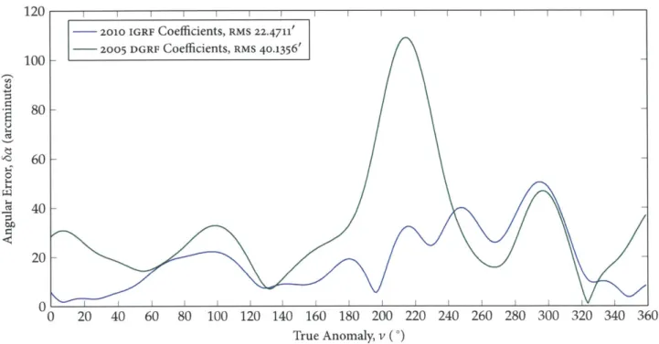
3.2 Relative Rotation Sensor Locations on MicroMAs 3.3 Angular Error of Sixth-Order/Degree IGRF Model vs.
IGRF Model 41
3.4 The Voyager Spacecraft 42
39
Thirteenth-Order/Degree
4.1 General Estimation Architecture: Complementary Feedback 5.1 Detumbling Control History and Angular Rate Trajectory 5.2 Slew Mode Angle and Rate Trajectory 6o
5.3 Slew Mode Control History 61
5.4 Slew Mode Disturbance Torques 61
5.5 Stabilization Mode Angle and Rate Trajectory 62 5.6 Stabilization Mode Angular Error 62
5.7 Stabilization Mode Control History 63 5.8 Stabilization Mode Bias Error Estimate 64
5.9 RMs Pointing Error Due to Varying Rotor Bearing Axis Misali
1.1 1.2 2.1 2.2 2.3 2.4 2.5 2.6 2.7 2.8 2.9 2.10 52 59 gnment
12
5.10 RMs Reaction Wheel Speed Increase Due to Varying Rotor Bearing Axis Misalignment 65
5.11 RMs Pointing Error Due to Varying Gyro Misalignment 66
5.12 RMs Reaction Wheel Speed Increase Due to Varying Gyro Misalignment 67 5.13 RMs Pointing Error Due to Varying Magnetometer Misalignment 67 5.14 RMs Reaction Wheel Speed Increase Due to Varying Magnetometer
Mis-alignment 68
5.15 RMs Pointing Error Due to Varying Cross-Track Static Earth Sensor Mis-alignment 68
5.16 RMs Reaction Wheel Speed Increase Due to Varying Cross-Track Static Earth Sensor Misalignment 69
5.17 RMs Pointing Error Due to Varying Anti-Ram Static Earth Sensor Mis-alignment 69
5.18 RMs Reaction Wheel Speed Increase Due to Varying Anti-Ram Static Earth Sensor Misalignment 70
6.1 MicroMAS ADCs Test Platform 71 6.2 Radiometer Payload Inertia Mockup 72
6.3 Linear Stage Mass Adjusters from the Crowell Testbed 72
6.4 MicroMAs Test Avionics Stack 73 6.5 3-DoF Hemispherical Air Bearing 74
6.6 3-DoF Air Bearing and 3-DoF Helmholtz Cage and Drivers 74
1
INTRODUCTION
1.1 MOTIVATION
HE LITERATURE IS rife with ideas for new filters and sensor models for
em-bedded systems, but there is little floating around that actually discusses practical selection and implementation of these things on an very small spacecraft. Most such papers that do exist deal with spacecraft of entirely differ-ent form factors than the small satellites preferred by universities today.' Cube-sats have neither the flight heritage nor component availability of larger space-craft. So while the reader may not find any new groundbreaking theories of estimation or control, the reader will find a useful synthesis of estimation and control design for processor-limited embedded systems with limited sensor and actuator choices. The thesis is intended to be a combination survey paper, de-sign document, and record of success and failure.
This paper is targeted specifically at newcomers to the Space Systems Labo-ratory and more generally at students interested in ADCS for small spacecraft, specifically for spacecraft with limited, embedded computing.
1
Tisa and Vergez, Performance Analysisof Control Algorithms for FalconSat-3;
S. Andrews and Morgenstern, Design,
implementation, testing, andflight results of the TRMM Kalman filter.
1.2 BACKGROUND
The Micro-sized Microwave Atmospheric Satellite (MicroMAS) combines two traditional spacecraft control problems: that of a dual spinner and a three-axis gyrostat. Because the scanner assembly, which contains a microwave radiome-ter for the purposes of all-weather atmospheric sounding,2 makes up a com-paratively large portion of the spacecraft's mass, it effectively becomes a large rotor such as would be found on a traditional geostationary communications satellite such as INTELSAT iv or the Japanese cs and CS2. Unlike traditional dual spinners, however, the purpose of MicroMAS 's spinner is not to add gyroscopic stiffness.
Rather than for the traditional motivation of added stability, MicroMAS 'S arrangement is due to the size limitations of the CubeSat form factor: the ro-tational motion of the scanner allows it to scan the field of view of the payload over adjacent swaths of the Earth's surface and space while the translational
mo-2 Blackwell et al., "Improved all-weather atmospheric sounding using hyperspectral microwave observations".
14 DESIGN, ANALYSIS, & TESTING OF A PRECISION GNC SYSTEM FOR A DUAL-SPINNING CUBESAT
Figure 1.1: MicroMAs
-V
tion of the satellite through its orbit provides the advancement from swath to swath (see Figure 1.2).
Figure 1.2: Orbit Track and Swath Overlap
Because the payload must be oriented to rotate about the orbital velocity vector throughout the orbit (see Figure 1.2), reaction wheels are needed to both counter the angular momentum from the payload (keeping the bus portion of the spacecraft stationary in the orbital frame) and spin the satellite about its orbit-normal vector to keep the antenna pointing nadir and the payload imag-ing at nadir.
MicroMAs has three reaction wheels each aligned with a principal axis, a three-axis microelectromechanical system (MEMS) rate gyroscope, two sets of thermopile static Earth limb sensors, a triaxial magnetometer, six coarse sun sensors, and a motor with an optical encoder to rotate the scanner assembly. The reaction wheel assembly, an MAI-400 model, was purchased from Mary-land Aerospace, Incorporated, and includes the static Earth sensors as well as a small ARM processor that can accomplish some basic estimation and control tasks. The sun sensors consist of simple photodiodes mounted on six outward
faces of the spacecraft. Most of the spacecraft's estimation and control will be ac-complished aboard the spacecraft's primary flight computer, a 16-bit Microchip PIC24 microcontroller. Each of the reaction wheels can be commanded for an-gular velocity and torque. The rate gyro can determine rotational velocities in all three body axes. The two infrared static Earth sensors between them can de-termine the nadir vector. The sun sensors can roughly dede-termine the sun vector when the spacecraft is not in eclipse.
MicroMAs has been designed to a nominal orbit with an inclination of 40 degrees and an altitude of Soo kilometers.
1.3 LITERATURE REVIEW
1.3.1 Cubesats
A cubesat is a satellite form factor developed at California Polytechnic in an attempt to standardize university small satellites and stimulate a market to de-velop commercial, off the shelf COTS options for satellite design. Previous cube-sats have used massive means of attitude control; a popular solution is perma-nent magnets to align the satellites with the Earth's magnetic field. The Univer-sity of Michigan's Radio Aurora Explorer (RAX) uses this option.3 Spacecraft with tighter pointing requirements have used electromagnets. Only recently has technology miniaturization caught up to allow cubesats to employ momentum exchange devices such as reaction wheels. The ExoplanetSat spacecraft uses a two-stage controller with reaction wheels for coarse pointing and a piezoelec-tric translational stage to position the optics for fine pointing.4 Another project called Mothercube uses MEMs electrospray thrusters for individual spacecraft attitude control and multiple spacecraft formation control.
I Springmann et al., "The attitude
determi-nation system of the RAX satellite".
4 Pong et al., High-Precision Pointing and
Attitude Determination and Control on ExoplanetSat.
1.3.2 Dual-Spinners
Traditional spinning spacecraft were used for communications. The addition of a despun platform resulted in what is called a "dual-spinner" design. A sig-nificant amount of work was done in the 196os and 1970s with dual-spinner dynamics.5 More recent work has examined system damping due to structural flexibility.6 The problem is that all of these papers orient the rotor either with the pitch axis of the spacecraft or with an arbitrary intertial pointing direction, which makes sense when taking advantage of gyroscopic stiffness, but does not
correspond to MicroMAs's arrangement. None of the nadir-pointing
configura-tions studied mounted the spinner in the along-track direction.
Communications satellite companies examined problems with spinner bal-ancing in the late 1960s and early 1970s. At Hughes, McIntyre and Gianelli dealt with the wobble that results from imperfectly aligned principal axes of inertia and rotation axes. They describe an exact solution for a platform that is sym-metric about the axis of rotation and approximate solutions for.7 At Telesat Canada, Wright proposed a system of movable masses for altering the balance
I See, for example, Likins, "Attitude sta-bility criteria for dual spin spacecraft"; Phillips, "Linearization of the Closed-Loop Dynamics of a Dual-Spin Spacecraft".
6 Ortiz, "Evaluation of energy-sink stability
criteria for dual-spin spacecraft".
7 McIntyre and Gianelli, "Bearing axis
16 DESIGN, ANALYSIS, & TESTING OF A PRECISION GNC SYSTEM FOR A DUAL-SPINNING CUBESAT
'Wright, "Wobble Correc-tion for a Dual-Spin Vehicle".
9 Bill Widnall, personal conversa-tion, 14 March 2013; Don Eyles,
per-sonal conversation, 9 April 2013;
and Mindell, Digital Apollo, p. 103.
Murrell, Precision attitude
deter-minationfor multimission spacecraft.
"Lefferts, Markley, and Shuster, Kalman
Filteringfor Spacecraft Attitude Estimation.
" Crassidis and Junkins, Optimal
esti-mation of dynamic systems, pp. 457-60. 1 Markley, "Matrix and
Vector Algebra", p. 755. 4 S. Andrews and Morgenstern, Design,
implementation, testing, andflight re-sults of the TRMM Kalman filter; S. F.
Andrews, Bilanow, and F. Bauer, Recent
Flight Results of the TRMM Kalman Filter.
" Wahba, "A Least Squares Es-timate of Satellite Attitude". An overview of the main forms of these methods is available in Markley and Mor-tari, How to Estimate Attitudefrom Vector
Observations; Bar-Itzhack and Oshman,
"Attitude Determination from Vector Observations", See also; Markley and Mortari, "New Developments in
Quater-nion Estimation from Vector Observa-tions"; Markley and F. H. Bauer,
Space-craft Attitude Determination Methods;
and Markley, "Optimal Attitude Ma-trix from Two Vector Measurements".
1 tangyin-many_2007.
"Natanson and Glickman, A Study
of TRMM Static Earth Sensor Perfor-mance Using On-Orbit Sensor Data.
of the rotor on orbit.8
1.3.3 Attitude Estimation
Recursive least-squares estimation has a long history with spaceflight. The Apollo Guidance Computer used a variation of a square-root information filter for atti-tude determination, updating gyro biases with angles measured from pointable optical telescopes.9 The Multimission Modular Spacecraft (MMS) demonstrated several advances in quaternion estimation in 1978,10 and its primary Kalman fil-ter algorithm was summarized and explained by Lefferts, Markley, and Schusfil-ter in 1982.11
This ADCS used an inertial measurement unit IMU, with two star trackers and a fine sun sensor to update the integrated angle errors and gyro biases. The MMS used a first-order quaternion propagation with a 256-millisecond timestep. Crassidis and Junkins extended the algorithm to the discrete-discrete case in their book12
using the power series approach given by Markley.13 This type of
filter (and in fact the same software) was subsequently used in the Rossi X-Ray Timing Explorer and thence adapted for the Tropical Rainfall Measuring Mis-sion (TRMM) for use with a triaxial magnetometer and additional sun sensor.14 The Triaxial Attitude Determination (TRIAD) method was first developed at the Applied Physics Laboratory and published in 1964 for combining a solar vector measurement with another vector measurement. When Grace Wahba posed her eponymous least-squares single-frame attitude estimation problem in 1965,15 interest exploded in attitude determination methods, and many vari-ations of many methods were developed to combine attitude information.16 Tangyin and Shuster summarize the different variations of the TRIAD method.17 In addition to the sun sensor-magnetometer extended Kalman filter, the TRMM also has an alternative attitude determination mode that uses four static Earth sensors and two digital Sun sensors.8 It uses a more optimal method than TRIAD to combine the measurements, but results should be analogous to
MicroMAs.
1.4 REQUIREMENTS
The geolocation requirement for MicroMAS 's payload data is that the total ge-olocation error of the observations shall be less than 30 percent of the effective pixel diameter (io percent goal). Since the beamwidth of the spacecraft's pay-load is 2.4 degrees, this effectively translates to an error of less than 14.4 arcmin-utes goal (0.24 degrees) and 43.2 arcminutes threshold (0.72 degrees).
Given the errors introduced from timing and the scanner assembly encoder, the ADCS is left with a threshold requirement of 30 arcminutes pointing knowl-edge with a goal of io arcminutes, and a threshold requirement for pointing of 6o arcminutes with a goal of 30 arcminutes.
eclipse, so the spacecraft cannot rely on sun sensors for precise attitude deter-mination. While it is possible to rely on gyro propagation during the period of eclipse, the sorts of gyros with the drift rates that could handle the required precision are far outside the budget of MicroMAS. Thus, the spacecraft must rely on other celestial reference points, such as the stars or Earth.
1.5 CONCEPT OF OPERATIONS
After launch, the spacecraft will deploy from a Poly-Picosatellite Orbital De-ployer (P-POD), wait thirty minutes, and use a nichrome burn wire to release the deployable solar panels and monopole antenna. Then the spacecraft will enter the detumbling mode, using a B-dot controller to damp the spacecraft's angular rotation. When the spacecraft has slowed to within the angular rate of change of the geomagnetic field, the spacecraft will enter its slew mode, where it will use its magnetometer and coarse sun sensors to determine attitude and the reaction wheels to slew to align itself with the local-vertical, local-horizontal (LVLH) frame. When the limb is in the field of view of the static Earth sensors, the spacecraft will switch to stabilization mode, spin up the scanner assembly, and begin collecting data with the payload.
(<
-p6 T & -u Totafra AsyeTat, 6ua a"T& &nep biv tispwv Elvat Asyeai,, 6rwoofiv &ikw npos &repov.... t'i & xai rotafra T6v irp6c Ti olov ili4, 8idA6eori, air6qaIt, s7s pq, 6sart(. n71va yap Ta eipqpsva afti
&nep sqlv ftspwv elvat AtyCet xal on I o n.X T' yA yap Ttv6 yost
AsyeTaI xai q emovrTpy tvo EtIqy xai 6sats T vk Oioriq, xai t Wa
U (boraftw . >
(
Those things are called relative, which, being either said to be of something else or related to something else, are explained by reference to that other thing.... There are, moreover, other relatives, e.g. habit, disposition, perception, knowledge, and attitude. The significance of all these is explained by a reference to something else and in no other way. Thus, a habit is a habit of something, knowledge is knowledge of something, attitude is the attitude of something. So it is with all other relatives that have been mentioned.)
-Aristotle', Categories
'trans. E.N. Edgehill, Oxon., 1928; emphasis added by the author. It is interesting to note
NALYSIS OF THE SPACECRAFT s dynamics allows for a more educated design that Osorg, the Greek word for attitude or of ADCs architecture and thus eases the component selection process. The position, is the same word thesis that has come to mean an academic stance and the danalyses
in this chapter also provide a basis to which we can relate subse- discussion supporting such. quent simulation and test results.
2.1 REFERENCE FRAMES
As Aristotle noted above, for the attitude of one object to make sense, it must be compared against the attitude of some other object. In the case of an Earth-observing spacecraft, that "something else" is usually the Earth; and so we must define how we are measuring the orientation of the Earth's reference frame as well as the orientation of the spacecraft's reference frame. Additionally, since Newton requires an inertial reference frame for us to use calculus properly, we must determine the orientation of the inertial reference frame relative to the Earth's reference frame.
20 DESIGN, ANALYSIS, & TESTING OF A PRECISION GNC SYSTEM FOR A DUAL-SPINNING CUBESAT
2.1.1 The Inertial Frame
2 In antiquity, this vector pointed to the
star y Arietis (proper name Mesarthim), in the constellation Aries. Because of this alignment, the vernal equinox di-rection is frequently represented by the astrological symbol for the constella-tion Aries, the ram's head Y. Because of equinoctial precession, this vector moved into Pisces X around 70 BC. Regardless, the vernal equinox direction is still fre-quently called the first point of Aries.
Bate, Mueller, and White,
Funda-mentals of astrodynamics, p. 105.
, Pole
vernal equinox T shifts westward
Figure 2.1: Precession of the Equinoxes and Nutation of the Poles. Adapted from Figure 2.9-2 of Bate, Mueller, and White,
Fundamentals of astrodynamics, p. 105. 4 This mean-of-date frame used less
pre-cise precession and nutation models from today. It was originally adopted
un-der the IAU'S 1976 resolutions and subse-quently modified to use the Fifth Funda-mental Catalog (FK5) of celestial objects as fiducial points to define the system.
I Vallado and McClain,
Fundamen-tals ofAstrodynamics and Applications,
p. 16o; The Astronomical Almanac, B25.
The geocentric equatorial reference system (commonly called simply "IJK") at first examination seems simple: it is centered at the Earth's center (i.e., geocen-tric) and has a fundamental plane aligned with the Earth's equator (i.e., equato-rial). Because of this positioning, it is also known as the Earth-centered inertial (ECI) frame. Its primary axis, along
f,
passes through the equator to point at the Sun during the northern hemisphere's vernal equinox (the first day of spring, wherein the lengths of day and night are equal)-this line also corresponds with the intersection of the Earth's equatorial plane and the ecliptic plane.2Its second direction,
J,
is normal to the first, similarly passing through the equa-tor, and its third direction, K, is oriented along with the geographic north pole, forming a dextral, orthonormal system.Contention arises when considering that the traditionally-defined geocen-tric equatorial frame is not, in fact, inertial. The equatorial plane of the Earth is tilted 23.5 degrees relative to the ecliptic plane, causing the equinox to pre-cess; the Earth's polar axis sweeps out the shape of a cone similar to a wobbling top. The period of this motion is about 26,ooo years. Additionally, tidal forces from the moon add an additional perturbation, causing a nutation of the Earth's
motion with a period of 18.6 years.3 This motion is illustrated in Figure 2.1.
The traditional way to account for this effect in astronomical observations is to refer to the locations of the mean equinox and equatorial plane within a cer-tain duration from a particular time, or epoch; astrodynamicists can achieve a
pseudo-inertial frame close enough to a Newtonian inertial system for practical use. This resulting approximation of the equinox at a particular epoch is called a mean-of-date system. The most recent frame of this sort was under the
IAU-76/FK5 reference system, using the J2000 epoch (i.e., the location of the mean equator and equinoxes on 1.5 January AD 2000).4
The currently accepted geocentric inertial coordinate frame of the Interna-tional Astronomical Union (IAu) is the Geocentric Celestial Reference Frame (GCRF), adopted with the IAU 2000 resolutions.5 Its axes correspond closely
to the those from the previously accepted IAU-76/FK5 system with the J2000 mean equator and equinox, though it is far "more inertial": the GCRF's axes are time-independent and aligned with the International Celestial Reference Frame (ICRF) radio source catalog with its primary axis aligned with a stationary extra-galactic radio source, 3C 273, rather than the changing equatorial plane.
For analytical purposes, the mean-of-date system with the epoch at launch should be sufficient, since it results in errors of only arcminutes over the one-year design lifetime of MicroMAS, which is an order of magnitude smaller than the attitude determination requirements. For precision work, such as for pre-cision orbit determination to geolocate the payload data, the GCRF should be used.
Planetary and stellar ephemerides are described in this reference frame. Ab-breviated mean-of-date analytical models are accurate to within an arcminute
for the Sun6 (used aboard the spacecraft for attitude determination), and 18 ar-cminutes for the Moon7 (useful for modelling third-body gravitational effects and albedo but not necessary for attitude determination). The most accurate ephemerides are compiled by the Jet Propulsion Laboratory from observational data and are specifically based in a solar-system barycentric form of the ICRF.
The DE405 ephemerides are those used for the Astronomical Almanac, and are
precise to within about i milliarcsecond for the the inner planets and 1oo
mil-liarcseconds for the outer planets8-this precision is completely unnecessary for any precision orbit determination modelling or attitude modelling for
Mi-crOMAS.
Because this reference frame is inertial, it is the one with respect to which changing quantities are differentiated and integrated.
6 The Astronomical Almanac, c5; Vallado
and McClain, Fundamentals of
Astrodynam-ics and Applications, pp. 279-80.
7The Astronomical Almanac, D22; Vallado and McClain, Fundamentals of
Astrodynam-ics and Applications, p. 289.
6 Standish, JPL Planetary and Lunar
Ephemerides, DE405/LE405.
2.1.2 The Earth-Fixed Frame
While similar to the ECI frame, the Earth-centered, Earth-fixed (ECEF) frame rotates with the Earth rather than remaining fixed in inertial space. Under the mean-of-date system, the transformation between the ECI frame and the ECEF
is a single rotation based on the elapsed time and the mean rotation rate of the Earth. Such a rotation does not account for nutation, precession, or polar motion of the Earth, which can cause errors on the order of tens of kilometers in low Earth orbit.9
The International Terrestrial Reference Frame (ITRF2008) is the IAU'S terres-trial frame of choice and is periodically updated based on changes in monitor-ing station locations due to plate tectonics. The U.S. Department of Defense prefers the wGs-84 terrestrial system, which bases its definition on measure-ments through the Global Positioning System (GPS). Over the years that the
ITRF and WGS-84 have been in use, measurement methods (including GPS posi-tioning of the groundstation locations) have converged such that negligible dif-ference (centimeters at Earth's surface) exists between the two systems.14 With the divorce of the GCRF from an equatorial basis, a more involved transforma-tion must account for the precession and nutatransforma-tion of the Earth through Earth
orientation parameters (EOPs) in addition to the instantaneous time at the prime meridian (a function of terrestrial time, rather than universal time).
Analysis performed at U.C. Boulder suggests that for positional accuracy on the order of hundreds of meters at LEO, the transformation between the GCRF
and ITRF, no EOPs need be used; for accuracy on the order of tens of meters at LEO, only the difference between universal time and coordinated universal time need be accounted for."
Earth atmospheric, magnetospheric, and gravity models are all described in this reference frame.
9 Bradley et al., Earth Orientation Parameter
Considerations for Precise Spacecraft Operations.
The Astronomical Almanac, K13.
Bradley et al., Earth Orientation
Param-eter Considerations for Precise Spacecraft Operations.
22 DESIGN, ANALYSIS, & TESTING OF A PRECISION GNC SYSTEM FOR A DUAL-SPINNING CUBESAT
2
Figure 2.2: The Body-Fixed Fr
Figure 2.3: The Local Verti-cal-Local Horizontal Frame
Vallado and McClain, Fundamentals of
Astrodynamics and Applications, p. 163. 13 Kuipers, Quaternions and Rotation Sequences, p. 84.
4 Wie, Space vehicle
dy-namics and control, p. 388. '5 Wie, Space vehicle dynamics and control,
p. 365; Markley, "Equations of Motion".
2.1.3 The Body-Fixed Frame
Another set of unit vectors
(2,y
,2
constitutes the basis for the body-fixed ref-erence frame 9~, centered at the center of mass of the spacecraft. The pri-mary axis corresponds to the long axis of the spacecraft, the minor axis of in-ertia, which should nominally be in the ram, or velocity; direction; the second axis corresponds to the nominal cross-track direction; and the third axis corre-sponds to the nominal nadir direction (see Figure 2.2).Ideally, this reference frame would be aligned with the principal axes of the spacecraft, i.e., those axes for which the principal moments of inertia are the di-agonal of the inertia tensor and the coupled products of inertia are zero. How-ever, designing the structure requires fitting often oddly-shaped components ame into a limited area, unevenly distributing the mass across the spacecraft's cross section, and leaving these products of inertia with small, nonzero values. Small trim masses can mitigate this effect, but not entirely remove it. Thus, there is a small rotation between the geometric body frame, to which the sensors and actuators are (nominally) aligned, and the principal axis body frame, to which the mass is aligned. Preliminary analysis will consider the two body frames to be equivalent.
2.1.4 The Orbital Frame
The orbital along-track reference frame with unit vectors
(k,
g,NI
travels with the spacecraft like the body frame, but rotates based on the spacecraft's orbital characteristics. Its primary directionA
is in the radial direction from the center of the Earth to the satellite,S
is the along-track axis-perpendicular to the radial axis, and parallel to the velocity axis for circular orbits-andNJ
is normal to theorbital plane (see Figure 2-3).
The orbital frame is often called the "local vertical-local horizontal" (LVLH) frame because of this satellite-fixed, directional basis. A commonly used variant of the LVLH frame is the roll-pitch-yaw coordinate system (RPY). The roll axis is the same as the $ axis of the along-track system, the yaw axis is opposite the position vector R (i.e., it points nadir), and the pitch axis is opposite the angu-lar momentum vector of the orbit. Because of the more intuitive nature of the RPY reference frame (analogous to the wind-axis reference frame used in avi-ation), the spacecraft's attitude maneuvers can be described between the body frame and the LVLH frame using a 3-2-1 Euler-axis rotation sequence with Euler angles that measure bank angle ((P), elevation (0), and heading (V)).12 Perturba-tions from the nominal orientation are called roll (64), pitch(60), and yaw (64'). Kuipers calls this 3-2-1 sequence the Aerospace Sequence,13 and Wie prefers it when discussing LVLH maneuvers and derivations.14 The 3-1-3 sequence is also popular for spacecraft applications, especially for spinning spacecraft and in-ertial pointing systems that do not consider a local vertical-local horizontal frame.'5 Since MicroMAs is nominally aligned with the LVLH frame, we will stick to the Aerospace Sequence.
2.2 EQUATIONS OF MOTION
This section will derive the equations of motion for the most complex satellite design considered for MicroMAS, i.e., a dual-spinning spacecraft with three ad-ditional orthogonally-mounted reaction wheels. The subsequent analysis sec-tions will use simplified versions of the equasec-tions of motion, removing terms as components are removed.
These investigations will use the MAI-40o reaction wheel set as a function-ally representative example of available cubesat-sized momentum storage de-vices. Chapter 3 will examine commercial options for such devices in greater detail. The spacecraft's payload and reaction wheels are assumed to be perfectly axisymmetric. The principal axis system is assumed to align with the geometric axis system.
2.2.1 Euler's Moment Equations
The first principle from which our equations of motion will be developed is the rotational analogue of Newton's second law:
- (I' = Text (2.1)
dt
Since the rotating reference frame, the body frame, is determined based on the rotation of the spacecraft's bus, the angular velocity of the bus IB is equal to that of the angular velocity of the body frame with respect to the inertial frame, i.e.,
2B
= i/1. The MicroMAs spacecraft itself has five individual but connected components that contribute to its angular momentum: the LVLH-stationary bus, HB; the three reaction wheels, HRW. for i = 1,2,3; and the rotating payload,HPL. Thus
3
H = B + HPL + f1RW (2.2)
i=1
For ease of notation, we will write the sum 1 RWi as simply NRW. If we as-sume each reaction wheel is perfectly orthogonal to the others, then each com-ponent of HRW can be thought to represent the angular momentum of each reaction wheel.
Equation 2.3 below explains the derivative of the left-hand side of Equation 2.1 in the spacecraft's body reference frame. Note the Coriolis term taking into ac-count the rotation of the body frame.
d d _B/ j4
-1 1
N
d-.+B/. x, (2.3)dt dt
Again for ease of notation, and to save space, we will write time derivatives with respect to the body frame-that is in Leibniz notation, A B, where-is some generic vector-as an overhead dot in Newton notation: Substituting
Equa-24 DESIGN, ANALYSIS, & TESTING OF A PRECISION GNC SYSTEM FOR A DUAL-SPINNING CUBESAT
tion 2.3 into Equation 2.1 yields
HB + HPL + HRW + RB/I X (1B + HPL + HRW) = iext
HB + HPL + HRW + 3BI X HB + B/I X PL + 6B X IRW = (2.4)
The angular momentum of an object is given by
Nf
=f
- i;,(2.5)where
f
is the inertia dyadic of the object; the time derivative of the angular momentum is thusH = J - + (2.6)
Since we are assuming that the reaction wheels and payload are axisymmetric, their inertia dyadics JRW and 4PL do not change during operation. The only inertia dyadic in the system that will change is that of the bus when the solar panels deploy. Since we are examining nominal operation, we can ignore this
'B term as well. Substituting Equations 2.5 and 2.6 into Equation 2.4 yields the vector form of Euler's moment equation for our spacecraft:
IB
. B/I + !PL ' PL + jRW 'RW + 1B/IX B .g
B/I + OB/I X JPL ' PL + XJRW ' RW =ext (2.7)-B/Iwhere the payload and reaction wheel angular velocities ('DPL and &RW) contain the angular motion of the body frame )B/I as well as their own motions relative to the body frame (dPL and ORW):
PL =BI + PL (2.8a)
WRW = B/I + RW (2.8b)
Since the angular momentum term derivatives
ORW
andOPL
were differenti-ated with respect to the body frame, we can treat them as internal torques ap-plied to the spacecraft body by the wheels ERw and spinning payload iPL. If we additionally let I = jB +JPL +JRW and substitute Equations 2.8 into Equation 2.7, this reduces to/ -B + ID"/ X / - B/l + iPL + ' B/I X jPL'PL +i RW + g RX /RW 'RW Zx 29
System Terms Payload Terms Reaction wheel Terms
16 In a given frame F, the inertia ten- Since we assumed the principal axis frame aligns with the geometric frame, the
sor (also called inertia matrix) of inertia tensor expressed in the body frame16
for each part of the system should a body JF is related to the inertia be diagonal, i.e., J = diag X We can thus write Equation 2.9 in matrix dyadic of that body j by the relation
= fTjFf form as a system of Euler's equations of motion, describing rotations about each
of the spacecraft's principal axes: Textx Ix x Texty = Jyy L Textz I JZz A External Torques +
[
Whole T1Iz
- jy y TPL 0 TRW1
(I -Jz) aoxOz + 0 + JPLOPLOz + TRW y y Ox6y]x
0 -JPLOPLCy TRWzSpacecraft Payload Spinner
'erms Terms
(2.10)
+
JRW (URWzWy - ORWy6z) JRW (ORW,6z - ORWz 6ox)
JRW (ORWY WX - DRWXW
Jy
Reaction Wheel Terms
2.2.2 Rotation Matrices and Relative Angular Velocities
An analysis of MicroMAS's pointing depends upon the spacecraft's alignment with the local vertical-local horizontal frame. We can use the Aerospace Se-quence to get the Euler angles between the spacecraft body frame and the LVLH
frame:
cos cos V5 cos0sin4' -sin0
CBIO sin sin0cosip-cosPsin4p sinesin0sin4i'+cos cos V) sin cos0
cosqsin0cosV'+sinqsin4 cos sin0sin i-sinPcosip costPcos0
(2.11) We can describe the spacecraft's motion relative to the orbital frame by the rela-tion
B/I -_ B/O + E0/I (2.12)
where, for a circular orbit, the orbital reference frame's angular velocity relative to the inertial frame is simply -n02, the mean motion of the orbit, which is equivalent to the instantaneous angular velocity over all of the circular orbit. This quantity is
n = (2.13)
where ye is the gravitational constant for the Earth and a is the orbit's semimajor axis (which is the radius for circular orbits). For a 50o-kilometer orbit, this quantity amounts to 398,600.5 km 3 n = -N (6,378.137 km + 500 km)3 = 1.1068
-The components of JB/O from Equation 2.12 can be expressed in the body frame
as
CVB/O =
(4
+ Rot (0)6 + Rot1 (#)Rot2(A))[1 0
-sin
01
1
0
cos4 sin cos0l 1
0 - sin$0 cos 0cos 0
26 DESIGN, ANALYSIS, & TESTING OF A PRECISION GNC SYSTEM FOR A DUAL-SPINNING CUBESAT
and so the components of angular velocity of the body frame with respect to the inertial frame expressed in the body frame are
0 wB/I - wB/0 - nCB/O 1 0
1 0 -sin0 cos0sin4
1
0 cos# sinucos 0 n sin sin0sinip+cospcos4' (2.15)
0 -sin P cosp0cos 0 cos sin 0sin@p- sin P cos
p.
For our linear stability analyses, we really only care about small perturbational angles 6b, 60, 64, and small perturbational rates 64, 60, 64. We can thus linearize the relationships between the reference frames using the small angle assumption and ignoring higher-order terms. Equation 2.11 becomes
1 64' -60
CB/O
[
-64 1 6p (2.16)60 -6b 1
and Equation 2.15 becomes
o0 _ b0 - nbip (2.17a)
og y 60 - n (2.17b)
6oz
- 4 + nbo (2.17c)
Assuming we are also dealing with small perturbational angular accelerations, we can find the time derivatives of Equations 2.17 as
6 - n6o (2.18a)
6
y (2.18b)
z b + n6o it (2.18c)
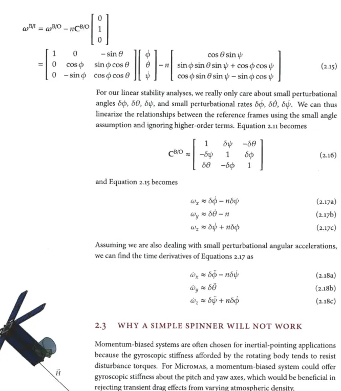
2.3 WHY A SIMPLE SPINNER WILL NOT WORK
Momentum-biased systems are often chosen for inertial-pointing applications because the gyroscopic stiffness afforded by the rotating body tends to resist disturbance torques. For MicroMAS, a momentum-biased system could offer
H gyroscopic stiffness about the pitch and yaw axes, which would be beneficial in
rejecting transient drag effects from varying atmospheric density. Figure 2.4: MicroMAs As a Simple Spinner 2.3.1 Slewing via an External Torque
Moving the angular momentum of the system requires an external torque (called
17'This type of precession is different "precession";17 see Equation 2.1).
To maintain the spacecraft's alignment with from precession usually discussed in the LVLH frame, we would need to slew at a rate equal to the angular velocity
classical mechanics, such as in the movement of a top in a gravitational field-for a good explanation, see Markley, "Response to Torques", p. 498.
of the spacecraft's orbit, which is the mean motion described in Equation 2.13. Determining the magnitude of the required torque Treq to precess a momentum-biased vehicle at this slew ratel" can be determined with
Treq = Hoslew (2.19)
where H is the magnitude of the angular momentum of the rotating system and (Oslew is the rate at which we want to slew the system. For a simple spinner, the system's angular momentum is simply its moment of inertia about the axis of rotation
J,
times its spin rate 2spin, which is nominally o.8 hertz. Substituting this definition along with Equation 2.13 into Equation 2.19 gets usTreq = Jx0 spinn (2.20)
= [385.6 kg.cm2 (i 1 m )2 2n rad (0.8 Hz) 1.1068 x 10⁻³ rad = 0.21452 mN.m
for an orbital altitude of 50o kilometers.
Given that our only means of exerting external torque on our spacecraft, short of mounting thrusters, is using the magnetic torque rods, then the most torque we could expect from them can be determined by the product of the maximum available magnetic dipole and the maximum magnetic field we can expect:
Tmagnetic = (0.15 A-m2) (65 [tT)
= 9.75 VN-m
Thus, slewing in this manner exceeds our actuator capabilities by roughly two
orders of magnitude.19
2.3.2 Constant, Nonzero System Angular Momentum
Since MicroMAs does not possess enough torque to precess the entire angular momentum bias of a simple spinner, it is stuck with having its angular momen-tum oriented in a constant direction. Because of this arrangement, a simple spinner version of MicroMAS must exchange the momentum of the spacecraft between internal storage devices (such as reaction wheels) to maintain proper orientation of the radiometer payload as the spacecraft traverses its orbit.
Figure 2.5 illustrates the changing orientation of MicroMAs through its orbit
despite a constant angular momentum vector. At point (a), because the angu-lar momentum vector is aligned with the orbital along-track vector (the "ram" direction), the momentum storage devices do not have to compensate for the momentum bias. Note that at point (c), the momentum storage device would have to account for twice the angular momentum produced by the rotating sys-tem. For a simple spinner rotating at o.8 hertz, this angular momentum would be 2(193.8 mN.m.s) = 387.6 mN-m-s, which is an order of magnitude in excess of the MAI-40o reaction wheel set's momentum storage capability.
19 Additionally, in a low-inclination orbit, controllability about the pitch axis would be minimal due to the cross-track alignment of the magnetic field.
(d)
Figure 2.5: MicroMAs Maintaining LVLH
Alignment with Constant Momentum i Eterno, "SMAD", p. 372.
28 DESIGN, ANALYSIS, & TESTING OF A PRECISION GNC SYSTEM FOR A DUAL-SPINNING CUBESAT ang. momentum ~~ .transfer spinner rotation constant H
Figure 2.6: Momentum Trading Be-tween Two Orthogonal Reaction Wheels at Each Quarter Cycle (Clockwise)
transfer = - 27T
4 O spin
(2.21)
If we know we need to transfer H = 193.8 mN.m.s during this time, we find Note the analogy here between
Equation 2.22 and Equation 2.19. H = fttransfer (2.22)
where T =
}Tmax
is the time-average value of the sinusoidal torque. Rearrang-ing Equation 2.22 and substituting Equation 2.21 yieldsTmax = Ix spin (2.23)
= [385.6 kg.cm2 (oi m )2 n 71 (0.8 Hz)]2 = 974.3 mN-m
which is almost five orders of magnitude greater than the maximum torque available to the MAI-40o's reaction wheels. No miniature reaction wheel set could realistically transfer momentum fast enough between its wheels to keep a simple spinner aligned with the LVLH frame.
2.4 DUAL-SPINNER DYNAMICS
In this configuration, only the radiometer payload portion of the spacecraft ro-tates (see Figure 2.7). This dual-spinner design with a despun platform could both reduce the external torque required to precess the remaining angular mo-mentum (for a precessing system) and also reduce the momo-mentum that the reac-tion wheels would have to trade (for a constant-momentum system). Working with such a configuration would require slowly spinning up the payload at a rate that the magnetorquers could counter-the external magnetic torque has to balance the internal payload motor torque to keep the platform depsun. In addition to reducing the angular momentum of the system, the despun platform Additionally, at points (b) and (d) in the orbit, the momentum storage de-vices must trade between themselves the entirety of the spacecraft's momentum four times during the course of a single rotation of the spacecraft (see Figure 2.6 for a worst-case orientation of two wheels alternately parallel to the angular mo-mentum vector). Because the spacecraft is spinning at o.8 hertz, this amounts to trading the momentum several times a second, which levies internal torque requirements on the momentum storage devices.
Since the spacecraft is spinning, the reaction wheel speeds would need to be sinusoidally periodic, which would require the sinusoidal application of torque. Since the torque is sinusoidal, any given quarter cycle can represent any other given quarter cycle in the waveform. Because of this similarity, we can examine a single transfer of momentum between wheels as representative of all angular momentum transfers. The time tiransfer over which this transfer would take place is a quarter of the period of the spin, or
offers a place to mount higher-gain directional antennas for communications and less complex and costly attitude sensors such as static Earth sensors. A despun platform also removes the high torque requirement for trading system momentum between the wheels in a constantly-rotating reaction wheel assem-bly.
Equation 2.24 gives a dynamical description of the dual-spinner's motion (it is simply Equation 2.10 with the reaction wheel terms removed):
+
[
(z
-Jy)
(0yWz(Iy
- Jx) Ox(y C+4
TPL 0 0I
01
+ JPLOPLz -JPLOPLWy] (2.24)To maintain LVLH alignment, the spacecraft's angular velocity must match that of the movement of the LVLH reference frame with respect to the inertial. This will result in a secular slew in the spacecraft's pitch axis and perturbational slews in the roll and yaw axes. Substituting Equations 2.17 and 2.18 into Equation 2.24
and ignoring higher-order terms thus yields
0 = Jxby + n(-J, + Jy - Jz)by + n2Uj - Jz)6
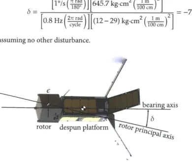
Figure 2.7: MicroMAs as a Partially-Despun Dual Spinner.
Note the smaller angular momen-tum of this system relative to the sim-ple spinner as shown in Figure 2.4.
(2.25a)
-nJPLOPL = Jy( + JPL2PL6 ) (2.25b)
-nJPL 0 PL = Jx6p + n(J-y + Jz)6p + n2(-j, + j 64 -_)JPLfPL0$
(2.25c)
2.4.1 Slewing via an External Torque
We can see the required precession torques on the left side of Equations 2.25.
The pitch torque from 2.25a is perturbational in nature, but the yaw torque from
2.25b is predictably constant and follows the form of the predicted precession torque from Equation 2.19.
2.4.1.1 ACTUATOR REQUIREMENTS Unlike in the case of the simple spinner,
only the payload is rotating, so we need to account for only its moment of inertia,
JPL:
T
prec = -nJPLOPL
= (1.1068 x 10⁻³ 1.71 g-m ( 1 kg [(2
T
rad)
(0.8 Hz)] = 9.513 pN.mWe know from examining the simple spinner case that we can get a maximum of 9.75 micronewton-meters of torque from the magnetorquers. However, pre-cessing spinner's angular momentum magnetically would not work in all parts of the orbit, since the geomagnetic field is not consistently that strong.
2.4.1.2 LINEAR STABILITY ANALYSIS: PRECESSION If we take the Laplace trans-form of this system, we can determine the short-term system behavior based
0
J(x 10=
Jy&y
30 DESIGN, ANALYSIS, & TESTING OF A PRECISION GNC SYSTEM FOR A DUAL-SPINNING CUBESAT
on the system poles. Wie performs a similar stability analysis for a simple LVLH-aligned spacecraft subject to gravity-gradient torque. He showed that for small
Wie, Space vehicle dy- angles, the pitch axis stability is decoupled from the roll and yaw axes;2
un-namics and control, p. 391- fortunately, with the payload momentum bias, this decoupling is no longer the
case, as the off-axis terms in Equation 2.25a show. The system is described in the Laplace domain as
[
s2+n7z~
=~
n<(2.26)Note the forcing term on the left hand side, which is the constant precession torque. We can find the poles of this system by setting the characteristic poly-nomial to zero; that is, setting the determinant of the dynamics matrix to zero
and solving for s. Doing so, we fid that
s = 0, 0, ±ni, ± n2(..+L+L.- 1 JJ0 'L (2.27)
\JxJ 2z Ix /x Iy(z
Thence we can derive necessary and sufficient conditions for balancing the
space-craft to achieve marginal stability.
We can also attempt to perform a linear stability analysis of the system as it is affected by environmental torques. At this point, we do not know much about the design and shape of the spacecraft other than its general mass char-acteristics and alignments, so attempting to quantify torques such as those due to aerodynamic drag or solar radiation pressure becomes impossible, because we do not know about solar panel alignment or antennas. However, the gravity gradient torque depends only upon the inertia characteristics of the system, so we can still see if analyzing gravity gradient torque is a useful pursuit. It is im-portant to note, though, that since the spacecraft will be in LEO, the drag torque may exceed the gravity gradient torque.
-3n2
U~
_
Jz)P
= fx + n(-J, + J, - Jz)02 + n2(Jy _ (2.28a)-nJPL0PL'I - gn2 J _ z~~5 yo1N6 + JPLfiPLO1P (2.28b)
-nJPL0PL = z~' +
fux
- J +Jz)0/
+ 2(-J L+JL)P
- JPL0PL6 0 (2.28c)
And in Laplace space:
1 s2+4n2Yz 0 n1+hs
os
crf
to aciee5agialsabl)y
DP 82 + P
~
+n2 PL '' 6O(S)-n 4 OLf P J~) L 5 +nhi L JPL2D+L: -0(+)
I IxJ t
~--Jz(2.29)
Setting the determinant of this dynamics matrix to zero and solving for s yields an insoluble mess that is not helpful for determining necessary and sufficient
conditions for spacecraft design. Since the maximum gravity gradient torques (which occur at a 45-degree dip angle) should be so much smaller than the re-quired precession torques anyway21, this omission should not be a problem. 2.4.2 Constant, Nonzero System Angular Momentum
Since we know that precessing the entirety of the system's momentum with the spacecraft's actuators is unrealistic, we can also consider keeping the system's angular momentum constant and trading it between momentum storage de-vices as the spacecraft rotates. Since we have reaction wheels, our dynamical equation of motion is (assuming a hypothetical infinite-bandwidth controller)
0
I
JXxx1[
(iZ
-iy) wy
wV TPL1[
0
1[TRWx1
I0
J(
y + UI-Jz)oxOz + 0 + JPLOPLz + TRWY +0 Jz(z
(iy
-ix)
OxWy 0 -JPLOPLay TRWZFor our triaxial reaction wheel set, we can trade the payload's angular momen-tum between the roll and yaw axis wheels and use the pitch axis wheel to keep the spacecraft aligned with the LVLH frame:
HRWx = HPL COS V - HPL HRWy - njy HRWz = -HPL Sin V 2Tmx =-3n 2(jx - Iz)/VZ - 3(1.1068 X 10⁻³ad)X (385.6 -647.0) kg.cm 2 (_ )2] = 67.9 nN-m JRW (ORWzWy - f)RWy0Z) JRW (nRW_6z - ORWz 6x) (2.30) JRW (URWyCX - ORWX y (2.31a) (2.31b) (2.31c) where for a circular orbit the spacecraft's true anomaly v = nt. Note that the x and z wheels are a quarter cycle out of phase. We can determine the reaction wheel speeds to command simply by dividing both sides by the reaction wheels' angular momentum: JPL JPL ORW P 0PL COS nt - PL JRW JRW 0 RW n JRW JPL ORW -- ( PLSsin nt JRW (2.32a) (2.32b) (2.32c)
Differentiating Equations 2.31 with respect to time nets us the required reaction wheel torques: TRW = -JPL 0 PL Sin nt TRW= 0 TRWz = JPLOPL COS ut (2.33a) (2.33b) (2.33c)
2.4.2.1 ACTUATOR REQUIREMENTS These required reaction wheel commands
32 DESIGN, ANALYSIS, & TESTING OF A PRECISION GNC SYSTEM FOR A DUAL-SPINNING CUBESAT
With a despun platform, the reaction wheel assembly does not rotate at o.8 hertz with the spacecraft body, negating the need for such a high reaction wheel torque requirement as the simple spinner case. Reaction wheel angular mo-mentum storage then becomes the limiting factor. Recalling location (c) in Fig-ure 2.5, the maximum angular momentum that the wheels would need to store would be twice the angular momentum of the rotating payload-2(8.6 mN.m.s) =
17.2 mN-m-s-which, while not an order of magnitude above the available mo-mentum storage, still exceeds the capabilities of the MAI-40oS actuators.
Figure 2.8: Reaction Wheel Required Speeds and Torques. Note the required x
reaction wheel speed crossing the maxi-mum available speed on v E (160', 200*).
104 Q 0 -1 0 50 100 150 200 250 300 350 .10-2 0.5-0 -0.5 0 50 100 150 200 True Anomaly, v (0) 250 300 350
" James R. Wertz, "Torque-Free Motion", p. 490.
2.4.2.2 LINEAR STABILITY ANALYSIS: NUTATION In the absence of external
torques, a momentum-biased system is subject to nutation should the axis of rotation become misaligned with a principal axis of the spacecraft.2 2
With the sinusoidal description of reaction wheel angular momentum, we cannot perform a linear stability analysis applicable to all points in the orbit; thus we will examine each quarter of the orbit, i.e., the four points from
Fig-ure 2.5. We can substitute Equations 2.17, 2.18, 2.32 and 2.33 into Equation 2.30
to obtain kinematic equations of motion for each of the four points in the orbit under review:
Point (a) 0 = Jxbk + n(-Jx - Jz)6 - n2Jz6 0 = Jyb6 + JPLOPL(n6 4P + 60) 0 = Jzb + n(fx + Jz)6b - n2Jxbp - JPL0PL66 Point (b) 0 = Jxby + n(-Jx - Jz)bp - n2jz6 - JPLfPL66 0 = Jy 6 + JPLOPL(-n6VY + 6) 0 = Jzb + nfux + Jz)b - n2 J,61p Point (c) 0 = fXby + n(-Jx - Jz)6i - n2 Jz6b
o
= jy60 + JPLOPL(-En6P - 6p)o
= Jz6p + n(Jx + Jz)64 - n2Jx61p + JPL0 PL6 0 Point (d)o
Jx6P + x(-Jx - Jz)6i - +2jzbN + JPLDPL6Oo
= Jy50 + JPL0PL(l5' - 6p) 0 = Jzb6 + n(jx + Jz)6( - n2 Jxo6pAnd in the Laplace domain:
0 0 0 0 0 0
=I
=I
s2-n 2L Ix n !hPL I n x+zs s2 -n2z I., L1-LOIPLS yn Jxi L s
Point (a) 0 S 2 -IgDOPLS Point (b) _IL OPLS 2 0 n _ _ s fi _Jx2J I S 2 - 2kx 1Z]
n -1ZS Ix -nlPL OPL s2 _ n2Ix Jz 60(s) 60(s) 01P(S) 60(s) 60b(s)I
I
0 0 0I
And setting the characteristic polynomial to zero and solving for nutational poles of the system at Points (a)-(d):
Points (a) & (c):
Points (b) & (d):
I
0 0 0 JPL s =0, 0, ±ni, J PLL_ 2 s=0, 0, ±ni, * PL - n2 JzJyI
s gives us theNote the switch of the roll and yaw inertiae in the denominators of the last poles between quadrants.
An option not examined would be to counter some portion of the angular momentum produced by the rotating payload and precess the rest with mag-netic torque. However, the angular momentum estimator required for such a solution levies additional requirements on computing resources atop those already required for attitude estimation. This solution may be useful if a zero-momentum system proves untenable.
s2-n2 Jz Ix -nJP-LOPL Iz Point (c) 0 S2 !h OPLS Point (d) /L f)PLS 2 0 Ix _IP OPLS Jy g2 - 2Ix S n SZ nJP PL s2 _ n2 L Iz