READ THESE TERMS AND CONDITIONS CAREFULLY BEFORE USING THIS WEBSITE. https://nrc-publications.canada.ca/eng/copyright
Vous avez des questions? Nous pouvons vous aider. Pour communiquer directement avec un auteur, consultez la première page de la revue dans laquelle son article a été publié afin de trouver ses coordonnées. Si vous n’arrivez pas à les repérer, communiquez avec nous à [email protected].
Questions? Contact the NRC Publications Archive team at
[email protected]. If you wish to email the authors directly, please see the first page of the publication for their contact information.
NRC Publications Archive
Archives des publications du CNRC
This publication could be one of several versions: author’s original, accepted manuscript or the publisher’s version. / La version de cette publication peut être l’une des suivantes : la version prépublication de l’auteur, la version acceptée du manuscrit ou la version de l’éditeur.
Access and use of this website and the material on it are subject to the Terms and Conditions set forth at
Lightswitch: A stochastic model for predicting office lighting energy
consumption
Newsham, G. R.; Mahdavi, A.; Beausoleil-Morrison, I.
https://publications-cnrc.canada.ca/fra/droits
L’accès à ce site Web et l’utilisation de son contenu sont assujettis aux conditions présentées dans le site LISEZ CES CONDITIONS ATTENTIVEMENT AVANT D’UTILISER CE SITE WEB.
NRC Publications Record / Notice d'Archives des publications de CNRC:
https://nrc-publications.canada.ca/eng/view/object/?id=c02ae826-1159-4f06-b3a7-9da77bb2ec78 https://publications-cnrc.canada.ca/fra/voir/objet/?id=c02ae826-1159-4f06-b3a7-9da77bb2ec78
Lightswitch: A stochastic model
for predicting office lighting
energy consumption
Newsham, G.R.; Mahdavi, A.; Beausoleil-Morrison, I.
NRCC-38939
A version of this document is published in / Une version de ce document se trouve dans:
Right Light Three : 3rd European Conference on Energy- Efficient Lighting, Newcastle, U.K. June
18-21, 1995, pp. 59-66
The material in this document is covered by the provisions of the Copyright Act, by Canadian laws, policies, regulations and international agreements. Such provisions serve to identify the information source and, in specific instances, to prohibit reproduction of materials without written permission. For more information visit http://laws.justice.gc.ca/en/showtdm/cs/C-42
Les renseignements dans ce document sont protégés par la Loi sur le droit d’auteur, par les lois, les politiques et les règlements du Canada et des accords internationaux. Ces dispositions permettent d’identifier la source de l’information et, dans certains cas, d’interdire la copie de documents sans permission écrite. Pour obtenir de plus amples renseignements : http://lois.justice.gc.ca/fr/showtdm/cs/C-42
3rd European Conference on Energy-Efficient Lighting
LIGHTING SYSTEMS AND APPLICATIONS
GUY NEWSHAM
M-24, National Research Council Canada, Montreal Rd, Ottawa, Ontario, CANADA, K1A OR6. ARDESHIR MAHDAVI
CBPD, Dept of Architecture, Carnegie Mellon University, Pittsburgh, PA 15213-3890, USA. IAN BEAUSOLEIL-MORRISON
CANMET, Natural Resources Canada, 580 Booth St, Ottawa, Ontario, CANADA, K1A OE4.
LIGHTSWITCH: A STOCHASTIC MODEL FOR PREDICTING
OFFICE LIGHTING ENERGY CONSUMPTION
ABSTRACT
Lighting controls are promoted on the basis that they significantly reduce lighting energy consumption. We are currently studying the impact of lighting controls on office building energy consumption using the DOE2.1 E building energy model. In DOE2.1 E the lighting load is defined by an hourly profile. Modelling lighting controls (other than daylighting, which can be modelled dynamically) is achieved by inputting different profiles. However, representative profiles, particularly those showing the impact of lighting controls, are not readily available. Consequently, we decided to develop a model (LIGHTSWITCH) to predict lighting profiles for a typical office.
For example, the impact of occupancy sensors clearly depends on the building occupancy: arrival times, departure times, and times of temporary absence. There is randomness to these occupancy parameters, therefore LIGHTSWITCH is a stochastic model which incorporates randomness based on observed occupancy behaviour. LIGHTSWITCH can model the impact of occupancy sensors of variable switching delays, daylighting controls, and zoning.
INTRODUCTION
There are many energy efficient lighting and office equipment technologies available for application in office buildings {IRC 1994, Webster 1994, Lovins and Heede 1990, BRE 1983, Richardson Assoc. Ltd. 1990). The number of such products, and the interest in installing them, is increasing, driven by the support of utilities and codes (ASHRAEIIES 1989). The claimed efficiency of these products, which is often impressive, is almost always based on "performance in isolation•. The actual net benefit from these products may vary from the quoted performance for a number of reasons. These reasons include control and operation of the products and, the interaction of the products with other building systems. For example, a more efficient product generates less heat than the product it replaces. In a heating climate, this difference in heat must be provided by another heat source. Thus, the net energy benefit of adopting the product will be reduced. Conversely, in a cooling climate, the net energy benefit of adopting the product will be amplified by a reduced building cooling load. Most office buildings in North America experience both heating and cooling climates during a year.
NORTHERN ELECTRIC
セ@
..
Peak loads and energy consumption can be reduced further by controls which ensure the use of electrical products is more closely related to demand. Examples of control technologies for lighting systems are occupa11cy sensors and daylight linked dimming systems.
Zoning of building systems can also have a significant effect on overall energy consumption. For example, small zones will clearly enhance the benefits of occupancy sensor controlled lighting; a smaller zone (for example, a single workstation) is vacated more frequently than a larger zone. Similar benefits could be realized by HVAC (heating, ventilating and air-conditioning) zoning (Mahdavi et al. 1994).
Only detailed modelling, which simulates the interactions between various building systems, can properly resolve the net benefit of the adoption of energy efficient products, control strategies, and zoning strategies. We are currently studying the impact of energy efficient products, control strategies, and zoning strategies on office building energy consumption using the DOE2.1 E building energy model (Winkelmann et al. 1993). We are focusing on the following technologies:
• energy efficient light fixtures; • lighting controls;
• l<;>w power office equipment;
• power management of office equipment.
In this paper we will concentrate on how we model the impact of lighting controls using DOE2.1 E, particularly how we model the impact of occupancy sensors.
In DOE2.1 E the lighting load is defined by an hourly utilization profile. Daylighting strategies can be modelled dynamically, and modelling of other controls, including occupancy sensors, is achieved by inputting different utilization profiles. Therefore, when modelling the impact of occupancy sensors, two utilization profiles are needed:
(1) a base lighting utilization profile prior to the adoption of occupancy sensors; (2) a lighting utilization profile after the adoption of occupancy sensors.
Well documented studies showing ubefore and after" lighting utilization profiles from buildings that have undergone occupancy sensor retrofit are not readily available. Even those studies which are available (Turner 1982, Crosbie 1993) provide information specific to the building in which the measurements were made. The results cannot necessarily be generalized and applied to buildings with, for example, different occupancy schedules and different sensor characteristics. Consequently, we decided to develop a model (LIGHTSWITCH) to predict lighting utilization profiles for a typical office.
CALCULATING OCCUPANCY
In office buildings where the lighting is switched predominantly by the building occupants, the lighting utilization profile clearly depends on the building occupancy: arrival times, departure times, and times of temporary absence. Therefore, to model lighting utilization we must first model occupancy. In a real office building, there is some randomness to occupancy parameters. For example, though work may officially begin at 8:30am, not everyone will arrive at exactly 8:30 am. Some people will be early, some late, some will be delayed by work commitments outside the office, some will be away for the day. This behaviour will not be the same from day to day in a particular building, nor will the behaviour be the same from building to building. To accommodate this type of behaviour in a model of lighting utilization we require the model to be stochastic (to incorporate randomness), and based on observed occupancy behaviour.
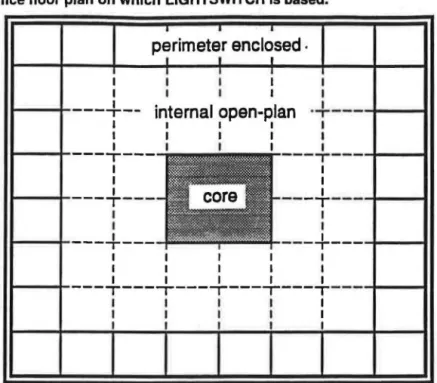
The current version of LIGHTSWITCH is based on a single office floor, shown in Figure1. The floor plan is divided into 64 regions of equal area. The centre 4 regions represent the core zone. Lighting in the core zone is generally isolated from the lighting in the rest of the floor and is thus ignored by LIGHTSWITCH. The remaining 60 regions are assumed to be offices associated with a single occupant. The offices are assumed to be of equal area, which might be 6 to 8 m2 in a typical office. There are 28 enclosed offices on the perimeter, and 32 open-plan offices toward the centre of th.e floor open-plan; circulation space is not treated separately.
Figure 1. Office floor plan on which LIGHTSWITCH is based.
perimeter enclosed .
I I I I I I I I1--r---+--
internal open-plan
·+----t---t
I I I I I I I I I I I I I I It---+----,----
---,---t----1
I I I I I It---+----T---
-T----1---t
I I I I1----t----+--
KMMMMKMMセQQ@ I I I I I I I I I1---t----,----.---.----,----,---+----1
I I I I I I I I I I I I I I IWhether a zone is occupied or vacant depends on the outcome of three stochastic routines: the first determines if the occupant has arrived at work; the second determines if the occupant is temporarily away from his/her desk; and the third determines if the occupant has departed for the day.
For modelling purposes the day is divided into discrete 5 minute intervals (or timesteps). Each one of the routines is evaluated for every occupant, every timestep. Each time an evaluation is made a random number is generated. This random number is compared to a specified probability to determine an outcome. For example, a routine might state:
IF THE TIME IS 9 AM AND THE RANDOM NUMBER IS LESS THAN 0.1, THEN THE OCCUPANT HAS ARRIVED.
In most office buildings the probability of an occupant arriving at 9 am is greater than the occupant's probability of departing at 9 am. The probability of arrival will usually build to a peak at a certain time and then decrease again. Therefore we expect that the probability associated with each routine will vary with time.
We used observed data to determine arrival, temporary absence, and departure probabilities which, when incorporated into LIGHTSWITCH, yielded occupancy profiles similar to those observed. We extrapolated arrival probabilities from the recorded computer network logon times of 240 employees at one site over 1 B days. We derived temporary absence probabilities from walk-throughs at a second site with around 80 employees. Each employee's presence or absence was noted twice per day for 12 days; the walk-throughs occurred at different times each day. We did not observe departure behaviour in real buildings. Rather, we chose departure probabilities that produced behaviour typical of real buildings.
Figure 2 shows the variation of probability with time for each routine. There are two sets of probabilities associated with temporary absence. If the occupant is at his/her desk the probability of him/her leaving in the timestep is typically 0. 12. However, if the occupant is already absent, the probability of him/her continuing to be absent is typically 0.60. Observe the increase in probability of temporary absence around lunchtime.
Note that the arrival, temporary absence, and departure routines presented in this paper are based on preliminary data, and serve to generate profiles for the DOE 2.1 E modelling described in the Introduction. The same routines may not be appropriate for all buildings. Observation of occupancy behaviour may be necessary to generate appropriate routines for other building types.
CALCULATING LIGHTING UTILIZATION
Once the occupancy is det_ermined, we are in a position to derive the lighting utilization. At present, we make the assumption that the maximum lighting power associated with each office is the same. At this stage we are not concerned with the actual lighting power in each office, only the fraction of offices where the electric lighting is utilized. Initially, the lighting in an office is considered to be switched on when the occupant arrives, and switched off when the occupant leaves. However, this can be modified by the lighting option or options specified. The following options are available, and can be modelled separately, or in combination:
Figure 2. Probability vs. time for the arrival, departure, and temporary absence routines.
0.1 iii 0.08
セ@
Ill 0 0.06A
セ@:E
0.04 Ill ..Qe
Q.0.02 0 0 2 4 6 8 10 12 14 16 18 20 22 24 tlme, h 0.6 ! 0.5 セ@ Ill Q.0.4-!
00.3 セ@:c
0.2 Illセ@
Q.0.1 0 セ@ 0 2 4 6 8 10 12 14 16 18 20 22 24 time, h セ@1r---.
i
.g
0.8!
0 0.6 セ@ Gl=
0.4 0 セ@:E
0.2. .
.
.
i!madyab5CIII if c:um:ndy at do:sk セ@ r - - - ' c. 0 MQMMMMMMMMMMMMMMMMMセMMMNNMMNNNNNMMMェ@ 0 2 4 6 8 10 12 14 18 18 20 22 24 tlme,hPerimeter-Internal Zoning: If this option is chosen, all the lighting associated with the internal,
open plan offices is switched on whenever at least one of the internal offices is occupied.
Occupancy Sensors: If this option is chosen then the lighting of each office is switched off if the
occupant is temporarily away from the office for more than a specified number of timesteps; the lighting is switched back on キィセョ@ the occupant returns. Note that if the perimeter-internal zoning option is also chosen, only the perimeter offices will benefit from occupant sensors.
Perimeter Daylight: If the calculated daylight illuminance in the perimeter offices is greater than
a specified level then the lighting in the office is dimmed by a specified amount. At present the daylight is simply calculated using a daylight factor (Hopkinson et al. 1966) input by the user, and nominal external daylight data.
Internal Daylight: If the calculated daylight illuminance in the internal offices is greater than a
specified level then the lighting in the office is dimmed by a specified amount. At present the daylight is simply calculated using a daylight factor (Hopkinson et al. 1966) input by the user, and nominal external daylight data.
GRAPHIC PRESENTATION
Figure 3 shows an example LIGHTSWITCH output screen; in this case there is perimeter-internal zoning, but no occupancy sensors or daylight dimming. The time in the upper right indicates that this screen is a snapshot taken at the timestep representing 2:25 pm. On the left of Figure 3 is the floor plan divided into the 64 regions. The white squares indicate offices where the lighting is switched off; note, this includes the central 4 regions which form the core. The shaded squares indicate offices where the lighting is switched on. The circles indicate offices which are currently occupied. Offices in which lighting is on but that are unoccupied are the result of the occupant being temporarily absent from his/her desk. Note that the lighting is on in all 32 internal offices, due to the perimeter-internal zoning option.
Figure 3. The LIGHTSWITCH output screen.
t
h••·
1"'1:25 80 :JIS"'' u c"
-48!
H
32 0 16 sa 24 hour 80 6"'1•
..
i
"'18r-..
...
32 1S 2"1 hourOn the right of the display are two graphs. The upper graph indicates the occupancy profile. The upper of the two curves shows the number of occupants who have arrived for work (and who have not yet departed). The lower of the two curves shows the number of occupants who are at their desk; note the dip in occupancy (increase in temporary absence) at lunchtime.
The lower graph indicates the lighting profile. The curve indicates the number of offices in which the lighting is on.
NEWSHAM, MAHDAVI, BEAUSOLEIL-MORRISON 63
..
!'
t
i
APPLYING LIGHTSWITCH
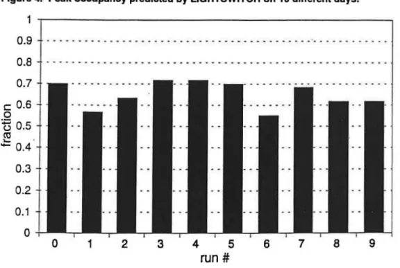
The first application of LIGHTSWITCH was to generate a base lighting profile for the DOE2.1 E modelling described in the Introduction. For the base case, we assumed perimeter-internal zoning, but no occupancy or daylighting controls. Fig.ure 4. shows the peak occupancy predicted by the model on 1 0 different days.
Figure 4. Peak occupancy predicted by LIGHTSWITCH on 10 different days.
0.9 ... .. ... . ... "' ... - ... - ... - - ... . ... · ... - . 0.8 .. ... - ... "' ... "' ... - ... - - .. ... ... ... - .. .. ... ... .
0.7
c
0.6
0t5
0.5
セ@-
0.4
0.3
0.2
0.1
0
0
1
2
3
4
5
6
7
8
9
run#
Due to the stochastic nature of the model, the peak occupancy varies from day to day, just as it does in a
real building. Therefore, we decided to take the average profiles from the 10 runs as the input to DOE2. 1 E. These average profiles are shown in Figure 5.
Figure 5. Average occupancy and lighting profiles predicted by LIGHTSWITCH.
0.9 0.8 0.7 c:: 0.6 0
u
0.5 ctl ... -0.4 0.3 0.2 0.1 0 64 0· · · ·Ifghtiiti · · · • · · ·
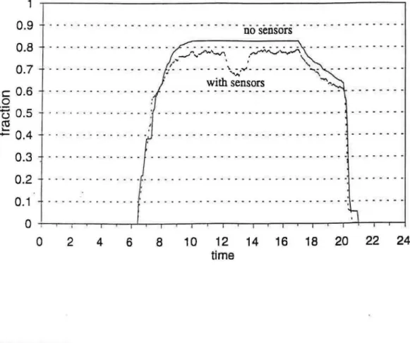
· · · · · · · · · · · · · · · arrived at work · · · -2 4 6 8 10 12 14 16 18 20 22 24 timeWe then generated a lighting profile in the case where occupancy sensors were assumed for the perimeter offices. The lighting in the office was switched off after 2 consecutive timesteps (10 minutes) of temporary absence, and switched on again as soon as the occupant returned. Again, the average over 10 runs was calculated. Figure· 6 compares the profile generated assuming occupancy sensors for the perimeter offices with the profile assuming no occupancy sensors. Occupancy sensors do lower the lighting utilization profile, particularly at lunchtime. Note that to generate a total lighting utilization profile we will include an additional utilization fraction (5 % or less), constant for all hours, to account for emergency and core lighting.
Figure 6. Lighting profiles predicted by LIGHTSWITCH; profiles assuming no occupancy sensors and assuming occupancy sensors in the perimeter offices are shown .
1
0.9
0.8
0.7
c
0.6
0u
0.5
co
.:: 0.4
0.3
0.2
no sensors
• a • 4 4 4 4 • w , . • ,. , . • ,. • , . • ,. ⦅[ヲ|セセ [N LZ⦅[⦅@• ., •
LZLN[M[セセ@ 4 • . , , . • • • • • A • • • •ゥGセ@
- 4 '... . ...
·
... ...
;..•"'
...
"""
... .
· withsensors
GBBセ@ .. .. セ@-
.-
.-
- ..
.. ..
.
. ..
.. - .-
..-
. . .
..
.. .. .. . .. .. ... . .
.. ...
"' ..-
...
.-
...
.. .. ..0.1
.. - .. .. .. . .. .. .. .. .. . . .... - . - - ... - ... - - - .... - ... - - ... - - "'
0
K N セセセセセセセセセセセセセセセセセセセセMMセセ@0
2
4
68
1 0
12
14
16
18
20
22
24
time
CONCLUSIONSLIGHTSWITCH successfully uses observed occupancy data to produce realistic occupancy and lighting profiles. Constructing the lighting utilization profiles from occupancy profiles allows the performance of occupancy sensors to be modelled accurately. Due to the stochastic nature of the model, the profiles predicted are different from day to day; this variation is similar to that observed in real buildings.
The occupancy data on which LIGHTSWITCH is based were derived from a limited dataset. More data collection is required to develop more truly representative lighting profiles.
In the present application, we use multiple runs to produce an average lighting utilization profile which is then fixed and applied to all days. In the future, it may be possible to incorporate LIGHTSWITCH into a larger stochastic building energy model that could use a different lighting utilization profile for each modelled day. Thus, the stochastic-, occupancy-based, approach adopted by LIGHTSWITCH holds the promise of more realistic and accurate modelling of occupied buildings in the future.
REFERENCES
ASHRAE/IES. 1989. Energy efficient design of new buildings except new /ow-rise residential buildings. ASHRAE Standard 90. 1. American Society of Heating, Refrigerating and
Air-conditioning Engineers, Atlanta, USA.
BRE. 1983. Lighting Controls and Daylight Use . BRE Digest No. 272. Building Research
Establishment, Garston, UK.
Crosbie, M. J. 1993. "Practicing what they Preach." Progressive Architecture, (3):84-89.
Hopkinson, R. G., P. Petherbridge,
J.
Longmore. 1966. Daylighting. Heinemann, London, UK.IES. 1993. Lighting handbook. Illuminating Engineering Society of North America, New York,
USA.
IRC. 1994. Effective and efficient lighting. Building Science Insight '92. National Research
Council of Canada, Ottawa, Canada.
Lovins, A. B., and H. R. Heede. 1990. Electricity-Saving Office Equipment. Competitek, Rocky
Mountain Institute, Boulder, USA.
Mahdavi, A., P. Mathew, S. Kumar, V. Hartkopf, and V. Loftness. 1994. "Effects of Lighting, Zoning and Control Strategies on Energy Use in Commercial Buildings." Proceedings of the
1994 IESNA Annual Conference. Illuminating Engineering Society of North America, New York, USA.
Richardson & Associates Ltd. 1990. Flexibility and Economics of Lighting Controls. CEA
Report No. 722 U 705. Canadian Electrical Association, Montreal, Canada.
Turner, 0. 1982. Occupancy Controlled Lighting: Energy savings Demonstration and Analysis.
ERDA Report No. 82-33. New York State Energy Research and Development Authority, Albany, USA.
Webster, L. 1994. Retrofitting Computers and Peripherals for Energy Efficiency. Tech Update
TU-94-8. E SOURCE, Boulder, USA. .
Winkelmann, F. C., B. E. Birdsall, W. F. Buhl, K. Ellington, A. E. Erden, J. J. Hirsch, S. Gates. 1993. DOE-2 Supplement Version 1.1E. Lawrence Berkeley Laboratory, Berkeley, USA.