Dynamically Orthogonal Numerical Schemes for
Efficient Stochastic Advection and Lagrangian Transport
The MIT Faculty has made this article openly available.
Please share
how this access benefits you. Your story matters.
Citation
Feppon, Florian, and Pierre F. J. Lermusiaux. “Dynamically
Orthogonal Numerical Schemes for Efficient Stochastic Advection
and Lagrangian Transport.” SIAM Review 60, no. 3 (January 2018):
595–625. © 2018 Society for Industrial and Applied Mathematics.
As Published
http://dx.doi.org/10.1137/16M1109394
Publisher
Society for Industrial and Applied Mathematics
Version
Final published version
Citable link
http://hdl.handle.net/1721.1/119800
Terms of Use
Article is made available in accordance with the publisher's
policy and may be subject to US copyright law. Please refer to the
publisher's site for terms of use.
Dynamically Orthogonal Numerical
Schemes for Efficient Stochastic Advection
and Lagrangian Transport
\ast
Florian Feppon\dagger Pierre F. J. Lermusiaux\dagger
Abstract. Quantifying the uncertainty of Lagrangian motion can be performed by solving a large num-ber of ordinary differential equations with random velocities or, equivalently, a stochastic transport partial differential equation (PDE) for the ensemble of flow-maps. The dynam-ically orthogonal (DO) decomposition is applied as an efficient dynamical model order reduction to solve for such stochastic advection and Lagrangian transport. Its interpre-tation as the method that applies the truncated SVD instantaneously on the matrix dis-cretization of the original stochastic PDE is used to obtain new numerical schemes. Fully linear, explicit central advection schemes stabilized with numerical filters are selected to ensure efficiency, accuracy, stability, and direct consistency between the original determin-istic and stochastic DO advections and flow-maps. Various strategies are presented for selecting a time-stepping that accounts for the curvature of the fixed-rank manifold and the error related to closely singular coefficient matrices. Efficient schemes are developed to dynamically evolve the rank of the reduced solution and to ensure the orthogonality of the basis matrix while preserving its smooth evolution over time. Finally, the new schemes are applied to quantify the uncertain Lagrangian motions of a 2D double-gyre flow with random frequency and of a stochastic flow past a cylinder.
Key words. dynamically orthogonal decomposition, stochastic advection, singular value decomposi-tion, uncertainty quantificadecomposi-tion, flow-map, Lagrangian coherent structures
AMS subject classifications. 65C20, 53B21, 15A23, 35R60 DOI. 10.1137/16M1109394
Contents
1 Introduction 596
2 Dynamically Orthogonal Stochastic Transport Equations 600
2.1 Mathematical Setting for the Transport PDE . . . 600
2.2 The DO Field Equations . . . 601
2.3 Geometric Framework in Matrix Spaces and Theoretical Guarantees . 602
3 Implementation of the DO Approximation for Stochastic Advection 604
\ast Received by the editors December 27, 2016; accepted for publication (in revised form) August
23, 2017; published electronically August 8, 2018.
http://www.siam.org/journals/sirev/60-3/M110939.html
Funding: This work was supported by the Office of Naval Research under grants N00014-14-1-0725 (Bays-DA) and N00014-14-1-0476 (Science of Autonomy -- LEARNS) and by the National Science Foundation under grant EAR-1520825 (Hazards SEES -- ALPHA), each to the Massachusetts Institute of Technology.
\dagger MSEAS, Massachusetts Institute of Technology, Cambridge, MA 02139 ([email protected],
3.1 Motivations for Linear Advection Schemes . . . 604
3.2 Boundary Conditions . . . 606
3.3 Low-Rank Time-Stepping . . . 608
3.4 Dynamically Increasing the Rank of the Approximation . . . 611
3.5 Preserving the Orthonormality of the Mode Matrix U . . . 612
4 Numerical Results 614 4.1 Stochastic Double-Gyre Flow . . . 614
4.2 Stochastic Flow Past a Cylinder . . . 617
5 Conclusion 620
References 622
1. Introduction. Advection plays a major role in a wide variety of physical
pro-cesses and engineering applications of fluid mechanics [26, 3], neutronic transport, chemical transports, atmospheric sciences [62], and ocean sciences [20, 53]. At its most fundamental level, the pure advection process is commonly understood through the transport partial differential equation (PDE),
(1)
\Biggl\{
(\partial t+ \bfitv (t, \bfitx ) \cdot \nabla )\bfitpsi = 0,
\bfitpsi (0, \bfitx ) = \bfitpsi 0(\bfitx ),
which models the material transport of a passive (scalar or vectorial) tracer field \bfitpsi
under a velocity field \bfitv , having its values initially distributed as \bfitpsi 0 over a physical
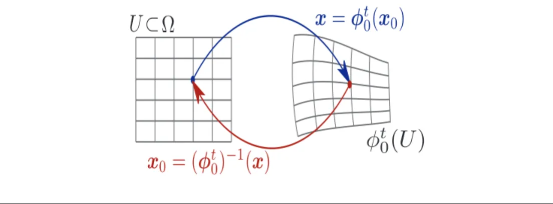
domain \Omega \subset \BbbR d of positions \bfitx . Another description of transport considers a parcel of
material initially located at the location \bfitx 0and transported to the position \bfitphi t0(\bfitx 0) =
\bfitx (t) with instantaneous velocity \bfitv (t, \bfitx (t)). In this Lagrangian description, \bfitx (t) is the solution of the ordinary differential equation (ODE)
(2)
\Biggl\{ \.
\bfitx =\bfitv (t, \bfitx (t)), \bfitx (0) =\bfitx 0,
and \bfitphi t
0, i.e., the function mapping the initial positions \bfitx 0to \bfitphi t0(\bfitx 0) = \bfitx (t) at time t,
is the flow-map of the ODE (2). Under sufficient regularity conditions on the velocity field \bfitv [9, 2], the solution \bfitpsi of the advection equation (1) relates to equation (2) as being obtained by ``carrying \bfitpsi 0 values along the particles' paths"":
(3) \bfitpsi (t, \bfitx ) = \bfitpsi 0((\bfitphi t0) - 1(\bfitx )),
where (\bfitphi t
0) - 1is the backward or inverse flow-map (Figure 1). In fact, (1) and (2) are
equivalent mathematical descriptions of material transport, as setting \bfitpsi 0(\bfitx ) = \bfitx in
(3) yields \bfitpsi (t, \bfitx ) = (\bfitphi t
0) - 1(\bfitx ). Similarly, solving the transport equation backward in
time with the terminal condition \bfitrho t(\bfitx ),
(4)
\Biggl\{
(\partial s+ \bfitv (s, \bfitx ) \cdot \nabla )\bfitrho = 0,
\bfitrho (t, \bfitx ) = \bfitrho t(\bfitx ),
allows us to retrieve the forward flow-map from the relation \bfitrho (s, \bfitx ) = \bfitrho t(\bfitphi t s(\bfitx ))
by setting \bfitrho t(\bfitx ) = \bfitx . This shows that the flow-map \bfitphi t
0 can be obtained from a
Fig. 1 Illustration of the action of the forward and backward flow-map on a subdomain U \subset \Omega of a spatial domain \Omega \subset \BbbR d. \bfitphi t
0 maps initial particle positions \bfitx 0 to their position at time t,
and (\bfitphi t
0) - 1 is the reciprocal map.
solution of the transport PDE (1), and vice versa. This property has been thoroughly investigated on the theoretical side to provide a mathematical meaning to the solutions of the ODE (2) for velocity fields \bfitv with weak regularity [9, 2, 4], and more recently in numerical computations, as it offers an alternative method to direct particle advection
for the evaluation of the flow-map \bfitphi t0 [44, 45].
A typical challenge encountered in environmental flow predictions is the need to deal with velocity data that include a certain level of uncertainty, resulting from sparse data acquisitions, noise in direct measurements, or errors in the inferred numerical predictions [41]. Uncertainty is modeled by including randomness in the velocity field [39]: each realization, \bfitv (t, \bfitx ; \omega ), corresponds to a particular possible scenario, \omega . An issue of great interest in hazard predictions [33] is to quantify how this uncertainty reverberates in the Lagrangian motion [42]. A basic Monte Carlo (MC) approach would then solve either the stochastic ODE
(5)
\Biggl\{ \.
\bfitx = \bfitv (t, \bfitx ; \omega ), \bfitx (0) = \bfitx 0,
or the stochastic PDE (SPDE)
(6)
\Biggl\{
\partial t\bfitpsi + \bfitv (t, \bfitx ; \omega ) \cdot \nabla \bfitpsi = 0,
\bfitpsi (0, \bfitx ) = \bfitx ,
for a large number of realizations, \omega . While performance of particle as well as MC methods can be optimized through parallelism, such methodologies are computation-ally demanding for cases requiring high resolution in both the spatial and stochastic domains, i.e., large numbers of particles and realizations. Hence, while they have been useful in a variety of applications [6, 46], particle and MC methods are very expensive for uncertain advection.
A substantial benefit of the PDE formulation (6) is its compatibility with dy-namical model order reduction, which takes direct advantage of the spatial structures
in the solution. Classic reduced-order methods aim to evolve low-rank
decompo-sitions such as \bfitpsi (t, \bfitx ; \omega ) \simeq \sum r\Psi
i=1\zeta i(t; \omega )\bfitu i(\bfitx ) or \bfitpsi (t, \bfitx ; \omega ) \simeq \sum r\Psi
i=1\zeta i(\omega )\bfitu i(t, \bfitx ),
at a cost much smaller than the direct realization methods [75, 19], by
indepen-dently evolving a small number r\Psi of spatial modes, \bfitu i, or stochastic coefficients,
\zeta i. For model order reduction of SPDEs, classic methods such as polynomial chaos
[56, 28, 84, 13], proper orthogonal decomposition (POD) [26, 60], dynamic mode de-composition (DMD) [61, 66, 78, 82, 31], and stochastic Galerkin schemes and adjoint
methods [10, 7] assume a priori choices of time-independent modes \bfitu i(\bfitx ) and/or rely
on Gaussianity assumptions on the probability distribution of the coefficients \zeta i. For
example, the popular data POD [26] and DMD [66] methods suggest extracting
time-independent modes \bfitu i(\bfitx ) that respectively best represent the variability (for the POD
method) or the approximate linear dynamics (for the DMD method) of a series of snap-shots \bfitu (tk, \bfitx , \omega 0) for a given observed or simulated realization \omega 0. These modes allow
us to quickly obtain information about the dynamics of this time series and then to
in-fer simple reduced-order models for evolving the coefficients \zeta i(t; \omega ) of a more general
solution \bfitu (t, \bfitx ; \omega ) by Galerkin projection. DMD and POD may be very useful and
efficient methods to analyze the given time series \bfitu (tk, \bfitx ; \omega 0) and infer information
about its hidden dynamics, but the use of the inferred reduced-order model may be allowed only if the variability of the observed snapshot is sufficiently representative, in both time and stochastic domains, of the nonreduced stochastic solution \bfitu (t, \bfitx ; \omega ). As will be demonstrated hereafter, the dynamically orthogonal (DO) equations overcome this difficulty as they allow us to predict both the variability and the time evolution of the stochastic solution \bfitu (t, \bfitx ; \omega ) solely from its nonreduced dynamics.
In general, the above methods may not be well suited for capturing low-rank solutions that do not decompose on a small number of time-invariant modes (e.g., as in POD and DMD), or that exhibit spatial irregularities not easily captured by Fourier modes (e.g., as in spectral methods), or for multimodal and non-Gaussian behaviors of the coefficients (e.g., as in polynomial chaos methods). This is especially the case with material transport, as advection tends to create fine features in the solution, with sharp gradients or shocks that evolve in time and space. Capturing them requires careful numerical schemes [55, 54, 71, 48]. Upwinding, total variation diminishing (TVD), and essentially nonoscillatory (ENO) schemes use diverse rules depending on the sign of the advecting velocity. How to adapt these schemes for reduced-order numerical advection, which cannot afford examining the realizations individually, is therefore particularly challenging [77, 80, 65]. This explains in part why many stochastic advection attempts have essentially restricted themselves to 1D applications [19, 28, 13, 56] or simplified 2D cases that do not exhibit strong shocks [81].
In contrast with these reduced-order methods, the DO methodology [63, 64] solves dynamical equations to simultaneously evolve a time-dependent basis of modes, \bfitu i(t, \bfitx ), and coefficients, \zeta i(t; \omega ):
(7) \bfitpsi (t, \bfitx ; \omega ) \simeq
r\Psi
\sum
i=1
\zeta i(t; \omega )\bfitu i(t, \bfitx ) .
This dynamic approach [37] can efficiently capture the evolving spatial flow features and their variability at the minimal condition that such a modal approximation (7) exists for the nonreduced solution \bfitpsi (t, \bfitx ; \omega ) [30, 52, 17]. Numerical schemes for DO equations were derived for a variety of dynamics, from stochastic Navier--Stokes [80] to Hamilton--Jacobi [74] equations. Recently, using differential geometry, the DO equa-tions were shown [17] to be instantaneously optimal among any other reduced-order model. In fact, a nonintrusive matrix version of the DO approach was independently
introduced to efficiently evolve time-dependent matrices [30]. Dynamical systems
that continuously perform classic matrix operations [5, 8, 73, 12] or learn dominant Kalman filter subspaces [34, 36] have also been derived. However, critical research
questions remain for stochastic DO transports. They relate to the consistency of the direct MC integration with the numerical DO integration, to the ill-conditioning of the coefficient matrix [49] (related to the curvature of the reduced-rank manifold), to the need to capture the sharp local gradients of the advected fields, and to the issue of maintaining the numerical orthonormality of the dynamic modes.
The purpose of this article is thus to utilize the DO decomposition [63] and its geometric interpretations [17] to obtain a systematic, optimal reduced-order method for equation (6) and to derive new numerical schemes that answer the above questions for stochastic advection and Lagrangian transports. For the latter, as an immediate benefit, a novel and efficient computational methodology for evaluating an ensemble of flow-maps \bfitpsi (t, \bfitx ; \omega ) = \bfitphi t
0(\bfitx ; \omega ) of the ODE (5) with random velocity is obtained.
The issue of shock capturing is addressed by considering fully linear but stabilized advection schemes. This provides deterministic-stochastic consistency and compatible reduced-order schemes that rely on tensor decompositions of either the solution, \bfitpsi , or its time derivative, - \bfitv \cdot \nabla \bfitpsi . The schemes obtained are not restricted to pure transport; they are also applicable to SPDEs with advection terms of the form \bfitv \cdot \nabla , such as the Navier--Stokes equations.
A synopsis of the coupled DO PDEs for the dynamical evolution of the tensor decomposition (7) is given in section 2. Numerical schemes for this set of PDEs are obtained by applying the DO methodology directly to the spatial discretization of the stochastic transport PDE rather than its continuous version (6). In that framework, the DO equations find rigorous geometric justification, corresponding to optimality conditions [17, 30, 52]. Section 3 focuses on the implementation in practice of the DO machinery to solve the stochastic transport PDE (6). Factorization properties of the advection operator must be preserved at the discrete level to ensure deterministic-stochastic consistency and avoid additional approximations. This is ensured through the selection of a fully linear advection scheme whose accuracy and stability are ob-tained by the use of high-order spatial and temporal discretization combined with linear filtering, a technique popular in ocean modeling [68, 34]. It is explained how stochastic boundary conditions (BCs) can be accounted for by the model order re-duced method in an optimal and convenient manner. Different possible time-steppings for the DO equations are discussed, as well as the issue of modifying dynamically the
stochastic dimensionality r\Psi of the tensor approximation (7). Finally, as a
require-ment of both the DO method and multisteps time-marching schemes, an efficient
method is proposed for preserving the orthonormality of the modal basis (\bfitu i) during
the time integration, as well as the smooth evolution of this basis and the coefficients
\zeta i. Numerical results of the overall methodology are presented in section 4 using the
bidimensional stochastic analytic double-gyre flow and stochastic flow past a cylin-der, both of which include sharp gradients. The DO results are finally contrasted with those of direct MC.
Notation. Important notation is summarized below:
\Omega \subset \BbbR d Spatial domain
\bfitx \in \Omega Spatial position \bfitv (t, \bfitx ; \omega ) Stochastic velocity field \bfitpsi (t, \bfitx ; \omega ) \simeq \sum r\Psi
k=1\zeta k(t; \omega )\bfitu k(t, \bfitx ) Rank-r\Psi tensor approximation of the stochastic
solution of the transport PDE (6) \scrM l,m Space of l-by-m real matrices
\Psi i,\alpha (t) \simeq \bfitpsi (t, \bfitx i; \omega \alpha ) Full-rank discrete approximation \Psi (t) \in \scrM l,m
of the continuous solution \bfitpsi
Ui,k(t) = \bfitu k(t, \bfitx i), Z\alpha ,k(t) = \zeta k(t; \omega \alpha ) Discrete approximation of the modes and the coefficients
with U \in \scrM l,r\Psi , U
TU = I, Z \in \scrM
m,r\Psi , and rank(Z) = r\Psi
M = \{ \Psi \in \scrM l,m| rank(\Psi ) = r\Psi \} Fixed-rank matrix manifold
\Psi (t) = U (t)Z(t)T\in M Rank-r
\Psi approximation of the discretized solution \Psi (t)
\scrT (\Psi ) Tangent space at \Psi \in M \scrN (\Psi ) Normal space at \Psi \in M
\Pi \scrT (\Psi ) Orthogonal projection onto the plane \scrT (\Psi )
\Pi M Orthogonal projection ontoM or rank r\Psi --truncated SVD
I Identity mapping
AT Transpose of a square matrix A
\langle A, B\rangle = Tr(ATB) Frobenius scalar product for matrices
\langle \bfitu , \bfitv \rangle L2scalar product for functions \bfitu , \bfitv over \Omega \subset \BbbR d
| | A| | = Tr(ATA)1/2 Frobenius norm
\sigma 1(A) \geq \cdot \cdot \cdot \geq \sigma rank(A)(A) Nonzero-singular values of A \in \scrM l,m
\.
\Psi = d\Psi /dt Time derivative of a rank-r\Psi solution \Psi
\rho \Psi Retraction on the manifoldM at \Psi \in M
2. Dynamically Orthogonal Stochastic Transport Equations.
2.1. Mathematical Setting for the Transport PDE. The stochastic transport
PDE (6) is set on a smooth bounded domain \Omega of \BbbR d, where d denotes the spatial
dimension. The flow-map \bfitphi t
0 of the ODE (5) is defined for all time if particle
trajec-tories don't leave the domain \Omega , which is ensured if the normal flux \bfitv \cdot \bfitn vanishes on the boundary \partial \Omega , with \bfitn denoting the outward normal of \Omega . In the following, we deal with the more general case where \bfitv \cdot \bfitn may have an arbitrary sign on \partial \Omega . Inlet and outlet boundaries are denoted, respectively, by
\partial \Omega - (t; \omega ) = \{ x \in \partial \Omega | \bfitv (t, x; \omega ) \cdot \bfitn < 0\} ,
\partial \Omega +(t; \omega ) = \{ x \in \partial \Omega | \bfitv (t, x; \omega ) \cdot \bfitn \geq 0\} .
Boyer [4] has shown that the transport equation (6) is well posed (under suitable regularity assumptions on \bfitv ), provided a Dirichlet BC is prescribed at the inlet, \partial \Omega - (t; \omega ). Following Leung [44], this work considers the Dirichlet BC
(8) \bfitpsi (t, \bfitx ; \omega ) = \bfitx on \partial \Omega - (t; \omega ),
which ensures that the solution \bfitpsi (t, \bfitx ; \omega ) carries the value of the initial entering location of the particle that arrived in \bfitx at time t. Theoretically, no BC is required
on the outlet boundary, \partial \Omega +(t; \omega ), but some conditions may be used for convenience,
e.g., for numerical schemes that do not use upwinding rules. In the applications of section 4, the Neumann BC was considered:
(9) \partial \bfitpsi
\partial \bfitn (t, \bfitx ; \omega ) = 0 on \partial \Omega +(t; \omega ),
which is a BC previously implemented in [44] and which naturally arises when consid-ering \bfitpsi as a viscous limit of equation (6) (see Theorem 4.1 in [4]). This zero normal flux condition can be interpreted as due to artificial viscosity that instantaneously dif-fuses trajectories normally to the outlet. For simplicity, it is assumed that a dynamic low-rank approximation of the stochastic velocity field \bfitv is available:
(10) \bfitv (t, \bfitx ; \omega ) =
r\bfitv
\sum
k=1
\beta k(t; \omega )\bfitv k(t, \bfitx ),
which can be obtained by truncating the Karhunen--Lo\`eve expansion [58].
2.2. The DO Field Equations. The DO field equations evolve adaptive modes
\bfitu i(t, \bfitx ) and stochastic coefficients \zeta i(t; \omega ), which are both time-dependent quantities,
to most accurately evolve the modal approximation (7). Such equations can formally be found by replacing the solution \bfitpsi with its tensor approximation (7) in the transport equation (6):
(11) (\partial t\zeta j)\bfitu j+ \zeta j\partial t\bfitu j+ \zeta j\beta k\bfitv k\cdot \nabla \bfitu j = 0,
where the Einstein summation convention over repeated indices is used. The family of modes is assumed orthonormal, namely,
(12) \forall 1 \leq i, j \leq r\Psi , \langle \bfitu i, \bfitu j\rangle =
\int
\Omega
(\bfitu i(t, \bfitx ), \bfitu j(t, \bfitx ))d\bfitx = \delta ij,
where \langle , \rangle and (, ) denote the scalar products on L2
(\Omega ) and on the space \BbbR d,
respec-tively. Furthermore, without loss of generality, the ``DO condition"" (13) \forall 1 \leq i, j \leq r\Psi , \langle \partial t\bfitu i, \bfitu j\rangle = 0
is imposed to remove the redundancy in (7), coming from the fact that the modal
decomposition is invariant under rotations of modes \bfitu i and coefficients \zeta i [63, 17].
Equations for the coefficients \zeta i are then obtained by L2 projection of (11) onto the
modes \bfitu i:
(14) \forall 1 \leq i \leq r\Psi , \partial t\zeta i+ \zeta j\beta k\langle \bfitv k\cdot \nabla \bfitu j, \bfitu i\rangle = 0 .
Governing equations for the modes \bfitu iare obtained by L2projection on the space of
the stochastic coefficients; multiplying (11) by \zeta i, replacing \partial t\zeta j using (14), yields
\zeta i( - \zeta l\beta k\langle \bfitv k\cdot \nabla \bfitu l, \bfitu j\rangle )\bfitu j+ \zeta i\zeta j\partial t\bfitu j+ \zeta i\zeta j\beta k\bfitv k\cdot \nabla \bfitu j = 0,
which allows us to obtain, after taking the expectation and multiplying by the inverse (\BbbE [\zeta i\zeta j]) - 1 of the symmetric moment matrix (\BbbE [\zeta i\zeta j])1\leq i,j\leq r\Psi ,
(15) \partial t\bfitu i+ (\BbbE [\zeta i\zeta j]) - 1\BbbE [\zeta i\zeta j\beta k]\bfitv k\cdot \nabla \bfitu j= (\BbbE [\zeta i\zeta j]) - 1\BbbE [\zeta i\zeta l\beta k] \langle \bfitv k\cdot \nabla \bfitu l, \bfitu j\rangle \bfitu j.
Deriving BCs is slightly more delicate, as (8) and (9) involve a stochastic partition \partial \Omega = \partial \Omega - (t; \omega ) \cup \partial \Omega +(t; \omega ) of the boundary. They are obtained again by inserting
(7) into the original equations (8) and (9), which can then be rewritten as
r\Psi
\sum
j=1
\biggl[
\zeta j\bfitu j1\bfitv \cdot \bfitn <0+ \zeta j
\partial \bfitu j
\partial \bfitn 1\bfitv \cdot \bfitn \geq 0 \biggr]
= \bfitx 1\bfitv \cdot \bfitn <0 on \partial \Omega ,
where 1\bfitv \cdot \bfitn <0(t, \bfitx ; \omega ) is the random indicator variable equal to 1 when \bfitv \cdot \bfitn < 0 and
0 otherwise, and 1\bfitv \cdot \bfitn \geq 0= 1 - 1\bfitv \cdot \bfitn <0. Projecting again on the space of coefficients,
\zeta i, yields mixed BCs for the modes \bfitu i:
(16) \BbbE [\zeta i\zeta j1\beta k\bfitv k\cdot \bfitn <0] \bfitu j+ \BbbE [\zeta i\zeta j1\beta k\bfitv k\cdot \bfitn \geq 0]
\partial \bfitu j
\partial \bfitn = \BbbE [\zeta i1\beta k\bfitv k\cdot \bfitn <0] \bfitx on \partial \Omega .
The reader is referred to [21] for further developments on DO BCs.
So far, the coupled PDEs for DO modes and coefficients (14)--(16) have been derived first [63, 74, 52] and numerical schemes developed thereafter [80]. In doing so,
the numerical consistency between the original SPDE (6) and the model order reduced system (14)--(16) should be respected. In addition, since unadapted discretizations of the convective terms \bfitv \cdot \nabla \bfitpsi in (1) can lead to instability (blowing up) of the numerical solution, a great deal of attention must be paid to the discretization of
the modal fluxes \bfitv k \cdot \nabla \bfitu j. Popular advection schemes [47, 54] utilize upwinding,
in the sense that spatial derivatives are discretized according to the orientation of the full velocity, \bfitv . When the velocity \bfitv becomes stochastic, this is not an issue for direct MC solutions of (6), but for reduced-order equations such as (14)--(16), special care must be taken to ensure stability without having recourse to expensive MC evaluations. These difficulties were acknowledged in previous works dealing with stochastic Navier--Stokes equations. For example, an empirical remedy consists of averaging numerical fluxes according to the probability distribution of the velocity direction [80]. In the following, it is shown that these issues can in fact be more directly addressed by using the geometric matrix framework investigated in [17].
2.3. Geometric Framework in Matrix Spaces and Theoretical Guarantees.
Instead of seeking numerical schemes for the continuous DO equations (14)--(16), it is numerically useful to apply the DO methodology directly on the spatial discretization chosen for the original SPDE (6). The results then indicate consistent discretizations of DO equations, assuming these are well posed, i.e., DO discretizations that still accurately simulate each discretized deterministic realization.
At the spatially discrete level, realizations of the solution vector field are repre-sented in computer memory by the entries of an l-by-m matrix \Psi i,j(t) = \bfitpsi (t, \bfitx i; \omega j),
where l denotes the total spatial dimension (typically l/d nodes \bfitx i are used for a
d-dimensional domain) and m realizations \omega j are considered. The numerical solution,
\Psi (t), of the SPDE (6) is obtained by solving the matrix ODE (17)
.
\Psi = \scrL (t, \Psi ),
where \scrL is a matrix operator that includes spatial discretizations of the realizations of the fluxes - \bfitv \cdot \nabla \bfitpsi and of the BCs (8). In that context, model order reduction consists of approximating the solution of the large l-by-m ODE system (17) by a low-rank decomposition
(18) \Psi (t) \simeq \Psi (t) = U (t)Z(t)T,
similarly as in (7), where U (t) and Z(t) are, respectively, lower-dimensional l-by-r\Psi
and m-by-r\Psi matrices containing the discretizations Uik(t) = \bfitu k(t, \bfitx i) and Zjk(t) =
\zeta k(t; \omega j) of the modes and coefficients. The orthonormality of modes (12) and the DO
condition (13) then require that the columns of U be orthonormal and orthogonal to their derivatives, namely,
(19) UTU = I and UTU = 0,\.
where I is the r\Psi -by-r\Psi identity matrix. In this matrix framework, the DO
method-ology can be rigorously formulated as a dynamical system on the manifold M = \{ \Psi \in \scrM l,m| rank(\Psi ) = r\Psi \}
of rank-r\Psi matrices embedded in the space \scrM l,mof l-by-m matrices. In what follows,
the bold notation \Psi \in \scrM l,m is used to refer to matrices of the ambient space \scrM l,m
whose rank, rank(\Psi ), is in general greater than r\Psi . The nonbold notation \Psi \in M
refers to rank-r\Psi matrices on the manifold. The DO approximation \Psi (t) is defined to
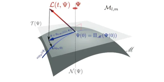
Fig. 2 Geometric interpretation of the DO approximation and of the exponential map expR. The
time derivative \scrL (t, R) is replaced by its best tangent approximation. Schematic adapted from Wikimedia Commons, https:// commons.wikimedia.org/ wiki/ file:tangentialvektor.svg.
be the dynamical system on M geometrically obtained by replacing the vector field
\scrL (t, \cdot ) with its tangent projection [17, 30]: (20)
\biggl\{ \.
\Psi = \Pi \scrT (\Psi )(\scrL (t, \Psi )), \Psi (0) = \Pi M(\Psi (0)),
where the notation \Pi M denotes the orthogonal projection onto the manifoldM and
\Pi \scrT (\Psi ) the orthogonal projection onto its tangent space at the point \Psi (see Figure 2). Given the choices (18) and (19), the ODE system (20) can be written as a set of coupled evolution equations for the mode and coefficient matrices U and Z that turn out to be exactly a discrete version of the continuous DO equations (14) and (15): (21)
\biggl\{ \.
Z = \scrL (t, U ZT)TU,
\.
U = (I - U UT)\scrL (t, U ZT)Z(ZTZ) - 1.
The orthogonal projection \Pi M ontoM used for the initialization of \Psi (0) is nothing
more than the application that maps the matrix \Psi onto its best rank-r\Psi
approx-imation, i.e., the truncated SVD [27] (this approach was used to initialize ocean uncertainty predictions [40, 38]). The SVD of the original numerical solution is the
discrete analogue of the Karhunen--Lo\`eve decomposition:
\Psi =
rank(\Psi )
\sum
i=1
\sigma i(\Psi )uivTi ,
where \sigma 1(\Psi ) \geq \cdot \cdot \cdot \geq \sigma rank(\Psi )(\Psi ) > 0 are the singular values of \Psi , and ui and vi
are orthonormal families of left and right singular vectors. The truncated SVD is the
algebraic operation that removes modes of order higher than r\Psi :
(22) \Pi M(\Psi ) =
r\Psi
\sum
i=1
\sigma i(\Psi )uivTi \in M .
Feppon and Lermusiaux [17] have shown that the dynamical system (20) instanta-neously applies the truncated SVD to constrain the rank of the reduced solution \Psi at
all times. In other words, it is the continuous limit when \Delta t \rightarrow 0 of the solution that would be obtained by systematically applying the truncated SVD after any Euler (or any other explicit time discretization) time step:
(23) \Pi \scrT (\Psi )(\scrL (t, \Psi )) = lim \Delta t\rightarrow 0
\Pi M(\Psi + \Delta t\scrL (t, \Psi )) - \Psi
\Delta t .
Therefore, (20) yields an optimal time evolution of the modal decomposition \Psi = U ZT
at least for small integration times. More theoretical guarantees have been obtained in [17], where it is proven that the error of the DO approximation (20) is controlled by the best truncation error | | \Psi (t) - \Pi M(\Psi (t))| | as long as the original solution \Psi (t)
remains at a close distance from the set M of low-rank matrices, which translates
into the algebraic condition
\sigma r\Psi (\Psi (t)) > \sigma r\Psi +1(\Psi (t));
i.e., singular values of order r\Psi and r\Psi +1 do not cross (a condition previously observed
numerically in [30, 52]).
3. Implementation of the DO Approximation for Stochastic Advection.
Ex-ploiting the geometric framework, new schemes for the DO approximation (21) of the stochastic transport equation (6) are obtained. High-order linear stabilized ad-vection schemes that maintain sharp spatial gradients and deterministic-stochastic consistency are presented (subsection 3.1). Stochastic DO BCs derived from opti-mality criteria are discussed (subsection 3.2). Time-marching strategies for the DO equations, using the truncated SVD and the retractions [1] for maintaining the nu-merical solution on the low-rank manifold, are obtained and contrasted: direct Euler, exponential map from geodesic equations, and algebraic and gradient descent--based time-marching (subsection 3.3). Finally, accurate methods for dynamically evolving the rank of the DO subspace and for preserving the orthonormality of the modes and their smooth evolution are derived (subsections 3.4 and 3.5).
3.1. Motivations for Linear Advection Schemes. The DO approximation is
computationally attractive because (21) evolves a solution constrained to the low-rank
manifold of small dimension (l + m)r\Psi - r\Psi 2(by evolving the lr\Psi + mr\Psi coefficients
of the matrices U and Z with U orthonormal), instead of the initial lm independent
matrix coefficients of the original high-dimensional dynamical system (17). As a
consequence, the DO matrix system (21) offers a true gain of computational efficiency only if the evaluation of l-by-m matrices can be avoided. This is not a priori achievable in a direct nonintrusive scheme if the operator \scrL needs to be evaluated on the l-by-m
matrix \Psi = U ZT. If all lm coefficients of \Psi were needed to be computed from U
and Z, there would be no computational benefit other than a reduction of memory storage in comparison with solving the original nonreduced system (17). The gain
of efficiency can be achieved if the operator \scrL (t, \cdot ) maps a rank-r\Psi decomposition
\Psi = U ZT onto a factorization
(24) \scrL (t, U ZT) = L
ULTZ
of rank at most rL, where LU is an l-by-rL matrix, LZ an m-by-rL matrix, and rL
an integer typically largely inferior to l and m. In that case, the system (21) can be computed efficiently as (25) \biggl\{ \. Z = LZ[LTUU ], \. U = [(I - U UT)L U][LTZZ(ZTZ) - 1],
where brackets have been used to highlight products that allow us to compute the
derivatives \.U and \.Z without having to deal with l-by-m matrices. Such factorization
occurs for instance when \scrL (t, \cdot ) is polynomial of order d, for which rank-r\Psi matrices
are mapped onto rank-rL\leq (r\Psi )d matrices.
From the spatially continuous viewpoint, the differential operator \bfitpsi \mapsto \rightarrow \bfitv \cdot \nabla \bfitpsi
satisfies this condition, as the rank-r\Psi decomposition (7) is mapped to one of rank
rL= r\Psi \times r\bfitv :
(26) \bfitv \cdot \nabla \bfitpsi = \sum
1\leq j\leq r\Psi 1\leq k\leq r\bfitv
\zeta j\beta k\bfitv k\cdot \nabla \bfitu j.
This equation further highlights why adapting advection schemes to model order reduction is challenging, as popular discretizations of \bfitv \cdot \nabla \bfitpsi involve nonpolynomial nonlinearities in the matrix operator \scrL . These schemes rely indeed on the use of min-max functions required by upwinding or high-order discretizations such as ENO or TVD schemes that select a smooth approximation of the spatial derivative \nabla \bfitpsi , e.g., [77]. In these cases, the nonlinearity of the operator \scrL prevents the decomposition (26) from holding at the discrete level without introducing further approximations, which may drastically alter the stability of time integration and the accuracy of the numerical solution. A very natural approach followed by [63, 80] is to assume that the decomposition (26) holds before applying nonlinear schemes to discretize the fluxes
\bfitv k \cdot \nabla \bfitu j in (14) and (15). A key issue then is to maintain consistency between the
deterministic MC and stochastic DO solutions. Indeed, in the examples considered in section 4, for which high gradients occur, such approaches were at times observed to lead to either numerical explosion or significant errors for long integration times.
Consequently, this work investigated the use of linear central advection schemes that do not require upwinding and that have the property of preserving the decom-position (26). Therefore, the advection - \bfitv \cdot \nabla \bfitpsi is discretized as
(27) \scrL (t, \Psi )i,\alpha = - \bfitv (t, \bfitx i; \omega \alpha ) \cdot D\Psi i,\alpha ,
where D is a linear finite-difference operator approximating the gradient \nabla . With
\Psi = U ZT as in (18), this yields the decomposition \scrL (t, \Psi ) = L
ULTZ, as required in
(25), where LU and LZ are the l-by-rL and m-by-rL matrices
(LU)i,jk= \bfitv k(t, \bfitx i) \cdot D\bfitu j(t, \bfitx i), (LZ)\alpha ,jk= \zeta j(t; \omega \alpha )\beta k(t, \omega \alpha ).
In one dimension, the gradient can be approximated by the second-order operator
(28) D\Psi i,\alpha =
\Psi i+1,\alpha - \Psi i - 1,\alpha
2\Delta x ,
and this article will also consider the sixth-order finite-difference operator (29) D\Psi i,\alpha =
3 2
\Psi i+1,\alpha - \Psi i - 1,\alpha
2\Delta x -
3 5
\Psi i+2,\alpha - \Psi i - 2,\alpha
4\Delta x +
1 10
\Psi i+3,\alpha - \Psi i - 3,\alpha
6\Delta x ,
where \Delta x denotes the spatial resolution, and a natural numbering is assumed for the index i. These formulas are adapted in a straightforward manner to discretize partial derivatives in higher dimension [54]. This approach might seem unexpected, since central schemes are known to be numerically unstable under Euler time integration. In addition, the Godunov theorem says that it is not possible to devise a linear
scheme higher than first-order accuracy that does not create false extrema in numerical solutions [18]. These extrema are produced by numerical dispersion and manifest in the form of spurious oscillations. In fact, it is possible to contain this phenomenon near shocks and obtain high-order accuracy where the solution is smooth. Stability and the removal of part of the oscillations can be achieved by introducing the right amount of numerical dissipation, using either artificial viscosity [72] or filtering [68, 14, 32, 59, 11]. Shapiro filters are especially attractive because they are easy to implement, fully linear, and designed to optimally remove the shortest resolvable numerical frequency
without affecting other wave components [68, 69, 70]. In one dimension, setting \delta 2as
the operator \delta 2\Psi i,\alpha = \Psi i+1,\alpha - 2\Psi i,\alpha + \Psi i+1,\alpha , the Shapiro filters \scrF (i)of order i = 2,
4, and 8 are defined by the formulas (see [68])
(30)
\scrF (2)\Psi
i,\alpha = (1 + \delta 2/4)\Psi i,\alpha ,
\scrF (4)\Psi
i,\alpha = (1 - \delta 2/4)(1 + \delta 2/4)\Psi i,\alpha ,
\scrF (8)\Psi
i,\alpha = (1 + \delta 4/16)(1 - \delta 4/16)\Psi i,\alpha .
The order and frequency of applications can be tuned to the desired filter spectrum [34]. Their linearity allows us to filter the decomposition \bfitpsi = \zeta i\bfitu i efficiently by
fil-tering the discretization of the modes \bfitu ior, in other words, \scrF (i)(U ZT) = (\scrF (i)U )ZT.
Critically, this DO filtering is consistent with the filtering of MC realizations. To achieve further stability, higher-order discretizations of the temporal derivative are generally used to complement these filters. Popular linear multistep methods are leapfrog [83], Runge--Kutta, and Adam Bashforth [11]. For instance, for a time
increment \Delta t, the second-order leapfrog scheme evolves the value \Psi nof the numerical
solution \Psi at time tn= n\Delta t according to the rule
(31) \Psi
n+1 - \Psi n - 1
2\Delta t = \scrL (t
n, \Psi n),
while the third-order Runge--Kutta (RK3) method uses
(32) \Psi n+1 - \Psi n \Delta t = kn 1 + 4k2n+ kn3 6 with \left\{ kn 1 = \scrL (tn, \Psi n), kn
2 = \scrL (tn+ \Delta t/2, \Psi n+ kn1\Delta t/2) ,
kn
3 = \scrL (tn+ \Delta t, \Psi n+ \Delta t(2k2n - kn1)).
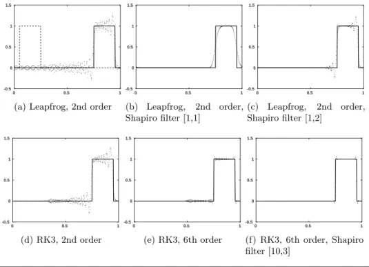
A comparison of several combinations of these techniques is illustrated in Figure 3 for the 1D advection equation \partial t\bfitpsi + v\partial x\bfitpsi = 0, a benchmark case for selecting an
appropriate linear scheme for the transport equation (6) in higher dimension. A
boxcar function is advected to the right with velocity v = 0.7 in the domain [0, 1] until time t = 10. The spatial resolution is set to \Delta x = 0.002, and the CFL condition \Delta t \leq 0.6v\Delta x is used to define the time increment \Delta t. The figure illustrates how accuracy and stability can be achieved by (i) using multistep time-marching schemes, (ii) using high-order spatial discretization, and (iii) adding the proper amount of numerical dissipation to remove spurious oscillations. We note that linear limiters may also be combined with Shapiro filters [24], maintaining consistency.
3.2. Boundary Conditions. BCs of the reduced solution were formally obtained
in section 2. They could be treated more rigorously by incorporating the original BCs, (8) and (9), directly within the discretization of the operator \scrL . However, this approach can lead to a more complex implementation. In this work, boundary nodes
are stored in an lbc-by-m ``ghost"" matrix, and it is assumed that the l-by-m matrix
of realizations \Psi contains only the values at internal nodes. These ghost cells allow
0 0.5 1 -0.5 0 0.5 1 1.5
(a) Leapfrog, 2nd order
0 0.5 1 -0.5 0 0.5 1 1.5 (b) Leapfrog, 2nd order, Shapiro filter [1,1] 0 0.5 1 -0.5 0 0.5 1 1.5 (c) Leapfrog, 2nd order, Shapiro filter [1,2] 0 0.5 1 -0.5 0 0.5 1 1.5 (d) RK3, 2nd order 0 0.5 1 -0.5 0 0.5 1 1.5 (e) RK3, 6th order 0 0.5 1 -0.5 0 0.5 1 1.5 (f) RK3, 6th order, Shapiro filter [10,3]
Fig. 3 Comparison of the numerical solution ( dotted line) with the analytical solution ( solid line) of
the 1D advection equation for different time-integration, linear centered schemes, and filter
order (specifics given in each panel caption). The text ``Shapiro filter [n1, n2]"" indicates that
the Shapiro filter of order 2n2 (see [68]) has been applied after every n1 iterations. The
initial boxcar function is visible in the dashed line on the first plot.
convenient evaluation of the differential operator D in the definition (27) of \scrL (t, \Psi ). Their values are reinitialized at the beginning of each time step according to the BCs (8) and (9). In the following, the operator which assigns the values of these boundary
cells at time t is denoted \scrB C(t, \cdot ); i.e., the discrete BCs are then explicit (if implicit,
they are solved for simultaneously with the interior solution, e.g., see [21]). With this notation, the solution that includes both internal nodes and boundary values is the block matrix \Psi bc=\bigl[ \scrB C(t,\Psi )\Psi \bigr] . For example, on the 1D domain \Omega = [0, 1], the value
of the boundary node \bfitx 1= 0 is determined by the relation
\scrB C(t, \Psi )1,\alpha =
\biggl\{
0 if \bfitv (t, 0; \alpha ) \geq 0,
(18\Psi 2,\alpha - 9\Psi 3,\alpha + 2\Psi 4,\alpha )/11 if \bfitv (t, 0; \alpha ) < 0,
if one uses a third-order reconstruction for the Neumann BC (9). The difficulty of
determining how these BCs should be accounted for by the reduced solution \Psi = U ZT
comes from the fact that assigning boundary values does not in general preserve
the rank; i.e., rank(\Psi bc) > r\Psi (in practice, the rank of this interior+boundary DO
solution should be large enough to represent both the reduced interior solution and the reduced BCs; see [21]). BCs may be enforced on the reduced solution while ensuring minimal error by solving the minimization problem
(33) min rank(\Psi bc)=r\Psi \bigm| \bigm| \bigm| \bigm| \bigm| \bigm| \bigm| \bigm| \Psi bc - \biggl[ \scrB C(t, \Psi ) \Psi \biggr] \bigm| \bigm| \bigm| \bigm| \bigm| \bigm| \bigm| \bigm| 2 .
This yields the best rank-r\Psi approximation of the (l + lbc)-by-m matrix \Psi bc, whose
decomposition \Psi bc= UbcZbcT allows us to conveniently compute the discrete differential
operator D in (27) requiring boundary values. The minimization can, e.g., be achieved
by using a gradient descent starting from the initial rank-r\Psi matrix \Psi , as explained
in the next subsection and in [17, 50].
When BCs are deterministic or homogeneous, they can be directly implemented
as BCs for the discretization of the modes \bfitu i [63]. For example, zero Dirichlet or
Neumann BCs for all the realizations of \bfitpsi directly corresponds to the same BCs for
the modes \bfitu i. For more general cases, it is usually desirable to avoid solving (33)
and to instead obtain BCs for the modes that optimally approximate the original BCs. This is achieved by replacing the minimization problem (33) with that for the
lbc-by-r\Psi ghost matrix Ubccontaining boundary values for the matrix U :
(34) min
Ubc\in \scrM lbc,r\Psi
| | UbcZT - \scrB C(t, \Psi )| | 2.
The solution of this linear regression problem is easily obtained by writing the sta-tionarity condition
\forall \delta U \in \scrM lbc,r\Psi , 2\langle (\delta U )Z T, U
bcZT - \scrB C(t, \Psi )\rangle = 0,
which eventually yields
(35) Ubc= \scrB C(t, \Psi )Z(ZTZ) - 1.
It turns out that this optimality condition is the discrete analogues of the original BCs (16) obtained formally in section 2. The decomposition of the reduced solution
including boundary values is therefore \Psi bc = \bigl[ UUbc\bigr] ZT. Further discussions on DO
BCs are provided in [21].
3.3. Low-Rank Time-Stepping. One issue commonly encountered in the time
discretization of dynamical systems is the fact that the discrete time-stepping tends
to make the numerical solution exit the manifold M where the trajectories live. If
\Psi n is a point on the manifold M at tn, and \.\Psi n \in \scrT (R) is the time derivative,
any straight move, \Psi n+ \Delta t \.\Psi n, leaves the fixed-rank manifoldM . An application,
called retraction, must be used to convert the tangent direction X = \Delta t \.\Psi n\in \scrT (\Psi n)
into a point \rho \Psi n(X) back onto the manifold. A retraction \rho \Psi n : \scrT (\Psi n) \rightarrow M
(Figure 2) is an application describing how to move on the manifold in a tangent
direction X \in \scrT (\Psi n) starting from \Psi n \in M . By definition, it must satisfy the
consistency conditions that (i) zero velocity results in a null move, i.e., \rho \Psi n(0) = \Psi n,
and (ii) a move in the X direction results in a trajectory on M with X as initial
speed: dtd\rho \Psi n(tX)\bigm| \bigm| t=0= X (see [1]). The ideal retraction is the exponential map that follows geodesics or shortest paths on the manifold but may be expensive to evaluate. In practice, one uses approximations of this map, leading to several strategies of implementation for the explicit discretization of (21).
3.3.1. Direct Time-Marching Scheme for the Matrix DO System (21). As in
[80, 52], a very intuitive idea for moving a rank-r\Psi matrix \Psi n = UnZnT onto a
direction \.\Psi n = \.UnZnT+ UnZ\.nT with a step \Delta t is to independently update the mode
and coefficient matrices Un and Zn by using the following scheme, which is a direct
Euler time discretization of the system (21):
(36) \biggl\{ Z
n+1= Zn+ \Delta t \.Zn,
Un+1= Un+ \Delta t \.Un,
where \.Znand \.Un are the approximations of the time derivatives \.U and \.Z being used.
This corresponds to using the retraction \rho U ZT defined by
(37) \rho U ZT( \.U ZT + U \.ZT) = (U + \.U )(Z + \.Z)T = U ZT + ( \.U ZT + U \.ZT) + \.U \.ZT.
3.3.2. The Exponential Map: Geodesic Equations between Time Steps. The
ideal retraction is the exponential map \rho \Psi n = exp\Psi n (see [1]) computed from geodesic
paths \gamma (s) onM , which are the direct analogues of straight lines onto curved
man-ifolds. These curves, parametrized as \gamma (s) = exp\Psi n(s
.
\Psi n) (see Figure 2), indicate
the shortest way to ``walk"" onto the manifold from \Psi n in the straight direction
.
\Psi n = \.Un(Zn)T + Un( \.Zn)T. The value of exp
\Psi n(s .
\Psi n) is given by the solution
\gamma (s) = U (s)Z(s)T at time s of the geodesic equations [17]:
(38) \left\{ \" Z - Z \.UTU = 0,\. \" U + U \.UTU + 2 \.\. U \.ZTZ(ZTZ) - 1= 0, U (0) = Un, Z(0) = Zn, \. U (0) = \.Un, \.Z(0) = \.Zn.
Without direct analytical solutions to (38), numerical schemes are used. Computing retractions that approximate the exponential map well is a challenge commonly en-countered in optimization on matrix manifolds with orthogonality constraints [50], as
discussed in [1]. One can show that the retraction \rho U ZT of equation (37) approximates
the exponential map only to first order (see [1]), which can lead to numerical errors
at locations of high curvature on the manifold M . The curvature of the rank-r\Psi
manifold M at the point \Psi n is inversely proportional to the lowest singular value
\sigma r\Psi (\Psi
n) [17]. As a consequence, errors can be incurred by the direct time-stepping
(36) when the matrix Zn is ill conditioned. Equations (38) can be solved during the
DO time integration between time steps to move more accurately on the manifold without needing to recompute values of the operator \scrL . For instance, Euler steps (36) can be replaced with
(39) Un+1(Zn+1)T = exp\Psi n(\Delta t
.
\Psi n).
This can be done using high-order time-marching schemes for the discretization of (38). The intermediate time step \delta t < \Delta t for these can be set adaptively: a rule of thumb is to use steps in the ambient space having a length less than the minimal curvature radius \sigma r\Psi (Z) at the point U Z
T:
\delta t| | \.U ZT+ U \.ZT| | < C\sigma r\Psi (Z),
where C \simeq 1 is a constant set by the user. Note that a lower-order retraction such as (37) is commonly used anyway in the time discretization of the geodesic equations (38).
3.3.3. Direct Computation of the Truncated SVD at the Next Time Step. As
highlighted in section 2, DO equations (25) define a dynamical system that truncates the SVD at all instants to optimally constrain the rank of the reduced solution (23).
Denoting \Psi n = Un(Zn)T as the DO solution at time tn, integrating the nonreduced
dynamical system (17) for a time step [tn, tn+1] yields a rank-r
L> r\Psi prediction
(40) \Psi n+1= \Psi n+ \Delta t\scrL (tn, \Psi n),
where \scrL (tn, \Psi n) represent the full-space integral for the exact integration or the
incre-ment function for a numerical integration. For the latter, it can be an approximation of the time derivative \scrL (tn, \Psi (tn)), e.g., \scrL (tn, \Psi n) = \scrL (tn, \Psi n) for explicit Euler.
One way to proceed to evolve the low-rank approximation \Psi n to \Psi n+1 is to
directly compute the rank-r\Psi SVD truncation \Pi M(\Psi n+1) (equation (22))
(41) \Psi n+1= Un+1(Zn+1)T = \Pi M(\Psi n+ \Delta t\scrL (tn, \Psi n))
to obtain modes and coefficients Un+1 and Zn+1 at time tn+1 = tn + \Delta t. This
scheme has been shown to be a consistent time discretization of the DO equations
(20) (see [17]). For an Euler step, it corresponds to using the retraction \rho \Psi (X) =
\Pi M(\Psi + X), a second-order accurate approximation of the exponential map [1] and
hence an improvement of the direct Euler time-marching (36).
a. Algebraically Computing the Truncated SVD. The scheme (41) can be
com-puted efficiently and in a fully algebraic manner when the operator \scrL factors as (24). Indeed, the linear approximation of the time derivative then admits a decomposition \scrL (tn, Un(Zn)T) = Ln
U(L n Z)
T of rank at most r
L = rL\times pt, ptbeing the order of the
time integration scheme utilized. Therefore, \Psi n+1 factors as
(42) \Psi n+1= Un(Zn)T+ \Delta tLn U(L n Z) T
= \Psi n+1U (\Psi n+1Z )T, with \Psi n+1U = [Un LnU] and \Psi n+1
Z = [Z
n \Delta tLn Z],
with LnU \in \scrM l,rL, LZn \in \scrM m,rL. The rank of \Psi n+1is therefore at most rank(\Psi n+1) =
r\Psi < r\Psi + rL, which can be assumed to be largely inferior to l and m. This can be
exploited to compute the truncated SVD through an algorithm that avoids computing large matrices of size l-by-m (see Algorithm 3.1a).
Algorithm 3.1a Rank-r\Psi truncated SVD of \Psi = \Psi U\Psi TZ with \Psi U \in \scrM l,r\Psi , \Psi Z \in
\scrM m,r\Psi and r\Psi < r\Psi = rank(\Psi ) \ll min(l, m)
1: Orthonormalize the columns of the matrix \Psi U (see the discussion in
subsec-tion 3.5), i.e., find a basis change matrix A \in \scrM r\Psi ,r\Psi such that (\Psi UA) T(\Psi
UA) =
I and set
\Psi U \leftarrow \Psi UA, \Psi Z \leftarrow \Psi ZA - T
to preserve the product \Psi = \Psi U\Psi TZ.
2: Compute the ``compact"" SVD of the smaller m-by-r\Psi matrix \Psi Z:
\Psi Z = V \Sigma PT,
where \Sigma is an r\Psi -by-r\Psi diagonal matrix of singular values, and V \in \scrM m,r\Psi and
P \in \scrM r\Psi ,r\Psi are orthogonal matrices of singular vectors. This is achieved by
computing the eigendecomposition of the ``covariance"" matrix \Psi T
Z\Psi Z.
3: The SVD of \Psi = \Psi U\Psi TZ is given by \Psi = U \Sigma VT, with U = \Psi UP an
orthog-onal l-by-r\Psi matrix of left singular vectors. The truncated SVD of order r\Psi is
straightforwardly obtained from the first r\Psi columns of U, V , and \Sigma .
This first algorithm has some issues. First, reorthonormalizations and eigenvalue decompositions such as in steps 1 and 2 do not allow us to keep track of the smooth evolution of the mode U (t) and coefficient Z(t) solutions of the system (21). Addi-tional procedures are needed [80, 79]. Second, with the repeated use of such algebraic operations, additional round-off errors may be introduced.
b. Using Gradient Descent for Continuous Updates of the Truncated SVD.
Alternatively, a gradient descent on the low-rank manifoldM can be used to find the
correction that needs to be added to modes Un and coefficients Zn to evaluate the
SVD truncation \Psi n+1= \Pi
M(\Psi n+1) ((41) and (42)). Indeed, \Psi n+1= Un+1(Zn+1)T
(eq. (41)) is the minimizer of
J (U ZT) = 1 2| | \Psi n+1 U (\Psi n+1 Z ) T - U ZT| | 2,
where | | \cdot | | is the Frobenius norm. The (covariant) gradient \nabla J used for this
mini-mization must be aligned with the maximum ascent direction tangent toM at UZT.
Its value can be shown to be \nabla J = (\nabla JU)ZT + U (\nabla JZ)T (see [17]), where \nabla JU
and \nabla JZ provide respective ascent directions for the individual matrices U and Z.
Their expression and the resulting gradient descent toward the updated truncated
SVD Un+1(Zn+1)T starting from the approximate initial guess \Psi n = Un(Zn)T are
detailed in Algorithm 3.1b. Note that [17] proved that the procedure is convergent for almost every initial data point. If, in addition, \Delta t is small enough, the method is expected to converge after only a small number of iterations, while preserving the con-tinuous evolution of the mode and coefficient matrices U and Z. In comparison with the use of geodesics, this method ensures the accuracy of the reduced solution while being less sensitive to the singularity of the matrix Z. Also, it is a direct extension of the DO time stepping (36), as one step of (36) coincides with the first step of the
gradient descent (43) starting from the current value Un(Zn)T and with \mu = 1 [17].
Algorithm 3.1b Gradient descent for updating a rank-r\Psi truncated SVD of \Psi =
\Psi U\Psi TZ with \Psi U \in \scrM l,r\Psi , \Psi Z\in \scrM m,r\Psi , and r\Psi < r\Psi = rank(r\Psi ) \ll min(l, m)
1: Initialize a rank-r\Psi guess U0Z0T \simeq \Psi with U0\in \scrM l,r\Psi , Z0\in \scrM m,r\Psi , U T
0U0= I.
2: To minimize J (U, Z) = J (U ZT) = | | \Psi - U ZT| | onM , compute the gradient step
(43) \biggl\{ Zk+1= Zk - \mu \nabla JU(Uk, Zk),
Uk+1= Uk - \mu \nabla JZ(Uk, Zk),
where \mu is a small enough constant set by the user and the gradients (\nabla JU, \nabla JZ)
are given by (see Proposition 36 in [17])
(44) \Biggl\{ \nabla JZ(U, Z) = Z - \Psi Z[(\Psi U)
TU ],
\nabla JU(U, Z) = - (I - U UT)\Psi U[(\Psi Z)TZ(ZTZ) - 1],
where brackets highlight matrix products that render the computation efficient.
3: Orthonormalize the modes Uk+1 (see subsection 3.5) after each iteration and
re-peat steps 2--3 until convergence is achieved.
3.4. Dynamically Increasing the Rank of the Approximation. In the SPDE
(6), all realizations of the solution share the initial value \bfitpsi (0, \bfitx ; \omega ) = \bfitx . Hence, the DO approximation coincides with the exact solution at time t = 0 and is given by
the rank-one decomposition \Psi = U ZT, where U is a normalized column vector
pro-portional to the discretization of the coordinate function \bfitx and Z is a column vector identically equal to the normalization factor. Obviously, \bfitpsi (t, \bfitx ; \omega ) becomes random after t > 0 and hence the rank of the DO solution must be increased immediately [64, 80] and modified dynamically to capture dominant stochastic subspaces that are
forming throughout the time evolution of the solution. This is a common issue in model order reduction of SPDEs.
Reducing the dimension r\Psi of the DO stochastic subspace is straightforward: it
is sufficient to truncate the SVD of the current DO solution \Psi = U ZT, using, i.e.,
Algorithm 3.1a, when the lowest singular value \sigma r\Psi (\Psi ) < \sigma becomes lower than a
threshold \sigma [64]. Increasing the stochastic dimension from r\Psi to r\Psi \prime > r\Psi is more
involved, as r\Psi \prime - r\Psi new dominant directions \bfitu i supporting the decomposition (7)
must be found. The overall topic is linked to breeding schemes [29]; directions of maximum error growth, e.g., [57]; and nonnormal modes [16, 15, 51], but our emphasis here is on accurately capturing the present and evolving dominant uncertainties in the SVD sense, as in [43, 35, 64]. One approach [64] assumes that uncertainties are small and uniform in the orthogonal complement of the present DO subspace and then adds modes aligned with the most sensitive directions of the operator \scrL in this complement, if their growth is fast enough. This computation is based on the gradient of \scrL in the
ambient space \scrM l,m, and MC perturbations, but it does not guarantee tracking the
best rank-r\Psi \prime approximation at the next time step. An additional difficulty lies in
the issue of detecting when the dimension of the DO subspace should be increased. Sapsis and Lermusiaux [64] suggested increasing the rank r\Psi when \sigma r\Psi (\Psi ) > \sigma reaches
another threshold, \sigma > \sigma .
These issues can be resolved by examining the component of the time derivative, \scrL (t, \Psi ), that is normal to the manifold, i.e., N (U ZT) = (I - \Pi
\scrT (U ZT))(\scrL (t, U ZT)) \in
\scrN (\Psi ), and neglected by the DO approximation (see Figure 2). The value of this component is given by (see Proposition 35 in [17])
(45) N (U ZT) = (I - U UT)\scrL (t, U ZT)(I - Z(ZTZ) - 1ZT).
Since the singular value \sigma r\Psi +1(\Psi
n+ \Delta tL(tn, \Psi n)) after a step \Delta t is of magnitude
\sigma 1(N (\Psi n))\Delta t (see [27]), this first and other singular values of N (U ZT) are related
to the speed at which the solution exits the rank-r\Psi matrix manifold M . Thus, a
quantitative criterion that can track the rank of the true original solution is
(46) \sigma 1(N (Un(Zn)T))\Delta t > \sigma .
A common value \sigma can be used for the threshold \sigma = \sigma = \sigma to detect when the rank of the DO subspace must be decreased/increased; hence the setting of this single \sigma provides the desired lower bound for the smallest singular value of the covariance
matrix Z. Singular vectors of N (Un(Zn)T) contain the new dominant directions.
They can be combined with a gradient descent similar to (43) to compute the rank-r\Psi \prime (instead of r\Psi ) truncated SVD of \Psi n+1= \Psi n+ \Delta tL(tn, \Psi n), while preserving the
smooth evolution of the first r\Psi modes and coefficients (in contrast with the direct
use of the algebraic Algorithm 3.1a). The procedure is summarized in Algorithm 3.2.
3.5. Preserving the Orthonormality of the Mode Matrix \bfitU . As highlighted
in [80], an issue with time discretization, e.g., (36) or (43), is that, in general, the
l-by-r\Psi matrix Un+1 \in \scrM l,r\Psi obtained after a discrete time step does not exactly
satisfy the orthogonality constraint Un+1TUn+1 = I. A numerical procedure must
therefore be used to reduce the truncation errors committed by the discretization,
even though the true trajectory U (t)ZT(t) onM and the DO equations (21) ensure
and assume UTU = I at all instants. This procedure must be accurate, as numerical
orthonormalization may also introduce round-off errors that can lead to significant error over large integration times. For example, standard and modified Gram--Schmidt
Algorithm 3.2 Augmenting the rank of the DO solution
1: Compute \Psi n+1 = Un(Zn)T + \Delta LnU(LnZ)T with LnU \in \scrM l,rL, LnZ \in \scrM m,rL as in
(42).
2: Compute the normal component (of rank at most rL) at tn:
N (Un(Zn)T) = [(I - Un(Un)T)LnU][(L n Z)
T
(I - Zn((Zn)TZn) - 1(Zn)T)]. 3: Compute the rank-r\Psi \prime - r\Psi < rLtruncated SVD of N (U
n(Zn)T) , i.e., Nn U(N
n Z)
T,
using Algorithm 3.1a.
4: Use the gradient descent (43) starting from the initialization values U0= [UnNUn]
and Z0 = [ZnNZn], to find the truncated SVD of rank r\Psi \prime > r\Psi of \Psi n+1, i.e.,
Un+1(Zn+1)T.
orthonormalization presents numerical instabilities when U ZT becomes close to
be-ing rank deficient (see [76]). For this reason, [79, 80] used the followbe-ing procedure:
compute the eigendecomposition of the Gram matrix K = UTU ,
(47) P KPT = \Sigma .
Then rotate and scale modes and coefficients accordingly by setting (48)
\biggl\{
U \leftarrow U P \Sigma - 1/2, Z \leftarrow ZP \Sigma 1/2.
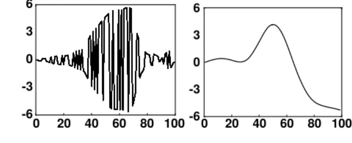
The eigenvalue problem (47) can be solved using Householder factorization, which is known to be numerically stable in comparison with Gram--Schmidt orthonormaliza-tion [76]. An issue is that this procedure may introduce permutaorthonormaliza-tions or sign changes, leading to artificial discontinuities in the time evolution of the mode and coefficient matrices U and Z. Figure 4 illustrates the problem by plotting the typical evolution of a coefficient of the matrix Z with this orthonormalization procedure. Even though sign checks alleviate the problem [80], they are a burden. Hence, to reinforce orthog-onality between time steps and provide smooth evolutions for both U and Z (21), one can employ a gradient flow, as was done in the DO time-stepping (43).
Reorthonor-malization is then performed by finding an invertible matrix A \in \scrM r\Psi ,r\Psi such that
(U A)T(U A) = ATKA = I and by setting U \leftarrow U A and Z \leftarrow ZA - T. Such a matrix
0 20 40 60 80 100 6 0 -3 -6 3 0 20 40 60 80 100 6 0 -6 -3 3
Fig. 4 Evolution of a coefficient of the matrix Zn obtained by the time integration of (21) as a
function of the iteration number. On the left, reorthonormalization of the matrix Un is
performed by solving the eigenvalue problem (48), while on the right, the gradient flow (49) was used. Eigenvalue decompositions introduce sign flips and permutations that result in
artificial discontinuities in the individual matrices Un and Zn if dealt with algebraically
[80].
A is actually the minimizer over \scrM r\Psi ,r\Psi of the functional
G(A) = 1
4| | A
TKA - I| | 2.
Therefore, one can find a reorthonormalization matrix A close to the identity by solving the gradient flow
(49) dA
ds = -
dG
dA = - KA(A
TKA - I)
with initial value A(0) = I. The inverse A - 1 of A can be simultaneously tracked by
solving the ODE
dA - 1
ds = - A
- 1dA
dsA
- 1.
The resulting numerical procedure is summarized in Algorithm 3.3. Typically, one
expects A = I + O(| | UTU - I| | ) and hence both corrections U A \simeq U and ZA - T \simeq Z
will have an order of magnitude identical to the initial error, ensuring the smooth evolution of U and Z. Figure 4 shows the time evolution of a coefficient of the matrix Z using this method. Only a few Euler steps are necessary to obtain convergence, which makes the method efficient. The matrix A \simeq I is well conditioned and the Algorithm 3.3 has small round-off errors.
Algorithm 3.3 Reorthonormalization procedure of U ZT \in M with UTU \simeq I
1: Define a tolerance parameter \epsilon and a time step \mu (typically \mu \simeq 1). 2: K \leftarrow UTU 3: A \leftarrow I, A - 1\leftarrow I 4: while | | AT kKAk - I| | 2> \epsilon do 5: dAk \leftarrow - KAk(ATkKAk - I) 6: Ak+1\leftarrow Ak+ \mu dAk
7: A - 1k+1\leftarrow A - 1k - \mu A - 1k (dAk)A - 1k
8: k \leftarrow k + 1
9: end while
10: U \leftarrow U Ak and Z \leftarrow ZA - Tk
4. Numerical Results.
4.1. Stochastic Double-Gyre Flow. The double gyre is the classic 2D benchmark
flow for the study of Lagrangian coherence of particle motions [67, 44, 25]. The
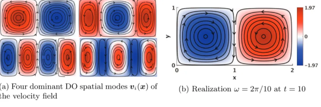
idealized flow consists of two vortices oscillating horizontally. Currently, the above new schemes are utilized to analyze how the Lagrangian motion of particles is affected by the oscillation angular frequency \omega . Hence, a range of initial \omega values is considered and \omega is modeled as an unknown random parameter. The classic analytical deterministic flow [67] then becomes stochastic (Figure 5):
\bfitv (t, \bfitx ; \omega ) = ( - \partial y\phi , \partial x\phi ) with \phi (\bfitx , t; \omega ) = A sin[\pi f (x, t; \omega )] sin(\pi y),
where f (x, t; \omega ) = \epsilon sin(\omega t)x2+ (1 - 2\epsilon sin(\omega t))x, \bfitx = (x, y), and \omega is initially random.
The fixed parameter values here are A = 0.1 and \epsilon = 0.1. The goal is to provide solutions to the SPDE (6), up to time t = 10 and for \omega uniformly distributed within [\pi /10, 8\pi /10].
(a) Four dominant DO spatial modes \bfitv i(\bfitx ) of
the velocity field
(b) Realization \omega = 2\pi /10 at t = 10
Fig. 5 Stochastic double-gyre flow with an initially random oscillation angular frequency.
Stream-lines are overlaid on the colored intensity of the vorticity.
For the DO computations, the spatial domain [0, 2] \times [0, 1] is discretized using
a 257 \times 129 grid with lbc = 2 \times 768 boundary nodes and the stochastic domain
[\pi /10, 8\pi /10] with m = 10,000 realizations \omega \alpha uniformly distributed according to
\omega \alpha = \pi 10+ \biggl( \alpha - 1 m - 1 \biggr) 7\pi
10, 1 \leq \alpha \leq m.
Hence, in this example, l = 2 \times (257 \times 129 - 768) = 64,770. The threshold used for
increasing the stochastic dimensionality (eq. (46)) is set to \sigma = 10 - 2. The retraction
used in the DO time-marching is that of subsection 3.3.3, computed with the gradient descent of Algorithm 3.1b.
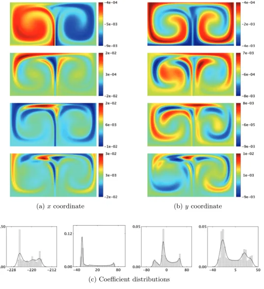
The stochastic velocity is decomposed into four time-independent modes \bfitv i(\bfitx )
(Figure 5), and coefficients \beta i(t; \omega ) = \langle \bfitv i(\bfitx ), \bfitv (t, \bfitx ; \omega )\rangle are obtained by orthogonal
projection. They force the SPDE (6). The initial value \bfitpsi (0, \bfitx ; \omega ) = \bfitx of the flow-map solution is shown in Figure 6.
(a) x coordinate (b) y coordinate
Fig. 6 Initial value \bfitpsi (0, \bfitx ; \omega ) = \bfitx of the advection equation (6).
To first validate the fully linear sixth-order-central, RK3, Shapiro filter scheme selected in subsection 3.1, the PDE (6) is first solved directly backward in time (for-ward flow-map) for a fixed value of \omega = 2\pi /10 until t = 10 and contrasted with the popular fifth-order WENO scheme combined with the TVDRK3 time-stepping [54]. The two solutions and their differences are shown in Figure 7. As expected from the 1D example (Figure 3), the fully linear scheme induces very small numerical errors near shocks, by either smearing or overshooting small details. Indeed, the two flow-map solutions are very comparable, which demonstrates the broad applicability of this fully linear scheme for advection (e.g., they are used in ocean modeling [34, 23, 22]). The scheme is therefore to solve the DO equations (21), as discussed in section 3.