HAL Id: hal-01381976
https://hal.archives-ouvertes.fr/hal-01381976
Submitted on 14 Oct 2016
HAL is a multi-disciplinary open access
archive for the deposit and dissemination of
sci-entific research documents, whether they are
pub-lished or not. The documents may come from
teaching and research institutions in France or
abroad, or from public or private research centers.
L’archive ouverte pluridisciplinaire HAL, est
destinée au dépôt et à la diffusion de documents
scientifiques de niveau recherche, publiés ou non,
émanant des établissements d’enseignement et de
recherche français ou étrangers, des laboratoires
publics ou privés.
Parallel Homology Computation of Meshes
Guillaume Damiand, Rocio Gonzalez-Diaz
To cite this version:
Guillaume Damiand, Rocio Gonzalez-Diaz. Parallel Homology Computation of Meshes.
Computa-tional Topology in Image Context, Jun 2016, Marseille, France. pp.53 - 64,
�10.1007/978-3-319-39441-1_6�. �hal-01381976�
Guillaume Damiand1 and Rocio Gonzalez-Diaz2
1
Univ Lyon, CNRS, LIRIS, UMR5205, F-69622 France
2
Universidad de Sevilla, Dpto. de Matem´atica Aplicada I, S-41012, Spain
Abstract. In this paper, we propose a method to compute, in paral-lel, the homology groups of closed meshes (i.e., orientable 2D manifolds without boundary) represented by combinatorial maps. Our experiments illustrate the interest of our approach which is really fast on big meshes and which obtains good speed-up when increasing the number of threads.
Keywords: Homology Groups Computation; 2D Combinatorial Maps; Parallel Algorithm.
1
Introduction
With the rapid increase of the amount of data produced in recent decades, avail-ability of efficient tools to analyze these data is of great importance. Homology computation is a basic tool that helps to identify connected components, holes and voids in the given data. Nevertheless, the design of efficient algorithms for computing homology on large data is still a challenging task nowadays.
In [11], two parallel algorithms to compute homology of large simplicial com-plexes on multicore machines and GPUs were presented. The given complex is decomposed into different partitions. A map from simplices to their boundaries and coboundaries is constructed. This step takes up the highest percentage of the total execution time. Then, parallel algebraic reductions of cells [8] that reduce the size of the chain complex while maintaining its homology are performed. The modification of boundaries and coboundaries is also time-consuming. Finally, re-duced chain complexes are merged together and algebraic reductions are then performed sequentially to compute the homology of the input complex.
In this paper, we use 2D combinatorial maps to represent meshes (i.e., ori-entable 2D manifolds) avoiding the time-consuming step of constructing and modifying boundaries and coboundaries of cells. Besides, instead of using alge-braic structures (i.e., chain complexes) our data structures are always combina-torial maps. The principle of our method is to merge, in parallel, the faces of the mesh while the topology is preserved. To achieve this goal, faces of the object are dispatched in clusters. Edges shared by two faces in the same cluster can be processed safely in parallel. The edges shared by two faces in different clus-ters are then processed sequentially. In order to test quickly (in almost constant time) if two adjacent faces can be merged, union find trees are used. At the end of the process, a minimal 2D combinatorial map gives a direct representation of homology generators of the given mesh.
Section 2 recalls the related material regarding combinatorial maps and ho-mology computation on these maps. Section 3 proposes a parallel algorithm to compute a minimal combinatorial map from which we can directly obtain ho-mology groups and generators. Some experimental and computational results are presented in Sect. 4. Finally, we summarize the paper with a brief discussion in Sect. 5.
2
Preliminary Notions
2.1 2D combinatorial maps
A 2D combinatorial map [9, 6], called 2-map, is a model of representation of a mesh, which is composed by i-cells: vertices or 0-cells associated with points, edges or 1-cells which link two vertices, and faces or 2-cells which are bounded by cycle of edges. Two cells are incident if one cell belongs to the boundary of
the other one; while two i-cells c1 and c2 are adjacent if it exists one (i −
1)-cell incident to both c1 and c2. Note that, in the meshes considered here, it is
possible to mix different types of faces. For example, we can find triangles and quadrangles in a same mesh. The mesh shown in Fig. 1(a), has 5 faces, 14 edges and 12 vertices. The 2-map shown in Fig. 1(b) describing such mesh has 20 darts.
f3 1 e 4 e 5 e f2 2 e e3 f4 v2 v1 f1 v3 6 e f5 e7 (a) 4 5 1 2 3 6 11 12 9 8 10 7 13 16 17 14 15 18 20 19 (b)
Fig. 1. (a) Example of a mesh. (b) The corresponding 2-map.
An edge e is dangling if it is adjacent to only one edge (like edge e6 in
Fig. 1(a)). In this case, one vertex incident to e is incident to no other edge than
e. An edge e0is isolated if it has no adjacent edge (like edge e7in Fig. 1(a)). Note
that an isolated edge is a special case of a dangling edge. In this case, the two
vertices incident to e0 are incident to no other edge than e0. An edge e00incident
to two different faces is called inner (like edge e1 in Fig. 1(a)). Such an edge is
necessarily not dangling, nor isolated. Reciprocally, a dangling or isolated edge is necessarily incident to only one face.
In a 2-map, the different elements of a mesh are encoded by darts and links between these darts. A dart is an orientation of an edge. If an edge separates two
faces, it is described by two darts in the 2-map which represent the two possible orientations of the edge. A dart belongs exactly to one vertex, one edge and one face, and thus each cell of the mesh is described by a set of darts in the 2-map. For example, in Fig. 1(b), we can see the 2-map which represents the mesh given in Fig. 1(a). This 2-map has 20 darts drawn in Fig. 1(b) as oriented numbered
segments. Vertex v1of the mesh is described by the set of darts {2, 5, 8, 12}; edge
e1 by {8, 11}, and face f1 by {11, 12, 13, 14, 15, 16, 17, 18}.
Note that a 2-map is equivalent to the well-known half-edge data structure [12, 10]. The main interest of combinatorial maps is that they can be defined in any dimension which allows us to envisage to extend this work in higher dimension.
A 2-map represents the topological part of the mesh, i.e. its subdivision into cells and all the incidence and adjacency relations between these cells. It is possible to associate information to cells thanks to the notion of attribute. We speak about i-attributes for information associated to i-cells (for example colors to faces, or mutexes to vertices).
Several operations are defined on 2-maps in order to build, traverse and update meshes. Among these operations, edge removal and edge contraction will be used in this paper in order to compute the homology of a mesh. The
removal of an inner edge (like edge e1in Fig. 1(a)) consists in removing the edge
from the mesh by merging its two incident faces. In Fig. 1(a), removing edge e1
will merge faces f1 and f4 in only one face with 9 edges. Removing a dangling
edge (like edge e6 in Fig. 1(a)) will also remove the vertex incident only to the
dangling edge (this avoid isolated vertex). In Fig. 1(a), removing edge e6 will
remove also vertex v3. Lastly removing an isolated edge will also remove its two
incident vertices (like edge e7 in Fig. 1(a)) and its incident face (because this
face was described by only this isolated edge and its two incident vertices). Edge contraction consists in contracting an edge by merging its two incident vertices
(when they exist). In Fig. 1(a), contracting edge e1will merge vertices v1and v2
in only one vertex, then face f1 becomes a pentagon with a dangling edge and
f4 a triangle.
2.2 Homology computation
Homology can be thought as a method for defining k-dimensional holes (con-nected components, tunnels, voids) in a given mesh. We can think in a cycle as a closed submanifold and a boundary as the boundary of a submanifold. Then, a homology class (which represents a hole) is an equivalence class of cycles modulo boundaries. Homology groups (i.e. the groups of homology classes) are defined from an algebraic structure called chain complex composed by a set of groups
{Ck}, where each Ck is the group of k-chains generated by all the k-cells, and
a set of homomorphisms {∂k : Ck → Ck−1}, called boundary operator,
describ-ing the boundaries of k-chains. This way, a k-dimensional homology generator (called Hk generator) is a k-cycle which is not the boundary of any (k + 1)-chain. Thus, in principle, the manipulation of the boundary operator is needed to compute homology.
An algorithm allowing to compute the minimal 2-map describing an initial mesh without boundary while preserving the homology is described in [7]. Its principles consist first in removing all the inner edges: this merges all the faces of the mesh in only one face. The second step removes all the dangling edges: a dangling edge is removed when it is found, and the possible path of dangling edges is followed in order to ensure that all the dangling edges are removed. For computing H0 generators, we keep in a stack one vertex for each isolated edge before to remove it from the 2-map. The last step of the algorithm consists in contracting all non-loop edges. This allows us to obtain the minimal representa-tion of the initial mesh with 1 vertex for each connected component which is not a sphere, plus some loops incident to these vertices depending on the amount of H1 generators of the corresponding mesh. Observe that we do not need to com-pute or store the boundary operator for computing the homology of the mesh. The resulting minimal 2-map gives a direct representation of homology genera-tors. H0 generators are directly obtained by the set of vertices in the stack plus the set of vertices in the 2-map; H1 generators are directly obtained by the set of edges in the 2-map which are all loops and H2 generators are directly obtained by the set of faces in the initial 2-map.
3
Parallel Algorithm
The goal of this section is to propose a parallel version of the previous algorithm allowing to compute the minimal 2-map corresponding to a given mesh. When writing a parallel algorithm, the main issue is the concurrent access of the shared memory. In order to allow efficient parallel access, we use here a distributed version of 2-maps.
A distributed 2-map M is a 2-map where darts are distributed in several clusters, each face of the 2-map belonging to exactly one cluster. To describe that a face belongs to a cluster, we associate all darts of this face with this cluster. In this way, clusters are sets of darts which form a partition of the set of all the darts, and which can also be seen as a partition of the set of all the faces
of the 2-map. An edge of M is said critical if it belongs to different clusters3,
otherwise it is said non-critical.
The main interest of a distributed 2-map is to allow to process in parallel the different clusters since they are independent. However, it allows only to process in parallel all the non-critical edges. This property is used in Algo. 1, the algorithm which is the parallel simplification of a given 2-map. This algorithm has four steps:
– step 1a and step 1b to remove the inner edges; 1a in parallel for non-critical edges (by cluster); 1b sequentially for the whole set of critical edges of the 2-map;
– step 2 to remove dangling edges in parallel (for the global 2-map);
3
Since an edge e in a 2-map without boundary is a set of two darts, e belongs to different clusters if its two darts belong to two different clusters.
– step 3 to contract non loop edges sequentially (for the global 2-map).
Algorithm 1: Parallel simplification of a closed mesh in its minimal rep-resentation.
Input: A distributed 2-map M representing a closed mesh.
Output: The minimal 2-map corresponding to M, computed in parallel. 1a parallel for each non-critical edge e of M (by cluster) do
if e is an inner edge then remove e;
1b foreach critical edge e of M (sequentially for the global 2-map) do if e is an inner edge then remove e;
2 parallel for each edge e of M (for the global 2-map) do while e is dangling do
if e is isolated then push one vertex of e in S ; Remove e; else
e0← one edge adjacent to e;
lock the vertex v incident to e and e0; remove e; e ← e0;
unlock v;
3 foreach edge e of M (sequentially for the global 2-map) do if e is not a loop then
contract e;
3.1 Inner edge removals
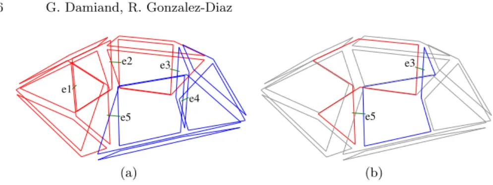
The step which does the inner edge removals is split in two parts (for non-critical edges and non-critical edges). Indeed, it is not possible to process in parallel the critical edge as illustrated in Fig. 2. In this example, a mesh representing a torus is simplified (cf. Fig. 2(a)). This 2-map has two different clusters (darts in the first cluster are drawn in red and darts in the second cluster in blue). After the removal of the three inner edges e1, e2 and e4, the 2-map shown in Fig. 2(b) is obtained. If edges e3 and e5 (which are criticals) are considered in parallel, they are both inner edges and thus they will be both removed. This would result in a wrong 2-map because the face resulting of the union of the 5 initial faces is not homeomorphic to a disk (here this is an annulus). Considering critical edges sequentially solves this problem: if e3 is considered, it is an inner edge and it is thus removed. Then when e5 will be considered, it will be no more an inner edge (because it will be incident twice to the same face) and thus it will be kept.
Note that this problem can not occur for non-critical edges (i.e. edges between two faces belonging to the same cluster). Indeed, in this case the two faces can be merged by only one thread, the one which processes this cluster. This justifies why we can process non-critical edges in parallel in step 1a of Algo. 1.
e1 e2 e3 e4 e5 (a) e5 e3 (b)
Fig. 2. Example of 2-map simplification illustrating why it is not possible to process critical edges in parallel for inner edge removal step. (a) Initial 2-map representing a torus. (b) 2-map obtained after the removal of the three inner edges of the initial 2-map e1, e2 and e4 (arrows on darts are not drawn in this figure).
For these two first steps, we avoid all the possible concurrent accesses because: – darts of different clusters are distributed in different containers in the 2-map. The parallel for each is done by associating one thread to each cluster, which allows to remove these darts in parallel during step 1a;
– critical edges (having two darts belonging to two different clusters) are pro-cessed sequentially.
3.2 Dangling edge removals
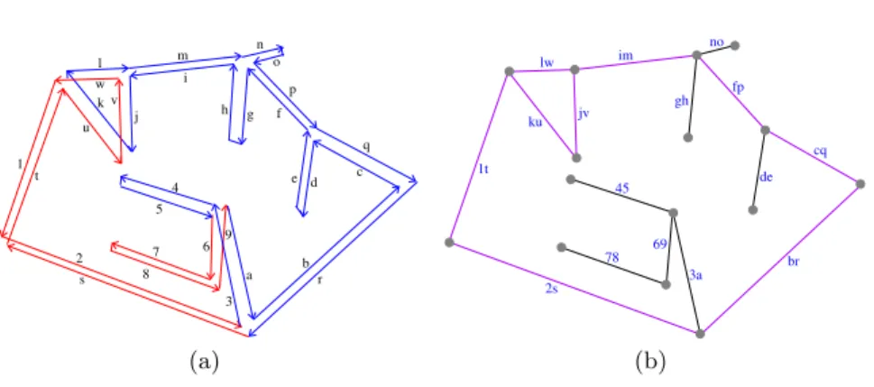
The same solution (process first non-critical edges in parallel then critical edges sequentially) can not be used for dangling edges, as illustrated in Fig. 3. This example shows the result of the two first steps of our simplification algorithm (steps 1a and 1b) on the mesh representing a torus (given in Fig. 2(a)). We have a 2-map having only one face (otherwise we would have some inner edges), some edges belong to H1 generators, i.e. to a cycle (in purple in Fig. 3(b)) but other edges do not (in black in Fig. 3(b)). The black edges need to be removed since they do not belong to H1 generators. This is done by the dangling edge removal step. In this example, all the edges 45, 78, gh, no and de are dangling and will be removed. However edges 69 and 3a are not yet dangling: they will become dangling after the removal of other dangling edges.
Two problems can arise if we want to process dangling edges in parallel cluster by cluster:
1. if two threads process edges in parallel (a first thread for red edges, a second for blue edges), we can consider simultaneously edges 45 and 69 (if the thread that processes red edges has already removed edge 78). If the two edges are removed simultaneously, the two threads will follow the path of dangling edges and they both will try to remove the same edge 3a;
2. to solve this problem, we can restrict each thread to process only the edges in its cluster. In this case, if edge 45 is considered by the blue thread before
8 n u 1 t 2 s 3 a br 7 6 5 4 9 c q d e f p o g h j v m i l w k (a) 1t ku jv lw im gh no fp de cq br 45 78 69 3a 2s (b)
Fig. 3. Example of dangling edge removal. (a) 2-map obtained from the initial 2-map given in Fig. 2(a) at the end of steps 1a and 1b. All inner edges were removed. Darts are labeled by numbers and letters. (b) Cellular representation representing by a graph all the vertices and edges of (a). Each edge of the graph is labeled by the two labels of its two darts in (a). Purple edges belong to H1 cycles while black edges not.
edge 69 by the red thread, the blue thread will not remove edge 3a because it is not yet dangling.
Our solution, given in Algo. 1 step 2 is to process all edges in parallel without taking into account the clusters. When a thread founds a dangling edge e, it removes e and follows the possible path of dangling edges starting from e. In order to avoid two threads to follow the same path, it is enough to add a mutex on each vertex of the 2-map, and to lock the mutex of the vertex which is not only incident to the dangling edge before removing the edge.
Now let us reconsider the previous example (given in Fig. 3) where two threads are processing edges 45 and 69 simultaneously. Only one thread will be able to lock the vertex {4, 6, a}; let us suppose it is the blue thread. This thread will remove edge 45, and then it will stop to follow the path of edges since the next edge in the path is not yet dangling. Then the second thread will now be able to take the mutex and will remove edge 69, but then the next edge 3a is dangling and it will be processed by this thread.
These mutexes solve the problem of concurrent access while guaranteeing that each edge that does not belong to an H1 generator will be removed. Indeed, these edges either belong to only one path of dangling edges (like edge 69 in the example) and these edges will be removed when the extremity of the path will be considered; or these edges belong to several paths (like edge 3a in the example) and these edges will be considered exactly once by the last thread that will take the mutexes of the vertices incident to the edges.
Lastly, darts are not directly deleted from the 2-map during this step be-cause the two darts of the current edge can belong to two different clusters, and two threads can want to delete simultaneously two darts belonging to the same cluster. Instead of adding mutexes on the containers of darts, we do not delete
the darts when dangling edges are removed but we only mark the darts to delete thanks to a specific Boolean mark. Then marked darts are deleted after having finished to process all dangling edges. These deletions can be done in parallel by iterating simultaneously through all the different containers.
3.3 Non loop edge contraction
The last step of Algo. 1 is the contraction of all the non-loop edges (an edge is a loop if it is incident twice to the same vertex). As we will see in our experiments in the next section, since this step is very fast (because the number of edges to contract is very small regarding the number of edges to remove), we decide in this work not to parallelize this step. Thus we use the classical algorithm which consists in iterating through each edge e, test if e is not a loop and contract it when it is the case.
4
Experiments
We have implemented our two algorithms, sequential and parallel version, by using the CGAL implementation of combinatorial maps [2] and the additional layer, called linear cell complex, which additionally represents the geometry [3].
All our experiments were run on an Intel i7-4790 CPU, 4 cores @ 3.60GHzR
with 32 Go RAM. We have tested our algorithms by comparing the sequential and the parallel version, and compared also our sequential version with RedHom [1]4.
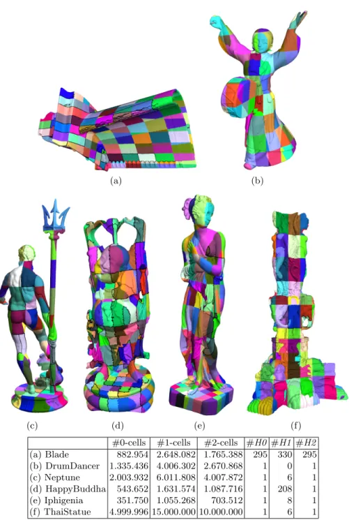
For our tests, we used the six meshes shown in Fig. 4, having between 703.512 and 10.000.000 faces. All these meshes have only one connected component, except Blade which has 295 connected components because it contains many small isolated closed meshes inside the blade. For the parallel algorithm, clusters are built during the load of the off files. We divide the bounding box of the mesh in 8 × 8 × 8 cubes, and fix the cluster of a face of the mesh depending on the cube which contains the minimal point of the face (these clusters are represented by different colors in Fig. 4).
Firstly we have compared our sequential algorithm and the sequential one implemented in RedHom. As we can see in Fig. 5(a), our method is much faster than RedHom: 22 times faster in average, the minimum gain is 3, 3 times for DrumDancer, and the maximum gain is 97 times for Blade. We observe that RedHom requires more time for meshes with big genus and/or big number of connected components while the complexity of our method is only related to the number of cells and not to the genus nor to the number of connected components. Secondly we have compared our two algorithms: the sequential and the par-allel one. For the parpar-allel version, we used eight threads because we ran the tests in a four core CPU, but with hyper-threading enabled. As we can observe in
4
We did not compare our solution with [11] because we were not able to compile their parallel version.
(a) (b)
(c) (d) (e) (f)
#0-cells #1-cells #2-cells #H0 #H1 #H2 (a) Blade 882.954 2.648.082 1.765.388 295 330 295 (b) DrumDancer 1.335.436 4.006.302 2.670.868 1 0 1 (c) Neptune 2.003.932 6.011.808 4.007.872 1 6 1 (d) HappyBuddha 543.652 1.631.574 1.087.716 1 208 1 (e) Iphigenia 351.750 1.055.268 703.512 1 8 1 (f) ThaiStatue 4.999.996 15.000.000 10.000.000 1 6 1
Fig. 4. The six meshes used in our experiments. Colors show the different clusters. Black curves show the H1 generators computed by our algorithm. The table gives the number of i-cells, #i-cells, and the number of Hi generators, #Hi, for i = 0, 1, 2.
0 5 10 15 20 25
Neptune Blade DrumDancer HappyBuddhaIphigenia Statuette
Time (sec) RedHom Sequential 4.29 23.3 1.74 3.60 0.55 10.7 1.06 0.24 0.52 0.19 0.11 1.95 (a) 0 0.2 0.4 0.6 0.8 1 1.2 1.4 1.6 1.8 2
Neptune Blade DrumDancer HappyBuddhaIphigenia Statuette
Time (sec) Sequential Parallel 1.06 0.24 0.52 0.19 0.11 1.95 0.35 0.14 0.19 0.09 0.06 0.68 (b)
Fig. 5. (a) Comparison of the times for the homology computation between RedHom and our sequential version. (b) Comparison of the times for the homology computation between our sequential and parallel versions (8 threads for the parallel version).
Fig. 5(b), the parallel version is in average 2, 4 times faster than the sequential one, the minimum gain is 1, 7 times for Blade and the maximum gain is 3 times for Neptune. We observe that the gain is better for bigger time of the sequen-tial algorithm, while this gain becomes small for very small time. However, this result is interesting because it is more important to speed up the bigger times than the smaller ones.
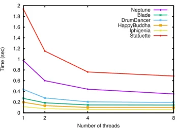
This result was confirmed by our next experiment where we have used our parallel algorithm by progressively increasing the number of threads from 1 to 8. The results shown in Fig. 6 confirm that the gain is more important when the time is bigger.
In order to study more precisely our algorithm, we have computed the number of edges contracted and removed during the different parts of our algorithms, both for the sequential version and the parallel version. Results are given in Table 1. Firstly we can see that the biggest number of edges is for the inner edge removal step (S1 and P1a), and the second biggest number is for the dangling edge removal step (S2 and P2). This justifies the interest of parallelizing these two steps. Secondly we can see that the number of critical edges processed by the parallel algorithm is very small as well as the time spend by this step (P1b). This shows that our solution to process these edges sequentially does not penalize the efficiency of our method. Lastly, we can see that the number of contracted edges is small as well as the time spend by this step (S3 and P3) which shows that the interest of parallelizing this step is less important (even if we can probably have a small gain here).
5
Conclusion
In this paper, we propose a parallel algorithm for computing the homology of orientable 2D manifolds without boundary represented by a 2-map. Our
0 0.2 0.4 0.6 0.8 1 1.2 1.4 1.6 1.8 2 1 2 4 8 Time (sec) Number of threads Neptune Blade DrumDancer HappyBuddha Iphigenia Statuette
Fig. 6. Times for the homology computation depending on the number of threads: 1, 2, 4 and 8. Sequential Parallel S1 S2 S3 P1a P1b P2 P3 Blade 1.765.093 857.663 24.996 1.764.486 607 858.825 23.834 DrumDancer 2.670.867 1.335.435 0 2.669.774 1.093 1.335.435 0 Neptune 4.007.871 1.991.051 12.880 4.006.454 1.417 1.998.477 5.454 HappyBuddha 1.087.715 531.494 12.157 1.085.360 2.355 529.280 14.371 Iphigenia 703.511 350.189 1.560 702.319 1.192 350.693 1.056 Statuette 9.999.999 4.994.414 5.581 9.991.484 8.515 4.995.786 4.209 Mean 3.372.509 1.676.708 9.529 3.369.980 2.530 1.678.083 8.154 Time 0.363s 0.278s 0.077s 0.113s 0.009s 0.093s 0.078s
Table 1. Number of edges removed and contracted during the different steps of our algorithms, comparing the sequential and the parallel ones (8 threads for the parallel version). The different steps are: for the sequential algorithm: S1 is the inner edge removal, S2 is the dangling edge removal, S3 is the edge contraction; for the parallel algorithm: P1a is the inner edge removal of non critical edges, P1b is the inner edge removal of critical edges, P2 is the dangling edge removal and P3 is the edge contraction. All the rows give the number of removed or contracted edges, except the last line which gives the time (in seconds). The last two lines are the means for the six meshes.
periments illustrate that the implemented version of the algorithm is computa-tionally convenient on big meshes and with good speed-up when increasing the number of threads.
We plan to extend our work to non-orientable manifolds once the package implementing generalized maps will be integrated in CGAL. Another possible extension is the parallel homology computation on manifolds with boundary. Probably we will need to add to the algorithm a special case for border edges. Finally, extension in nD could be given based on the theoretical results for removal and contraction operations in any dimension given in [4, 5].
Acknowledgments. This research was partially supported by Spanish project MTM2015-67072-P and by the French National Agency (ANR), project SoL-StiCe ANR-13-BS02-0002-01. We also thank the anonymous reviewers for their valuable comments.
References
1. Redhom. http://redhom.ii.uj.edu.pl/.
2. G. Damiand. Combinatorial maps. In CGAL User and Reference Manual. 3.9 edition, 2011. http://www.cgal.org/Pkg/CombinatorialMaps.
3. G. Damiand. Linear Cell Complex. In CGAL User and Reference Manual. 4.0 edition, 2012. http://www.cgal.org/Pkg/LinearCellComplex.
4. G. Damiand, R. Gonzalez-Diaz, and S. Peltier. Removal operations in nD gener-alized maps for efficient homology computation. In Proc. of 4th Int. Workshop on Computational Topology in Image Context (CTIC), volume 7309 of LNCS, pages 20–29, Bertinoro, Italy, May 2012. Springer Berlin/Heidelberg.
5. G. Damiand, R. Gonzalez-Diaz, and S. Peltier. Removal and contraction operations in nD generalized maps for efficient homology computation. CoRR, abs/1403.3683, 2014.
6. G Damiand and P. Lienhardt. Combinatorial Maps: Efficient Data Structures for Computer Graphics and Image Processing. A K Peters/CRC Press, 2014. 7. G. Damiand, S. Peltier, and L. Fuchs. Computing homology for surfaces with
generalized maps: Application to 3D images. In Proc. of 2nd Int. Symposium on Visual Computing (ISVC), volume 4292 of LNCS, pages 235–244, Lake Tahoe, Nevada, USA, November 2006. Springer Berlin/Heidelberg.
8. T. Kaczy´nski, M. Mrozek, and M. ´Slusarek. Homology computation by reduction of chain complexes. Computers & Mathematics with Applications, 35(4):59 – 70, 1998.
9. P. Lienhardt. N-Dimensional generalized combinatorial maps and cellular quasi-manifolds. Inte. J. of Computational Geometry and Applications, 4(3):275–324, 1994.
10. M. M¨antyl¨a. An Introduction to Solid Modeling. Computer Science Press, 1988. 11. N.A. Murty, V. Natarajan, and S. Vadhiyar. Efficient homology computations on
multicore and manycore systems. In High Performance Computing (HiPC), 2013 20th International Conference on, pages 333–342, Dec 2013.
12. K. Weiler. Edge-based data structures for solid modeling in curved-surface envi-ronments. Computer Graphics and Applications, 5(1):21–40, 1985.