Density variations in the lower thermosphere.

DENSITY VARIATIONS IN THE LOWER THERMOSPHERE by WILLIAM F. JOHNSON M.S., Meteorology, M.I.T., 1964 M.S., Astronautics, M.I.T., 1964 B.S., Purdue University, 1957

SUBMITTED IN PARTIAL FULFILLMENT OF THE

REQUIREMENTS FOR THE DEGREE OF DOCTOR OF PHILOSOPHY at the

MASSACHUSETTS INSTITUTE OF TECHNOLOGY February, 1974

Signature of Author . ... ...

Department of Meteoro gy,- February, 1974

Certified by . ... ... .. Thesis Supervisor

Accepted by ... ... Chairman, Departmental Committee on Graduate Students

DENSITY VARIATIONS IN THE LOWER THERMOSPHERE by

William F. Johnson

Submitted to the Department of Meteorology on 11 February 1974 in partial fulfillment of the requirements for the degree of Doctor of Philosophy.

ABSTRACT

Accelerometer derived thermospheric density data from the LOGACS and SPADES satellites are processed to yield the equivalent density variation at 150 and 160 km respectively. Definite latitudinal and longitudinal variations are found which conflict with Jacchia's 1971 model. Time-latitude analyses are presented of density at a single altitude. The density response to a great geomagnetic storm is nearly the same from 250 S to 850N except that a density trough forms just equatorward of the auroral oval. Gravity waves are observed during the storm. The structure and dynamics of the lower thermosphere are far more complex than previous

studies indicate.

Thesis Supervisor: Reginald E. Newell Title: Professor of Meteorology

ACKNOWLEDGEMENTS

The author wishes to acknowledge the unflagging enthusiasm, strong encouragement, and helpful counsel and ,guidance provided by the thesis supervisor Professor R. E.

Newell. A deep debt of gratitude is due to Dr. Leonard L. DeVries who not only graciously provided the LOGACS data, related information, and copies of his own work, but also a strong example to follow and some much needed encouragement. The author is especially grateful to Mr. Frank A. Marcos of the Air Force Cambridge Research Laboratories who made a special effort to obtain the SPADES data in the format re-quired for study. Mrs. Susan Ary is heartily thanked for the many long hours she spent doing the tedious data extrac-tion and calculaextrac-tions required in this study. The efforts of Ms. Isabelle Kole and Mr. Sam Ricci in producing the many drawings and figures of this study in a most timely manner are highly appreciated. The opportunity to attend M.I.T. and make this investigation was provided and funded by the U.S.A.F. under the Air Force Institute of Technology. The many, generous recommendations of Dr. Donald E. Martin were

instrumental in the author's selection for this opportunity. The author is grateful most of all to his wife and family without whose patience, time, understanding, and support

TABLE OF CONTENTS ABSTRACT 2 ACKNOWLEDGEMENTS 3 TABLE OF CONTENTS 4 LIST OF FIGURES 5 LIST OF TABLES 7 I. Introduction 8

II. Sources of Data 13

The Low-G Accelerometer Calibration System (LOGACS)14 The Solar Perturbation of Atmospheric Density 20

Experiments Satellite (SPADES)

III. Data Processing 26

IV. Results 92 LOGACS 92 SPADES 99 Longitudinal Variation 117 V. Discussion 126 Latitude Variation 126 Longitude Variation 133

Geomagnetic Activity Effects 136

Gravity Waves 145

Circulation Implications 147

VI. Conclusions 153

REFERENCES 155

5

LIST OF FIGURES

Figure Page

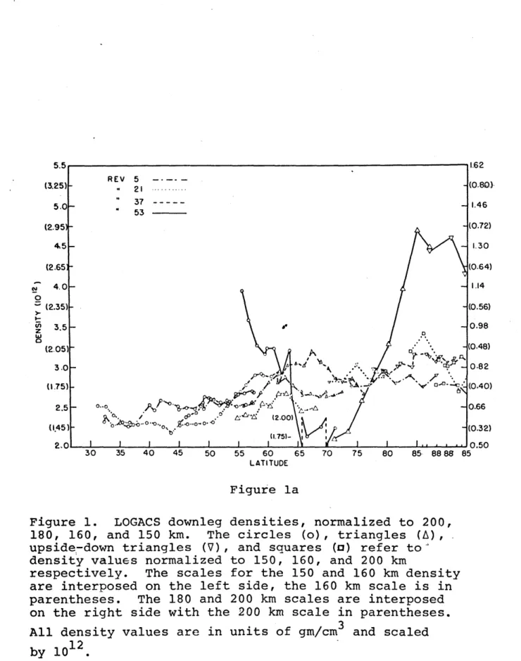
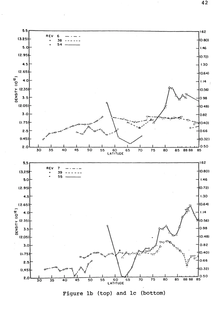
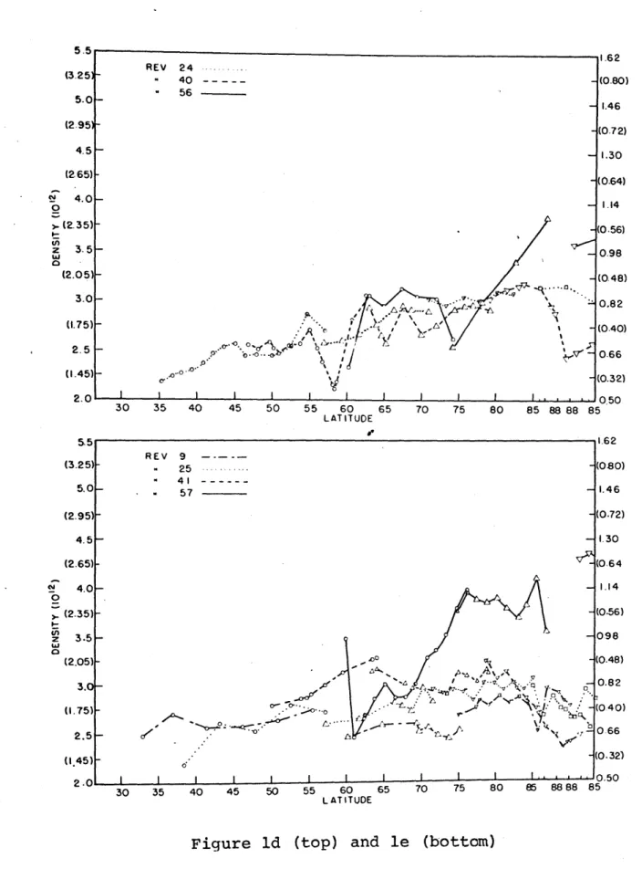
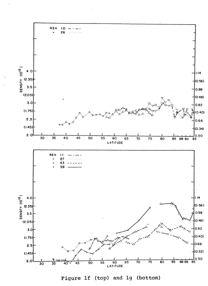
la-o LOGACS downleg densities, normalized to 200,

180, 160, and 150 km. 41-48

2a-o LOGACS densities around Perigee, normalized

to 145 km. 49-56

3a-p LOGACS Upleg densities, normalized to 150,

160, 180, and 200 km. 57-65

4a-j SPADES densities for revs 21-57, normalized

to 160, 180, and 200 km. 68-69

5a-n SPADES densities for revs 157-208, normalized

to 160, 180, and 200 km. 70-72

6a-n SPADES densities for revs 253-292, normalized

to 160, 180, and 200 km. 73-75

7a-o SPADES densities for revs 344-391, normalized

to 160, 180, and 200 km. 76-79

8 Time-geographic latitude analysis of LOGACS

densities converted to 150 km. 93 9 Time-Corrected Geomagnetic latitude analysis

of LOGACS densities converted to 150 km. 94 10 Time-geographic latitude analysis of SPADES

densities converted to 160 km, revs 21-57. 101 11 Time-geographic latitude analysis of SPADES

densities converted to 160 km, revs 157-208. 102 12 Time-geographic latitude analysis of SPADES

densities converted to 160 km, revs 253-292. 103 13 Time-geographic latitude analysis of SPADES

densities converted to 160 km, revs 344-391. 104 14 Time-Corrected Geomagnetic latitude analysis

of SPADES densities converted to 160 km,

revs 21-57. 105

15 Time-Corrected Geomagnetic latitude analysis of SPADES densities converted to 160 km,

6

Figure Page

16 Time-Corrected Geomagnetic latitude analysis of SPADES densities converted to 160 km,

revs 253-292. 107

17 Time-Corrected Geomagnetic latitude analysis of SPADES densities converted to 160 km,

revs 344-391. 108

18 Density variation with longitude, 250S-100 N. 122 19 Density variation with longitude, 100N-450 N. 123 20 Density variation with longitude, 45°N-850N. 125

LIST OF TABLES

Table Page

1 LOGACS Ephemeris data. 16-17

2 SPADES Ephemeris data. 21-22

3 Planetary geomagnetic indices and 2800 MHz solar radio flux observed during the flight of

LOGACS, May 1967. 31

4 Planetary geomagnetic indices and 2800 MHz solar radio flux observed during the flight of

SPADES, July-August 1968. 32

5 Extract from the normalization table for the

150 km standard altitude. 35

6 Conversion factors for reducing standard altitude

densities to a single altitude. 85

7 Qp indices for SPADES. 91

8 Zonal means of LOGACS density data converted to

150 km. 97

9 Zonal means of SPADES density converted to 160 km,

geographic latitude. 110

10 Zonal means of SPADES density data converted to

160 km, Corrected Geomagnetic (C.G.) latitude. 111 11 Seasonal density variation at 160 km. 116

I. INTRODUCTION

Artificial earth satellites have opened up an en-tirely new area of the atmosphere to direct observation. Satellites have proven to be a valuable platform from which the weather and structure of the troposphere and stratos-phere can be observed. A number of scientific satellites have been designed and flown to gather information on the charged particle population and the structure of the geo-magnetic field as well as their interaction with the solar wind. Satellite systems have been launched to provide com-munication and navigation links, to investigate the shape of the geoid and its gravitational field, to find and moni-tor earth resources, and to put men himself as an observer in a new environment. More recently scientific satellites have been orbited to investigate the composition, ionization levels, and atmospheric density of the satellite environ-ment.

The fact that a portion of the atmosphere, however tenuous, is present at the altitudes where satellites are flown causes perturbations and decay of satellite orbits which can be measured and used to infer the atmospheric den-sity near the perigee altitudes of the satellites. By this means a considerable amount of information has been gathered from a large number of satellites on the density structure and variation of the upper atmosphere.

has several very important limitations. The first is that the atmosphere perturbation drag force is not limited to a single point in the atmosphere but extends over a 200 arc or more of the satellite orbit, depending on the orbital

eccen-tricity. Further, the perturbation force is quite small compared to the total orbit energy and due to tracking ac-curacy limitations several revolutions around the orbit may be required before the atmospheric density signal can be adequately isolated. The number of revolutions required is mainly dependent on the minimum altitude of the orbit and the

satellite area to mass ratio. A minimum of two revolutions are required to determine the density. The number actually used is almost always greater, ranging up to several days duration. The resulting density value is thus derived from the integrated atmospheric drag force on the satellite over a range of altitudes down to the minimum altitude, along a 200 arc or more of the orbit for usually six or more revolu-tions around the orbit. Thus the structure and time varia-tions of the density are considerably smeared by the orbital decay observation technique.

The orbital decay density observations are not uni-formly distributed. Relatively few are available from low altitudes due to the more rapid orbit decay rate which quick-ly reduces orbital lifetime. Most satellites with long

design lifetimes are placed in orbits with minimum altitudes above 200-250 km. A further deficiency in the distribution of observations is the lack of high latitude observations.

10

The reason for this is that lack of sufficient rocket

booster capability made it necessary to use a large portion of the earth's angular momentum to put a payload into orbit, thus resulting in relatively low orbital inclinations. More recently more satellites have been launched into near polar orbits but sampling of the high latitude region is still relatively sparse, particularly at certain local times of day at lower altitudes.

Orbital decay observations accumulated for over 10 years have revealed much about the structure and variation of the density in the region of the atmosphere known as the thermosphere. The density in this region is largely con-trolled by solar extreme ultraviolet (EUV) and corpuscular radiations. The density varies over the eleven year solar cycle in concert with the variation of the mean background

solar EUV flux. Shorter term density variations are observ-ed with the appearance and fluctuations of active areas on the solar disk. These result in short-term variations in the solar EUV output which in turn cause density changes with a lag of about one day. The most prominent density variation is that caused by direct solar heating. This

causes a density bulge to form which is thought to be at the latitude of the solar subpoint with a maximum lagging local noon by two hours. Minimum density lags the antisolar point by about 3-4 hours. This subsolar density bulge is believed to migrate with the sun. A rather unexpected semi-annual density varitaion is observed with maxima in early

April and late Oct. and minima in mid-Jan. and late July. The extrema in Oct. and July are larger than those in Jan. and April. There is still considerable disagreement as to the cause of this semi-annual variation. The last recog-nized density variation is that due to corpuscular radia-tion. This is usually associated with geomagnetic activity and in general lags the variation in geomagnetic activity by several hours. Due to the short-term nature of geomag-netic storms the exact character of the atmospheric density response is poorly known from orbital decay measurements. Density increases of two orders of magnitude have been

ob-served at some altitudes in response to a strong geomagnetic storm.

Because of the wide range in the altitude, latitude, local time of day, solar EUV flux level, etc., a model con-cept is used to incorporate the density observations. The model is based on the static diffusion equilibrium equations with a temperature profile specified by the angle from the

center of the modelled sub-solar bulge and the levels of EUV flux and geomagentic activity. Lower boundary

condi-tions of temperature and composition are assumed at a level near 100 km where static diffusion begins to become effect-ive. These lower boundary conditions are based on the

results of various rocket flights. The shape of the temp-erature profile is adjusted to match static diffusion den-sities to those observed over the altitude range up to 1200 km (Echo balloon).

Considerable uncertainty still exists as to the density structure at low altitudes. The nature of the very dynamic response of the density level and distribution are poorly known from orbital decay measurements. Recently density observations have become available from very sensi-tive satellite-borne accelerometers flown aboard two satel-lites. These density observations have high resolution in time and space. Their accuracy exceeds that from orbital decay measurements. A few of these measurements have been presented and discussed in the open literature (DeVries, 1972, 1972b; Forbes and Marcos, 1973; Marcos and Champion, 1972; Marcos et al, 1971). However, to date no thorough, integrated investigation has been made using all or even a large portion of this density data. Density observations by accelerometers have been obtained on 36 different days. The major portion of the data is for altitudes below 200 km. During the days when accelerometer density measurements

were obtained, an extremely large geomagnetic storm occurred. These data afford a unique opportunity to not only obtain information on the low altitude density structure of the thermosphere, but to also determine the nature of the

II. SOURCES OF DATA

The density data used in this study were obtained from the direct measure of the atmospheric drag force by satellite-borne accelerometers. The accelerometers were capable of measuring atmospheric drag forces of less than 10-6g. This level of sensitivity was more than sufficient to measure the drag force accurately on the satellites below 250 km.

The drag force is related to the density by

maD = -1/2pV2CDA (1)

where

m = satellite mass

aD = atmospheric drag acceleration p = atmospheric density

V = satellite velocity along the orbit CD = drag coefficient

A = effective satellite cross-sectional area, normal to the velocity vector.

The advantages of this method of density determination over that of observing satellite orbit decay are very sig-nificant. The accelerometer is capable of determining

drag on a nearly instantaneous basis, thus yielding density information with a high degree of resolution in time and space. This is far superior to the resolution obtained by orbit decay measurements.

THE LOW-G ACCELEROMETER CALIBRATION SYSTEM

Data from two separate satellites are used in this study. The first is the Low-G Accelerometer Calibration System (LOGACS). LOGACS was flown on a United States Air Force Agena satellite placed in near-polar orbit on 22 May 1967. The orbit inclination was 91.50. The initial peri-gee, apoperi-gee, and latitude of perigee were 148 km, 357 km, and 43.30N. On revolution 18 an orbit adjustment was

per-formed which raised apogee to 407 km and reduced the lati-tude of perigee to 40.70 N. During the portion of the

flight in which useful data was obtained these orbital elements decayed to 141 km, 296 km, and 590N respectively, Minimum satellite altitude decayed from 145.1 km on rev 5 to 137.4 on rev 66. The Agena vehicle was

attitude-stabilized in the plane of the local horizon by intermit-tent firing of gas jets in the attitude control system. A single-axis, electrostatically pulse-rebalanced Bell Miniature Electrostatic Accelerometer (MESA) was used. The MESA was placed on a turntable which could rotate in the plane of the local horizon at two precisely fixed rates or be held fixed in either a fore or aft direction relative to the vertical motion. This permitted in-orbit calibra-tion and scaling of the instrument. Density data were obtained by LOGACS up to 330 km but only that portion of the entire data set below 210 km was used in this study. Details on the orbits, times, and locations of the data are

15

given in Table 1. A full description of the instrumenta-tion, data processing methods, and other pertinent details concerning LOGACS are given by Fotou (1968).

A major problem in processing the LOGACS data was the elimination of "noise" from the thrusters of the

vehicle attitude control system. This prevented continuous measurement of the drag force. Other data losses occurred due to tape recorder saturation and to instrument shut-down

during the orbit adjustment period. The data sampling rate was about one observation per second. Final data

resolu-tion time of 20 seconds was obtained from LOGACS. The actual errors in the measured accelerations are estimated to be less than one percent (Bruce, 1968). The absolute density values deduced from the acceleration measurements have a total uncertainty of ±10% due principally to a lack

of knowledge on the precise value of the drag coefficient (Cook, 1965).

A possibly greater source of error is that caused by winds. During the latter portion of the LOGACS flight a major geomagnetic storm occurred. Side-force accelera-tions, normal to the plane of the orbit, were fortuitously obtained during the rotating modes of the MESA. Feess

(1968) made a thorough study of these side forces and the attitude control jet firings necessary to correct for them. The Agena center of mass was different from the sidewards

TABLE 1

LOGACS EPHEMERIS DATA

Inclination, 91.50 Rev No. 5 6 7 9 10 11 12 13 14 18 20 21 24 25 26 27 28 29 30 31 32 33 34 35 36 37 38 39 40 Date GMT 23 May 0203 " 0332 " 0501 " 0759 " 0928 1057 1226 1355 1524 2122 24 May 0020 " 0150 0620 0750 0920 1050 1219 ', 1349 1519 1648 1818 1947 2117 2246 25 May 0015 " 0145 t" 0314 f" 0444 f" 0'613 Minimum Alt. (km) 145.1 145.1 145.1 145.0 144.8 144.7 144.5 144.2 144.2 144.7 144.9 144.8 144.7 144.7 144.6 144.5 144.3 144.2 144.0 144.1 144.0 144.3 144.2 143.9 143.7 143.5 143.5 143.5 143.3 Longitude of the Descending Node(E) Latitude of Min. Alt. 31.00N 31.9 32.4 32.7 33.1 33.5 33.8 34.1 34.4 31.1 31.4 31.8 33.2 33.6 33.8 34.0 34.2 34.4 34.6 34.9 35.1 35.3 35.6 35.9 36.2 36.5 36.7 37.0 37.2 Local Solar Time Declination 126 104 81 37 352 330 307 285 262 195 150 128 60 38 16 354 331 309 286 264 241 219 197 174 151 129 106 84 61 1037 ,1037 1037 1037 1037 1037 1037 1037 1037 1037 1035 1034 1034 1034 1034 1033 1033 1033 1033 1033 1032 1032 1032 1032 1031 1031 1031 1031 1031 20.3 If 11 1 U1 20.4 It If 20.5 11 If it it It 20.6 It If I it If If 20.7 II I It 1" "1 "1

TABLE 1 Continued Rev No. 41 43 44 45 46 47 48 49 50 51 52 53 54 55 56 57 58 59 61 62 63 64 65 66 Date GMT 25 May 0742 " 1040 1210 1339 1508 1637 1806 1935 2105 2234 26 May 0003 " 0132 f" 0301 " 0430 0559 0728 0857 1026 1321 -1552 1620 1849 1918 " 2146 Minimum Alt. (km) 143.3 142.9 142.9 143.0 143.0 143.0 142.9 142.7 142.3 142.0 141.6 141.0 140.8 140.6 140.2 139.9 140.0 140.3 139.7 138.8 138.4 138.1 137.7 137.4 Longitude of the Descending Node(OE) Latitude of Min. Alt. 37.50N 38.0 38.3 38.6 38.9 39.1 39.4 39.6 39.9 40.1 40.3 40.5 40.8 41.1 41.3 41.6 41.9 42.2 42.4 42.5 42.3 42.2 42.4 42.4 Local Solar Time Declination 39 354 332 310 287 265 243 220 198 176 153 130 108 86 64 41 19 357 335 313 291 268 246 224 1031 1030 1030 1030 1030 1030 1030 1029 1029 1029 1029 1029 1029 1029 1029 1029 1028 1028 1028 1028 1028 1028 1028 1028 20.7 I? I! 'i I! 'I II 'I 11 U' I' lI 'I II 20.8 I' I' 'I I' 'I 11 I, U' 'I "! "l

calculate winds normal to the plane of the orbit. He found wind speeds in excess of 1 km/sec in the polar re-gions during the magnetic storm. Fedder and Banks (1972) made theoretical calculations of polar thermospheric wind generation by convection electric fields. They found that neutral wind speeds approaching 800 m/sec in the antisolar direction and 400 m/sec eastward could be generated within 4 to 5 hours by a steady electric field of 40 mV/m. Using a somewhat different theoretical approach Cole (1971) estimated that west to east wind speeds on the order of 2 km/sec could be generated by an auroral electric field which had been observed to reach 100 mV/m. Wind

observa-tions have been made from rocket releases of trimethyl aluminum trails and grenade clouds between 90 and 200 km at high latitudes at twilight. Westward winds of 500 to 600 m/sec were observed following a strong positive magne-tic bay. Between 120 and 150 km there was a strong cor-relation between the E to W neutral wind and the perturba-tion of the H component of the geomagnetic field during the previous two hours (Rees, 1972).

Hayes and Roble (1971) have calculated north to south winds in mid-latitudes of 400 m/sec at 400 km from observations of the Doppler shift of the 6300A emission. This observation was made at night during an auroral event.

Smith (1968) deduced eastward winds at Kauai, Hawaii of 227 m/sec at 147 km from a vapor trail experiment made

18 hours after the peak of geomagnetic storm. Theoretical calculations of winds generated by the subsolar bulge as specified in thermospheric density models, have been made by several investigators using a variety of assumptions regarding boundary conditions, subsolar density bulge amp-litude and shape, and including ion drag but omitting or including various other terms in the equations of motion (Lindzen, 1966, 1967; Geisler, 1966, 1967; Kohl and King, 1967; Challinor, 1968, 1969 and 1970; Dickinson and Geisler, 1968; Rishbeth, 1972). All of these theoretical models

yield maximum winds on the order of 250 m/sec in the lower thermosphere. Satellite velocity for a nearly circular orbit at 200 km is almost 8 km/sec. From equation (1) a wind component of 1 km/sec along or opposite the satellite direction of motion could cause a deduced density error of about ±27%. This error would be restricted to high lati-tudes at times during geomagnetic storms. The observed density variations from LOGACS during the storm period of 25-26 May 1967 were nearly an order of magnitude greater than 27%. Winds of 250 m/sec in the direction of satellite motion would result in a 6% error in the deduced density. The density variations observed with LOGACS during geomag-netically quiescent periods were considerably in excess of

6%. All LOGACS data were obtained at nearly the same local time in the sunlit hemisphere. The theoretical estimates of winds resulting from the subsolar pressure bulge show

20

them to depend mostly on local time and to a lesser extent on latitude and season. Thus on each revolution LOGACS would experience nearly the same variation of wind due to

a subsolar density bulge if the models of its size and shape are accurate. The absolute density values would therefore be in error by an amount no more than 6% but the relative density variation from one revolution to the next would be much less subject to this source of error. The

same argument can be made regarding the error due to the uncertainty of CD . In conclusion, the relative density variations observed with LOGACS are the result of true

thermospheric density variations.

SPADES

The second source of data used in this study is from the USAF/Aerospace Corp./AFCRL satellite OV1-15 (1968-59A) also known as the Solar Perturbation of Atmospheric Density Experiments Satellite (SPADES). SPADES was launched on 11 July 1968 into a 89.80 inclination orbit with an

initial perigee and apogee of 158 km and 1850 km. A more complete description of SPADES payload and orbital data is given by Champion and Marcos (1969) and by Morse (1970). Times and locations of the SPADES accelerometer data used

in this study are given in Table 2. SPADES was spin stab-ilized with three Bell MESA's mounted as near as possible to the vehicle center of mass, aligned normal to each

TABLE 2

SPADES EPHEMERIS DATA

Inclination, 89.80 Date GMT Minimum Alt. (kn) 21 25 29 33 37 41 45 49 53 57 157 160 163 166 172 175 178 181 187 190 199 202 205 208 253 256 259 262 13 July it If 14 July It Is 23 July If It 24 July It It 25 July It 26 July I 'I 30 July It If It 0828 1527 2226 0525 1224 1922 0220 0918 1617 2315 0450 1002 1513 2024 0646 1157 1708 2219 0841 1352 0523 1033 1543 2053 0219 0728 1238 1747 Latitude of Perigee 159.0 158.7 158.6 157.9 157.8 157.7 157.6 157.3 157.6 157.3 150.4 151.4 151.4 152.3 152.6 152.7 152.7 152.8 1,52.7 152.7 152.8 152.9 153.0 153.3 155.6 156.2 156.3 156.4 Longitude of Perigee (E) 12.3 0S 11.4 10.5 9.7 8.9 7.9 7.1 6.3 5.3 4.50 S 17.20N 17.7 18.4 19.0 20.3 20.9 21.6 22.2 23.5 24.2 26.1 26.8 27.5 28.2 38.1 38.8 39.5 40.3 Rev No. Solar Declination Local Time 1117 1116 1115 1113 1112 1111 1110 1109 1108 1106 1037 1036 1036 1035 1033 1032 1031 1030 1029 1028 1025 1024 1023 1022 1010 1009 1008 1007 42.3 297.3 192.4 87.4 342.5 237.6 132.7 27.9 283.0 178.2 86.9 8.8 290.8 212 .8 56.8 338.8 260.9 182.9 27.1 309.2 75.7 357.9 280.0 202.3 117.6 40.0 332.5 245.1 21.70 21.7 21.7 21.6 21.6 21.5 21.5 21.5 21.4 21.4 20.0 19.9 19.9 19.8 19.8 19.7 19.7 19.6 19.5 19.5 19.3 19.2 19.2 19.1 18.3 18.3 18.2 18.2

TABLE 2 Continued

Rev Date GMT Minimum

No. Alt. (km) Latitude of Perigee Longitude of Perigee (oE) Local Time Solar Declination 265 268 271 274 277 280 283 286 289 292 344 352 355 358 361 364 367 370 373 376 379 382 385 388 391 30 July 31 July If I 1 Aug. It I" "I 5 Aug. 6 Aug. It 7 Aug. oI If 8 Aug. If It I 2256 0405 0914 1422 1931 0040 0549 1057 1606 2115 1553 0349 0857 1404 1911 0018 0525 1032 1538 2044 0151 0558 1204 1711 2217 155.9 155.2 155.8 155.4 155.3 155.8 155.9 155.9 156.2 156.6 157.7 157.8 157.9 158.0 158.3 158.0 158.4 158.8 158.9 159.4 159.3 160.3 159.8 159.5 159.6 40.8 41.4 42.1 42.8 43.4 44.2 44.8 45.5 46.1 46.9 59.1 60.7 61.4 62.1 62.8 63.4 64.1 64.9 65.6 66.4 67.1 67.'8 68.5 69.2 69.9 167.6 90.1 12.7 295.2 217.8 140.5 63.1 345.7 268.3 191.0 267.5 87.8 10.8 293.8 216.8 139.9 63.0 346.1 269.2 192.3 115.5 38.6 321.8 245.0 168.2 1006 1005 1004 1003 1002 1001 1000 0958 0958 0958 0938-0943 0935-0941 0932-0940 0927-0939 0923-0939 0918-0938 0824-0937 0627-0936 0222-0935 2219-0934 0341-0933 2128-0932 2128-0932 2035-0931 2116-0930 18.1 18.1 18.0 18.0 18.0 17.9 17.9 17.8 17.8 17.7 16.9 16.8 16.7 16.6 16.6 16.5 16.4 16.4 16.3 16.2 16.2 16.1 16.0 16.0 15.9

23

other, and along and normal to the nominal vehicle spin axis. The SPADES spin axis was fixed normal to the orbit-al plane. The spin rate was initiorbit-ally 10 rpm. Superim-posed upon this was a precession of the spin axis with a period of 23 secs. One of the two MESAs aligned normal to the spin axis failed on launch. In spite of the spin axis precession, the MESA aligned along the spin axis yielded density data of doubtful value. The remaining MESA perfor-med excellently. Above 250 km the accelerometer signal had a constant component due to the centrifugal acceleration resulting from the vehicle spin. This signal was modulated by the precession of the spin axis. As the satellite alti-tude decreased to below 250 km a second modulation due to atmospheric drag began. This modulation occurred at the satellite spin period and increased in amplitude with in-creasing density. Density values were derived by coupling the accelerometer output to separate information on the vehicle attitude. Numerical filtering techniques were em-ployed to eliminate the accelerometer signal due to vehicle dynamics (spin rate and spin axis precession rate) and

yield density values for those times when the MESA was

aligned most nearly into and away from the satellite direc-tion of modirec-tion. Marcos et al (1972) gives a more complete description of the experiment and data processing. The resulting density values have a time resolution of less than one second and are available approximately every three

seconds. The location of the density measurement is with-in 0.10 latitude and 0.1 km altitude. These limits are within the range of the satellite ephemeris errors. Due to power limitations the accelerometer experiment on SPADES was operated only every three or four revolutions around the orbit. Additionally,power supply problems frequently resulted in the loss of data for periods of several days at a time. Data were available for various periods in the interval between 13 July and 28 Sept. 1968. A complete gap occurred in the data between 8 and 28 Aug. During this time the perigee latitude moved over the pole from the sun-lit to the dark hemisphere. Only the data collected

through 8 Aug. was included in this study in order to limit the amount of processing to tractable proportions and also

since the geographical area and local times covered were similar to that of LOGACS.

The statistical errors in the density values de-rived from the accelerometer output are estimated to be: numerical filtering technique, varies from negligible at perigee to ±2% at 250 km, attitude, ±2%, satellite area, ±2%, and overall, ±4% at perigee to ±6% at 250 km (Marcos et al, 1972). Only data below 210 km was used in this study. Even with this limitation, some errors in the den-sity data due to filtering with slightly inaccurate values for the spin and spin axis precession rates are evident in the final data. These will be pointed out later. An

25

additional source of absolute density error of up to ±10% may exist due to uncertainty about the assumed value of

2.2 for C_D (Cook, 1965). As with LOGACS, the accelerometer derived densities from SPADES are subject to errors due to thermospheric winds. During the period covered by data from SPADES there were no large geomagnetic storms. Thus wind speeds of the order of 1 km/sec would not be expected. The comments made regarding the LOGACS data about wind and drag coefficient errors not affecting the measured relative density variations apply equally to the SPADES data.

III. DATA PROCESSING

The density data from the two sources covered the entire altitude range from 210 km to below 138 km. The variation of density with altitude almost completely

dom-inates the density relationships with other parameters. There are several ways of overcoming this difficulty. One

is to compare the density values with those specified by some standard model of thermospheric density for the same time, location, altitude, and solar/geomagnetic conditions.

Ratios of measured to model (Jacchia, 1971) densities have been calculated for the SPADES data at 5 km altitude inter-vals (Marcos et al, 1972). Such a procedure normalizes out any of the density variations specified (perhaps in-correctly) by the model used. The density ratios obtained are not representative of a single altitude but the entire range of altitudes covered by the data. This method re-quires considerable computational effort to obtain the model densities corresponding to the measured values. In his analysis of the LOGACS data obtained during the geomag-netic storm period on 25-26 May 1967, DeVries (1972) chose the data from rev 41 which occurred at the end of a

geomag-netically quiet interval as the basis for the normalization of the subsequent data obtained during the geomagnetic

storm. The normalization was accomplished by computing the ratios of density values at discrete altitudes to those observed during rev 41. This method was undoubtedly chosen

by DeVries for reasons of expediency in order to obtain a quick, rough picture of the density variation associated with the great geomagnetic storm immediately following rev 41. The primary drawback of this technique is the

"representativeness" of the rev 41 data. The density var-iation on a particular revolution may be a significant

function of the geographic or geomagnetic coordinates

sampled. The altitude profile may also contain variations of this sort. Subsequent revolutions do not sample the density at the same location with respect to the earth and even should the ground track of the satellite be the same

24 hours later, the decay of the orbit and the movement of the perigee location would alter the altitude profile of density sampling and change the location of the profile with respect to surface coordinates.

The procedure finally adopted in this study was to use model density profiles to normalize all density values to the nearest of a set of fixed altitudes as was done by DeVries (1966). In this manner the relative density vari-ation could be more easily seen. The density profiles in the most complete, up-to-date model of thermospheric densi-ty available (Jacchia, 1971) were chosen for this purpose.

In the altitude range covered by the data, the density scale height varies from about 14 km at 138 km to 40 km at 210 km. In order to avoid errors from normaliza-tion over too large a range of altitude, the "standard"

altitudes were more closely spaced at the lower heights where the density scale height was smaller. All data below 150 km were normalized to the standard altitude of 145 km. The only data in this height range were from LOGACS. The major fraction of the densities below 150 km were normal-ized over an altitude range of 5 km or less. It was not until revs 62 through 66 that the minimum vehicle altitude

for LOGACS decayed below 140 km to the lowest sampled alti-tude of 137.7 km on rev 66. Densities for altitudes be-tween 145 and 155 km were normalized to 150 km. A 160 km

standard altitude was chosen for data in the 155 to 170 km height range. Densities obtained between 170 and 190 km and between 190 and 210 km were normalized to 180 and 200 km respectively. Between revs 157 and 208 some density values were obtained from the SPADES accelerometer data at altitudes ranging down to 150.4 km. Since the proportion of such data below 155 km was very small and since the scale height at those altitudes was almost 20 km, all such data were normalized up to the 160 km standard altitude.

In all only 14 density values were normalized to a standard altitude over an interval of more than one half the local density scale height. This minimized the effect of any

errors in the model density scale heights on the normalized density values.

The thermospheric density model (Jacchia, 1971), hereafter referred to as J71, was derived by using the

static diffusion equations to match the composition at 150 km as observed from various rocket flights and the ob-served density as derived from satellite orbital decay measurements at greater altitudes. Static diffusion is assumed to begin at 100 km. The temperature profile for the static diffusion equations assumes a constant lower boundary temperature of 1830K at 90 km. The temperature

increases from 90 km to an inflection point at 125 km and then approaches an exospheric temperature value, TO ,

asymptotically. A detailed mathematical description of the temperature profile and the derived density profile is given by Jacchia (1971). The principal variable in J71 is T.* T is calculated from a knowledge of the solar declin-ation, local time, latitude, the geomagnetic index Kp, and the solar radio flux at 10.7 cm (2800 MHz). These factors account for the T. changes and thus density scale height changes with season, time of day, solar corpuscular energy

flux, and solar EUV energy flux. The 2800 MHz solar radio flux is an indicator of the amount of solar EUV radiation absorbed by the thermosphere (Nicolet, 1963; Neupert et al, 1964). This index is very successful in helping to specify T. and thus thermospheric density (Bourdeau et al, 1964; Knight et al, 1973). Use of J71 as a model for the To

variation does not eliminate the modeled density variations from the normalized density values. The change in the

interval of normalization is introduced into the normalized density values. This effect is very small and well below the "natural" variation of the observed density values. For example, the total change in the amplitude of the

diurnal bulge model of J71 between 200 and 210 km over the range of latitudes and local times sampled by LOGACS is less than 0.5%.

T. was calculated exactly by the method given in J71. The values of the three-hour planetary geomagnetic index, Kp, and the 2800 MHz solar radio flux, F10.7, used

in the calculations are given in Table 3 for the LOGACS data and in Table 4 for the SPADES data. A one day lag was used in applying the F10.7 data. The Kp data were used with a 6.7 hr. lag. These lag times approximate the atmos-pheric response time to changes in these indices and are the ones recommended in J71. There is no variation of

response time with altitude (Roemer, 1971a). The response time of the thermosphere to K enhancements has been found to be significantly less than 6.7 hours at high latitudes

(DeVries, 1972; DeVries et al, 1967; Taeusch et al, 1971a, 1971b; Waldteufel et al, 1972). In a situation of rapidly changing magnetic activity the difference between real and model thermospheric density response could introduce some

error in the normalization procedure. Observations of F₁0.7 are made daily and Kp values are derived every three hours. These values were plotted against time with the

TABLE 3

Planetary Geomagnetic Indices and 2800 MHz Solar Radio Flux Observed During the Flight of LOGACS, May 1967

81 F_{1 0}._{7 10.7 K p} 00-03 03-06 06-09 09-12 12-15 15-18 18-21 21-24 QQ 20 143 Q 21 156 QQ 22 178 23 189 24 196 D 25 205 D 26 213 27 208 139 139 139 139 139 139 139 139 2+ 1+ 1+ 10 1- 10 1+ 2+ 10 10 0+ 10 1- 10 3+ 2+ 2+ 10 1+ _1- 0+ 0+ 0+ 00 1- 2- 10 1+ 10 2- 40 3+ 2- 1+ 2- 2- 2+ 3+ 4+ 2+ 2- 20 10 5+ 8+ 7+ 8- 90 90 9- 7+ 7- 7- 4- 40 5-40 3+ 3+ 2+ 30 2- 4+ 4+ 11+ 6 11- 6 6+ 3 15- 9 19- 11 42+ 130 51- 146 26+ 20 1

Monthly five quiet days (QQ), ten quiet days (Q), and five disturbed days (D).

TABLE 4

Planetary Geomagnetic Indices and 2800 MHz Solar Radio Flux

F F

10.7 10.7

Observed During the Flight of 81 Day Q 12 D 13 D 14 Q 15 16 Q 17 18 19 QQ2 0 21 D 22 23 QQ2 4 25 26 27 28 QQ2 9 30 QQ3 1 QQ 1 QQ 2 3 4 5 6 7 8 161 151 151 143 145 139 131 131 130 129 135 142 148 153 150 142 139 140 134 131 130 130 137 132 132 144 136 138 144 144 144 145 145 145 145 146 146 145 145 145 145 145 145 145 145 145 145 145 145 145 145 145 145 145 144 144 SPADES, July-August 1968 K p 00-03 30 2- 6-2+ 20 1-2+ 1+ 3- 2-40 20 1-1+ 3+ 2-1+ 20 1- 2-30 1+ 3+ 3+ 4+ 03-06 2+ 3- 5-20 20 1.0 30 20 1+ 1- 3-2+ 1-10 2+ 3+ 20 2-1+ 1+ 1-10 40 20 3-40 30 3+ 06-09 1- 2-2+ 1+ 20 10 2-2+ 0+ 10 4-10 1+ 20 30 1- 2-10 20 1+ 10 3+ 2- 1-30 30 4-09-12 10 1-2+ 20 10 1+ 1+ 2+ 0+ 1+ 40 3- 1-1+ 4- 3-1+ 10 10 20 1+ 1+ 20 10 30 30 3+ 1+ 12-15 1+ 0+ 30 10 2-20 3+ 1+ 1-2+ 4+ 3+ 1-30 30 3- 2-1+ 20 10 10 1-2+ 0+ 30 20 30 3-K_P 15-18 2+ 50 2+ 1+ 40 1+ 3+ 2+ 10 30 3-10 30 30 1+ 3-1+ 2+ 1+ 1-10 3+ 0+ 3+ 2+ 20

2-iet days (Q), and five disturbed days

18-21 1+ 60 3+ 2+ 3-2+ 10 1+ 1+ 30 3-1+ 1- 2-3+ 1+ 30 10 30 10 1-20 0+ 3- 4- 2-21-24 10 4-2+ 2-1+ 20 10 30 10 3-20 2- 1- 2-40 1+ 2-10 20 10 1-1+ 1+ 2-3+ 3-2+ 3-13 22-26 14 17- 12-17 16 9- 16-26 20-6 14- 23-19 15- 11-14 12-7 8-20 10+ 20 24 22-21+ A p 7 22 22 6 9 6 10 8 5 9 19 11 3 7 15 11 8 5 7 5 4 4 12 6 12 16 13

recommended time lags after first converting Kp values to exospheric temperature increment by use of Table 2b in Jacchia (1971). Linearly interpolated values were read off for the times of the satellite accelerometer readings. To obtain the T. variation due to location with respect to Jacchia's model of the subsolar heating bulge, values of the solar declination and of the latitude and local time of the density observation were used to linearly

interpo-late the ratio of the local temperature to the global min-imum temperature as found in Table 1 of Jacchia (1971). The global minimum temperature is calculated from a

know-ledge of F10.7 and F10.7 where F10.7 is a three solar

rotation or 81-day average of F1 0.7* The exospheric temp-erature increment due to Kp is added to the local tempera-ture to obtain the value of T . To was calculated for all density observations.

The next problem was the calculation of the coef-ficients for normalization of the observed density values. These coefficients varied with the standard altitude,

height difference of the density observation from the stan-dard altitude, and exospheric temperature. The basic

relation for the normalization of density is

where

p = density

z = altitude of the density value H = local density scale height

The subscript "o" refers to values for the standard alti-tude. The principal difficulty in this facet of the nor-malization procedure is the variation of H with altitude. Over the height range of the observed density data, values for H are given for every 5 km below 160 km and every 10 km above 160 km in Table 6 of J71. A separate set of values is given for each 1000 _{K increment of TC. For a given value}

of TO (10000_{K for example) the values of H were plotted} against height, a smooth curve was drawn through the plot-ted points, and values of H were read off at one kilometer intervals. Additional values of H were then linearly in-terpolated from these at 0.2 km intervals. An example of the resulting interpolated H variation with altitude is given in the first two columns of Table 5. A factor of

02

exp(+ ) was calculated for each value of H. Whether the altitude of the value of H was above or below the standard altitude determined the choice of the sign. For the value

0.1

of H at the standard altitude the factor exp(+ 0 ) was computed for both signs. These values are shown in the third column of Table 5. The values in the third column represent the normalization factor for density over a 0.2 km interval (0.1 km either side of the standard altitude)

TABLE 5

Extract from the Normalization Table for the 150 km Standard Altitude

Alt. (km) 148.6 148.8 149.0 .2 .4 .6 .8 150.0 .2 .4 .6 .8 151.0 .2 .4 H_{1 0 0 00} (km) 17.47 17.54 17.61 17.68 17.75 17.82 17.89 17.96 18.03 18.10 18.17 18.24 18.31 18.38 18.45 ±0.2 exp H 0.98862 0.98866 0.98871 0.98875 0.98880 0.98884 0.98888 0.99445 1.00558 1.01115 1.01111 1.01107 1.01103 1.01098 1.01094 1.01090 Fact. 0.91873 0.92931 0.93997 0.95071 0.96152 0.97242 0.98339 0.99445 1.00558 1.01680 1.02810 1.03948 1.05094 1.06248 1.07410 1.08581 H_{1 0 0 0} (km) 17.80 17.87 17.94 18.01 18.08 18.16 18.23 18.30 18.37 18.44 18.52 18.59 18.66 18.73 18.80 ±0.2 exp H 0.98883 0.98887 0.98891 0.98896 0.98900 0.98905 0.98909 0.99455 1.00548 1.01095 1.01091 1.01086 1.01082 1.01078 1.01074 1.01070 Fact. 0.92017 0.93057 0.94105 0.95160 0.96222 0.97292 0.98370 0.99455 1.00548 1.01649 1.02757 1.03873 1.04996 1.06128 1.07267 1.08414 Alt. (km) 148.5 148.7 148.9 149.1 .3 .5 .7 .5 150.1 .3 .5 .7 .9 151.1 151.3 151.5

centered on height values on the left hand column of Table 5. The successive product of these factors to a given al-titude from the standard alal-titude is given in the fourth column of Table 5. These are the normalization factors

for converting density values at heights given in the right-hand column to the standard altitude of 150 km for an exospheric temperature of 10000K. Similar results for

11000K are also given in Table 5. A complete set of such tables was constructed for each standard altitude covering the height range of densities to be normalized to that al-titude. Normalization factors were calculated for each 1000K increment between 10000K and 14000K (the T range of density data). Normalization factors for the even tenths of a kilometer of altitude were linearly interpolated from those calculated at the odd tenths (see Table 5). Linear interpolation was used to obtain the normalization factor at a T intermediate to the calculated values. A density value of 2.52 x 10-12gm/cm3 measured at 148.5 km and with T = 10560K would be converted as follows:

From Table 5 ₁₀₀₀0_{K 1100}0_K

148.5 Fact = 0.91873 0.92017

Difference = 0.00144

Interpolating for 10560K = x 0.56

Interpolation increment = 0.00081

Add back 10000K factor = +0.91873 Final normalization factor = 0.91954 Times the density at 148.5 km = x 2.52 Density value normalized to 150 km = 2.32 x 10-12gm/cm3

Use of the normalization tables derived in the same manner as the portion shown in Table 5 does not introduce

any error into the normalization data other than that in-herent in J71. The Tc calculations are accurate to within ±20K. The error introduced by an inaccurate T, depends upon the size of the normalization interval. For a 1000K error in To the maximum resulting error in the normaliza-tion factor in the entire set of normalizanormaliza-tion tables is

1.3 percent for a 10 km interval. The normalization fac-tors were checked against the density values in Table 6 of J71. Density values are given in Table 6 of J71 for

the same intervals as the scale height. Hence the normal-ization factor for any 5 or 10 km interval of the table could be multiplied by the density at that level and the resulting "normalized" density could then be checked again-st the table density value. For example the density value at 210 km for TC = 10000 in Table 6 of J71 could be nor-malized to 200 km and compared with the 200 km density value for To = 10000K given in the same table. Such a check was made for all the tables of normalization factors at each standard altitude for all the To values used, and over all possible 5 or 10 km intervals where density values

for confirmation were available. The density values in Table 6 of J71 were given to four significant figures and

in no case was a "normalized" density different from the value at the standard altitude by more than one in the

38

fourth significant figure. This confirms the complete accuracy of the tables of factors constructed for the nor-malization of density values.

The largest uncertainty in the normalization pro-cess is the model used for calculating exospheric tempera-ture, To , at high latitudes and particularly during geo-magnetically disturbed conditions. Orbital decay derived densities from high inclination satellites have shown that the atmospheric response to changes in Kp is enhanced at high latitudes. Jacchia et al (1967) report a 15-20% greater density response to AKp for latitudes above 550N as compared to lower latitudes. At 650 the density re-sponse has been found to be 20% higher than at the equator

(Jacchia, 1970). Marcos et al (1971) also found the

density response to geomagnetic activity to increase from the equator to high latitudes. In a very comprehensive

analysis of orbital decay measurements in the 250-800 km altitude range for over 210 geomagnetic storms the follow-ing relation was obtained by Roemer (1971a):

ATO = R (21.4 sin

jIq

ATO = exospheric heating increment due to Kp Kp = the 0.4 day average of K

p p

= geographic latitude

This result yields an.increase from 1190K to 2260K between 00 and 900 latitude for a K _P of 5. Roemer (1971b) later

39

reported that the maximum response was at 600 to 700 but few data were available at latitudes above 700 to confirm this. Density gauge measurements from Explorer 32 made between 300 and 400 km showed that high latitude density was 20% higher than at low latitudes even on quiet days

and that during geomagnetic disturbances the density be-tween 550 and 650 exceeded that at the equator by a factor of three (Newton and Pelz, 1969). Composition measurements from OGO-6 made at 500 km during a magnetic storm showed a 4000 difference in T at the equator and between 600 and 800 geomagnetic latitude (Taeusch et al, 1971b). Doppler temperatures from the 6300A line of OI observed from OGO-6 before and during a 3 day geomagnetic storm have revealed large irregular temperature increases of 3500K at 275 km in the auroral zone (Blamont and Luton, 1972). Equatorial changes were smooth and much smaller (500K) and mid-lati-tude changes were intermediate (110-1250K). After the

storm there was little latitudinal temperature gradient. Even during extended quiet periods before the storm the

temperatures observed at high latitudes were always great-est. The temperature maximum was found at the geomagnetic poles during a storm and not at the auroral zone (Blamont and Luton, 1972). A 4000K underestimate in T. at a To value of 13000K (geomagnetic storm condition during the latter portion of LOGACS) would result in a density

40

Over the same height interval at lower altitudes the error would be less. Thus the normalization process is

relative-ly unaffected even by a severe underestimate of To at high latitudes during geomagnetic storm conditions.

The above calculation assumed the static diffusion profile of J71. During an intense geomagnetic storm the

assumption of a state of static diffusion equilibrium would not be valid. Further, the altitude profile of

auroral heating might not be the same as that which gave the shape of temperature profile used in J71. However, even with these limitations the maximum error in the nor-malized densities is estimated to be less than 4 percent. Such an error would occur only in those densities normal-ized over a 10 km interval during the peak of the geomag-netic storm that occurred during the latter day and a half of the LOGACS flight. The maximum anticipated error due

to the normalization procedure would be considerably less for the major portion of the density data.

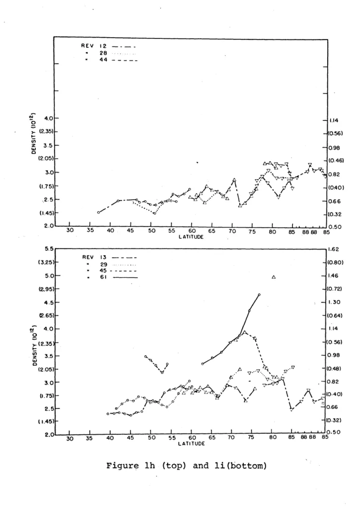
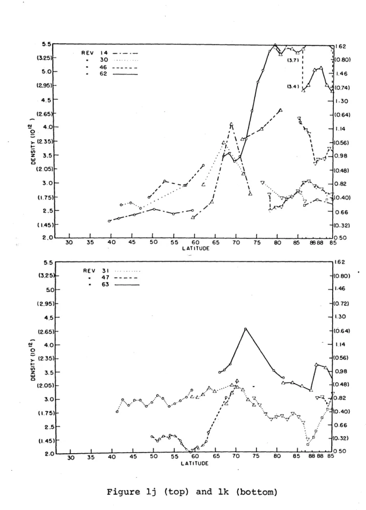
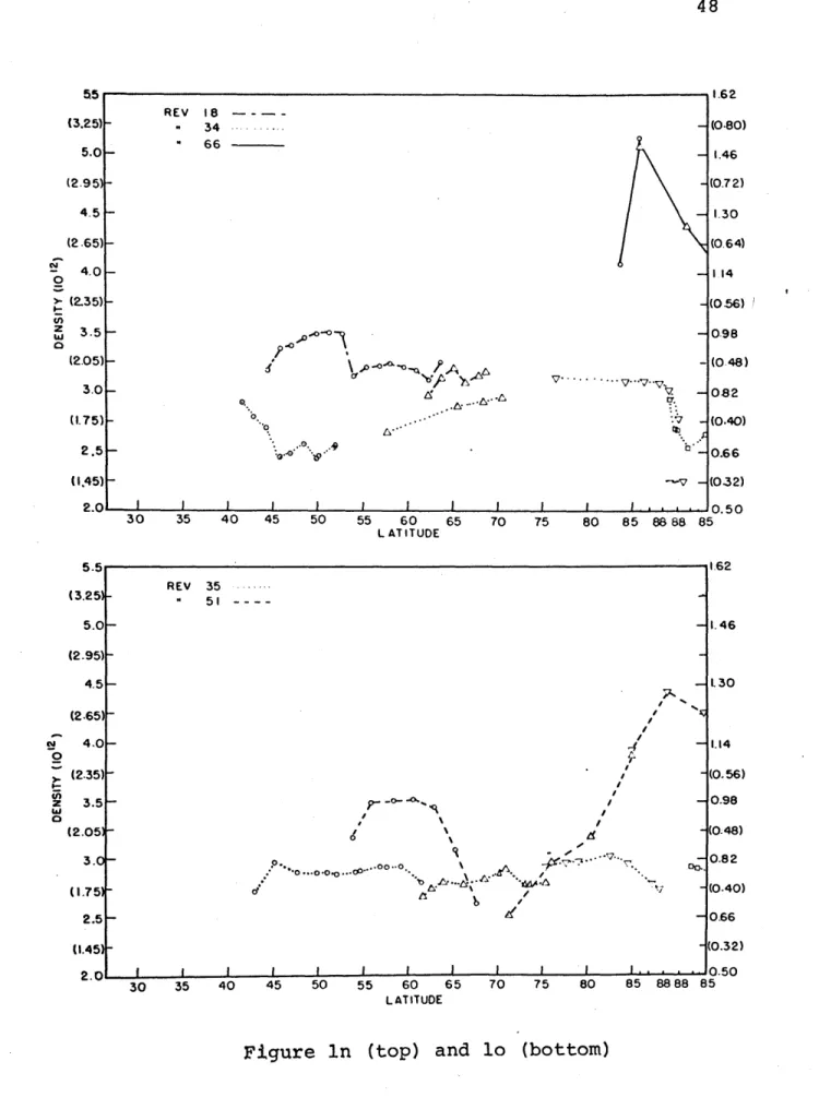
The normalized density values for LOGACS are shown in Figures 1, 2, and 3 plotted against geographic latitude. Densities normalized to 200, 180, 160, and 150 km obtained while the LOGACS vehicle was approaching perigee are dis-played in Figure 1. In Figure 1 circles are used for

den-sity normalized to 150 km, triangles for 160 km, upside down triangles for 180 km, and squares for 200 km. The densities around perigee, normalized to 145 km, are

5 1.6b REV 5 -.. -21 " 37 " 53 0? 4 a ~9." o cP, o ' . .. (2.00) • o. -,to...o, eo..o-o. ( 1.75)-I I I 1 50 55 60 LATITUDE ,Ad 6\dr °"° 65 70 (0.80) 1.46 (0.72) 1.30 (0.64) 1.14 (0.56) 0.98 (0.48) 0.82 (0.40) -0.66 - (0.32) I I.. 0.50 75 80 85 8888 85 Figure la

Figure 1. LOGACS downleg densities, normalized to 200, 180, 160, and 150 km. The circles (o), triangles (A), upside-down triangles (V), and squares (o) refer to-density values normalized to 150, 160, and 200 km

respectively. The scales for the 150 and 160 km density are interposed on the left side, the 160 km scale is in parentheses. The 180 and 200 km scales are interposed on the right side with the 200 km scale in parentheses. All density values are in units of gm/cm3 and scaled

12 by 10 (3.25) (2.95)- (2.651-4.0 (n 3.5 z (2.05) 3.0 (1.75) 2.5 (i.45) Sn 30 35 40 45 -- ---- - - 5.0-

4,5-5.5 (3.25) 5.0 (2.95) 4.5 (2.65) 4.0 (235] 3.5 (2.05) 3.0 (1.751 2.5 (1.45) 2.0 30 35 40 45 50 55 60 65 LATITUDE 1.62 (0.80) 1.46 (0.72) 1.30 (0.64) S1.14 (0.56) 0.98 (0.48) S" 0.82 (0.40) .7 - 0.66 (0.32) 0.50 70 75 80 85 88 88 85

Figure lb (top) and ic (bottom)

a -I I I I I I I I I 30 35 40 45 50 55 60 65 70 LATITUDE REV 6 -- 38 - 54 I I 1.62 (0.80) 1.46 (0 72) 1.30 (0.64) 1.14 (0.56) 0.98 (0.48) 0.82 (0.40) 0.66 (0.32) 0.50 5.5 (3.25) 5.0 (2.95) 4.5 (2.65) 4.0 (2.-35) 3.5 (2.05) 3.0 (1.75) 2.5 (1.45) 2.0 REV 7 -..-- 39 3955---" 55 .0 A i I l I 0-0 1 ---- --- --- - I~ ____ I m 34 0' , P

-43 (3 (2 (2 o -(2 I., z 0 (2. (I (I (3 (2 (2 0 . (2 v-z (2 (I (I 5.5 .251 5.0 .951 4.5 65) 4.0 .35) 3.5 .051 3.0 .75) 2.5 .451 2.0 55 88 85 REV 24 S40 - ( - 40---56 .0 0 _S(C ... c -c e ' . , -( I I I I I I I .. . . .. I62-REV 9 --.25) - 25 . O(8C - 41 5.0 57 1.46 .95)- (0.72 4.5 - 1.30 .65) (0 .6, 4.0- 1.14 .35) (0.56 3.5 -098 .05) -0o -(0.48 3.0 - -a \b~

v

Figure Id (top) and le (bottom)

.62 0.80) 1.46 0.72) 1.30 0.64) 1.14 ).56) ).98 0.48) ).82 .40) ).66 0.32) .50 30 35 40 45 50 55 60 65 70 75 80 85 88 LATITUDE

-- ---

-- ---

REV 10 ----26 P. D. .0 o..** *'~ 0. ... . ... I I I a I i I I I I I I I. . . 30 35 40 45 50 55 60 65 70 75 80 85 88 88 8 LATITUDE REV II ---S 27 ... - 4 3 - 59 1.14 (0.56) 0.98 (0 48) 0.82 (0.40) 0.66 (0.34) 0.50 5 Ja 7 "- \ -. . , _{1--l I} 50 55 60 65 70 75 LATITUDE 30 35 40O 45 80 85 8888 85 1.14 (0.56) 0.98 (0.46) 0.82 (0.40) 0.66 (0.32) 0.50

Figure if (top) and ig (bottom)

4.0 (2.35) 3.5 (205) 3.0 (1.75) 2.5 (1.45) 2.0 4.0 (2.35) 3.5 (2.05) 3.0 (1.75) 2.5 (1.45) 2.0 -- ~- ~~-~~~ --- ---I' 1

-REV 12 ----" 28 " 44 o '* 1 , I I I 1 1 L~rl~1~2 ~7 ~~h-d'~ Vs~ aP a a 30 35 40 45 50 55 60 65 70 75 80 85 LATITUDE 5. 8888 8! REV 13 " 29 ... 45---61

I

Figure lh (top) and li(bottom)

4.0 (2.35) 3.5-(2.05) 3.0 (1.75) (2 .5 (1.45) -. (3.251 5.0 (2.95) 4.5 (2.65) 4.0 0 >. (2.35) z 3.5 (2.05) 3.0 (1.75) 2.5 (1.45) 9. 1.14 (0.56) 0.98 (0.46) 0.82 (040) 0.66 (0.32 0.50 5 1.62 (0.80) 1.46 (0.72) 1.30 (0.64) 1.14 (0.56) 0.98 (0.48) 0.82 (0-40) 0.66 (0.32) 0.50 15 I 5

B

-

---

---- ---

--

__

_~

5-(3.25) 5.0(2.95) -4.5 (2.65) 4.0 (2.35 " 3.5-(2.05) 3.0 (1.75) 2.5 (1.45) 2.0 5.5 (3.25) 50 (2.95) 4.5 (2.65) 4.0 (2.35) 3.5 (2.05) 3.0 (1.75) 2.5 (1.45) 2.0 55 60 LATITUDE 30 35 40 45 50 55 60 65 LATITUDE 65 70 75 /7 dA 80 85 8888 85 1.62 (0.80) 1.46 -(0.72) - 1.30 -(0.64) - 1.14 -(056) 098 (0.48) q. - -0.82 .. 7 0.40) -0.66 .. (0.32) .... 050 75 80 85 88 88 85

Figure lj (top) and ik (bottom)

REV 14 --- 1-30 (3.7) S46 -62 / , 4' I , , I .-I \ " L .I 'I 5, 30 35 40 45 50 REV 3 1 ... - 47 63 .0 .. P . o. o .o' " : "o".o Si . I P .. i,--- i-~~ ~-~~- -- --- -- - --- --- ---p 5. --I I ,I I ' - ~-. -C 162 (0.80) 1.46 (0.74) 1.30 (0.64) 1.14 (0.56) 0.98 (0.48) 0.82 (0.40) 0.66 (0.32) 0 50

47 5.5 (2 (2 o0 (2 (2 (I (I zI 30 35 40 45 50 55 60 65 1 70 LATITUDE 75 80 85 8888 8 REV 32 - 48 . ~.25) 48---56 5.0-.95) 4.5

.o

Figure 11 (top) and Im (bottom)

- --I _1.62 (0.80) 1.46 (0.72) 1.30 (0.64) 1.14 (0.56) 0.98 (0.48) 0.82 (0.40) 0.66 (0.32) 0.50 5

REV 18 - 34 66 5 (3.2! 5. (2.9 4. (2.6 4. (2.3 3. (2.0 3. 2, (1.4 2. 5. (3.2 5 (2.9 4 (2.6 4, (2.3 3, (2.0 3 (1.7 2. (1.4 2. 5 5) 0 5) 5 5) 0 5) 5) 0 5) .5 5) .0 .5 -v SI I I I I I I I I I .. 30 35 40 45 50 55 60 65 70 75 LATITUDE ''0 .4 .. 9 80 85 8888 REV 35 " 51--.0 - I 5) 5) -5) R .5 ,o- -1 (C So I I I I I I 1 . S. "o...o-o.o..ao''' ' ''° '- . 5 8 8 85 .5 - O 5) C n f i l I I , I I I I . 30 35 40 45 50 55 60 65 70 75 80 LATITUDE

Figure In (top) and lo (bottom)

1.62 .46 30 .14 0.56) ).98 ).48) ).82 ).40) .66 ).32) ).50 \ p-0 /' f n . .- ' b 85 8888 85 - - --- --- -- -- ---1.62 -(0.80) - 1.46 (0.72) 1.30 (0.64) - 114 -(056) -0.98 - (0.48) - 082 -(0.40) -0.66 -(032) - 0.50 85 = i I I I I I I I I . . . . * I v

5.5 -(6.5 50 -(6.0 4%5- 4.0-3.5 3.0

2.51

Figure 2. LOGACS densities around perigee, normalized to 145 km. The density values have the units of gm/cm3 and are scaled by 1012

49 5 21 .. . 37 53.-REV ) ) 70 75 ~L~b~Qt~H;e" --- ---6-11

50 5.51-5. O0 N 4.5 z w o 4.0 3.5 -3 .0-10 15 20 25 30 35 40 45 50 55 60 65 70 75 LATITUDE .0 REV 7 - -39 - - -o 55 0.. p-0% '1 O b -0 -. , 2.51 I I I I I I I I I I I I 10 15 20 25 30 35 40 45 50 55 60 65 70 75 LATITUDE

Figure 2b (top) and 2c (bottom)

REV 6 38 54 -o 0* .. o '--O1 o ' - ... o.. 0I0 I I I I I I I 1 ' I l l4b N z _4.0 4.0 5. %- 3.5-

3.01-5. 5. 0 4. I-z w 4. 3 3. 9 REV 24 40 S56 5- 0-5 0-I P 0 -0. . .o-' I I I I I I I I I I I I I I0 15 20 25 30 35 40 45 LATITUDE REV 9 I 25 5.5- 5.0-c,1 0 4.5- t-(n z 0 4.0 3.5-S 41 ---S57 -od r, C 00~ ... 0..~ .4 . _* , , ° ., 0 " " "" -*. -n. 00 0' '0*0 -.0zo 10 15 20 25 30 35 40 45 50 55 60 65 70 75 LATITUDE

Figure 2d (top) and 2e (bottom) Nor-'

15 20 25 30 35 40 45

LATITUDE

50 55 60 65 70 75

(top) and 2g (bottom) 6.01 5.5 5.0 4.5- 4.0- 3.5- 3.0-2. REV 26 o o * o 0 . . 0o O 0.. O . . I I I I I I I I 10 Figure 2f ~--- --- --- --- - --__ , Ii .-r5

6.0 5.5 5.0-o S4.5 U) z 4 4.0 2.51 I I I I I I I I I I I I I 10 15 20 25 30 35 40 45 LATITUDE 5.51-5.0 o 0 4.5 >- I-z 4.0- 3.51-50 55 60 65 70 75 REV 13 * 29... 45 " 61 p-o 0.. P ₉ t' % 'I r "o0

A

a,'o

Figure 2h (top) and 2i (bottom)

REV 1 2 - 28 * ~~*~= -~~~i- -- ~ -~~; :;;-: i- ~--- -: --~-~"-~ - ~~~-~-- --- I I

P-~

C;, REV 14 30 " 46 - 62

js

b

Figure 2j (top) and 2k (bottom)

5.0-0 4.5 -cn z 4. 4.0 3 .5- 3.0-0 4.5 i-cn z 4.0 3.51-3.0

8r