Secondary maxima in ozone profiles

(1)

HAL Id: hal-00301170

https://hal.archives-ouvertes.fr/hal-00301170

Submitted on 23 Mar 2004

HAL is a multi-disciplinary open access

archive for the deposit and dissemination of sci-entific research documents, whether they are pub-lished or not. The documents may come from teaching and research institutions in France or abroad, or from public or private research centers.

L’archive ouverte pluridisciplinaire HAL, est destinée au dépôt et à la diffusion de documents scientifiques de niveau recherche, publiés ou non, émanant des établissements d’enseignement et de recherche français ou étrangers, des laboratoires publics ou privés.

Secondary maxima in ozone profiles

R. Lemoine

To cite this version:

R. Lemoine. Secondary maxima in ozone profiles. Atmospheric Chemistry and Physics Discussions, European Geosciences Union, 2004, 4 (2), pp.1791-1816. �hal-00301170�

(2)

ACPD

4, 1791–1816, 2004 Secondary maxima in ozone profiles R. Lemoine Title Page Abstract Introduction Conclusions References Tables Figures J I J I Back Close

Full Screen / Esc

Print Version

Interactive Discussion

Atmos. Chem. Phys. Discuss., 4, 1791–1816, 2004 www.atmos-chem-phys.org/acpd/4/1791/

SRef-ID: 1680-7375/acpd/2004-4-1791 © European Geosciences Union 2004

Atmospheric Chemistry and Physics Discussions

Secondary maxima in ozone profiles

R. Lemoine

Royal Meteorological Institute of Belgium

Received: 9 January 2004 – Accepted: 3 March 2004 – Published: 23 March 2004 Correspondence to: R. Lemoine (rene.lemoine@meteo.be)

(3)

ACPD

Full Screen / Esc

Print Version

Ozone profiles from balloon soundings as well as SAGE II ozone profiles were used to detect anomalous large ozone concentrations of ozone in the lower stratosphere. These secondary ozone maxima are found to be the result of differential advection of ozone-poor and ozone-rich air associated with Rossby wave breaking events. The fre-5

quency and intensity of secondary ozone maxima and their geographical distribution is presented. The occurrence and amplitude of ozone secondary maxima is related to ozone trends in the total ozone column and in the lower stratosphere ozone concentra-tion at Uccle and can be used as a measure of the influence of atmospheric circulaconcentra-tion on the ozone distribution at mid-latitudes.

10

1. Introduction

Laminated ozone structures in the lower stratosphere have long been observed in ozone vertical profiles. Laminae observed in ozone vertical profiles from ozoneson-des, are local extrema of the ozone concentration, situated in the lowermost part of the stratosphere. A lamina can be a local maximum or minimum of the concentration with 15

a limited vertical extent of typically a few hundreds of meters. In some circumstances several laminae can be observed in one profile. In this case, layers of ozone-poor and ozone-rich air alternate. A secondary ozone maximum is the extreme case of a lam-ina where the maximum in the lower stratosphere is the same order of magnitude as the mid-stratospheric ozone concentration maximum. The associated minimum is well 20

pronounced with concentrations well below the average.

Laminae in ozone profiles are very common at mid latitudes and have been the sub-ject of many studies discussed below. Some studies consider laminae and secondary maxima in ozone vertical profiles separately while others do not. The border line be-tween laminae and secondary maxima can only be chosen arbitrarily, as all amplitudes 25

(4)

ACPD

Full Screen / Esc

Print Version

secondary maximum.

Different approaches seem to coexist in the literature. The first, introduced by

Dob-son (1973) suggests that laminae are created through stratosphere-troposphere ex-change near the subtropical jet stream. This view was shared byVarsotos et al.(1994) who analyzed a set of 29 soundings performed above Athens and found a significant 5

correlation between the appearance of laminar events and the establishment of a north-northwest circulation over the site in the lower stratosphere and when the site is under influence of polar air. They present their results as more evidence of the enhancement of laminar phenomena at the vortex boundary. The authors came to the conclusion that what they called ozone minima (laminae with a large vertical extent) occur when 10

the site is under the influence of the subtropical jet stream, showing that ozone minima are associated with air coming from the subtropics.

The second view (Reid and Vaughan,1991) presents differential advection of air from different locations as the likely origin for laminae. But as this process is most active at high latitudes in winter and spring, the authors rule out the suggestion made byDobson

15

(1973) that laminae originate near the subtropical jet stream. Instead, the authors suggested that folds beneath the polar night jet might form laminae near the edge of the polar vortex. Although the possibility remains that a small number of laminae may be generated by stratosphere-troposphere exchange, Reid and Vaughan suggested that laminae may represent evidence of a process that can cause exchange of air in 20

and out of the polar vortex.

Reid and Vaughan(1991) and Reid and Vaughan (1993) define ozone laminae as

features between 200 m and 2.5 km in vertical extent which form a distinct layer of magnitude greater than 20 mPa. They separated genuine laminar structure from large scale features considered as maxima, and treated them separately. They found that 25

laminae are most commonly found between 12 and 18 km at high latitudes in winter and spring. The abundance and amplitude of laminae increase with increasing latitude and the thickness decreases with increasing latitude. Laminae were found to have a typical thickness of 1.5 km and an amplitude of 35 mPa. For the origin of laminae, they

(5)

ACPD

Full Screen / Esc

Print Version

suggested that a mechanism operates at the lower edge of the polar vortex (where ozone mixing ratio increases sharply on isentropic surfaces) which transports ozone to middle latitude in the form of laminae, particularly during spring when the polar vortex dissipates. Possible candidates for this mechanism are inertia-gravity waves associated with the subtropical jet stream as proposed byDanielsen et al. (1991) or 5

distortions of the polar vortex boundary by synoptic scale motions as proposed byTuck

et al. (1992).

Reid et al.(1994), using the EASOE ozonesonde archive, analyzed the occurrence of laminae in the course of the 1992 winter confirming the findings ofReid and Vaughan

(1991) and Reid and Vaughan (1993). Laminae are most abundant near the edge of 10

the polar vortex and are generally absent above 430 K inside the vortex. Observation of inertia-gravity waves in the lower stratosphere appears to suggest that such waves are not of sufficiently large amplitude to cause the kind of laminae that are observed.

Yet another approach to this phenomena is to use Lagrangian techniques to study laminated features in the ozone field. Plumb et al. (1994) and Waugh et al. (1994) 15

used Lagrangian techniques to study the behavior of trace constituents in the boundary of the lower stratospheric vortex. Plumb et al. (1994) showed that vortex intrusions also occur during strong ridging events, during which the vortex is disrupted by one or several large-scale ridges. Such intrusions can lead to the formation of elongated thin filaments of mid-latitude air inside the vortex.

20

Orsolini(1995) andOrsolini et al.(1997) used model simulation to demonstrate that trace species laminae appear in a model as a consequence of isentropic advection in the presence of a vertical shear. Such isentropic advection leads to filamentation of a tracer distribution which has gradients near the vortex edge. Sheets with high tracer content are eroded from the polar vortex and vertically tilted in the vicinity of the polar 25

jet. During strong events, sheets with low tracer content also intrude into the vortex. Sloping or strongly deformed sheets appear as laminae in tracer vertical profiles.

Appenzeller et al. (1997) determined regions in the middle atmosphere where the abundance of ozone laminae or laminae in a tracer distributed as potential vorticity

(6)

ACPD

Full Screen / Esc

Print Version

(PV) is expected to be high. They estimated that laminae generation is expected to be most efficient where vertical wind shears coexist with tracer horizontal gradients. They based their calculation on the size of the thermal wind shears derived from satel-lite temperature observations, and the size of ozone/tracer horizontal gradients. They showed that the production rate of ozone laminae has a dip between 30 and 10 hPa, 5

likely because of the reversal of the ozone latitudinal gradient, and it then maximizes near 5 hPa.

In contrast with most of the above mentioned articles, this paper concentrates on laminae of larger vertical extent, often referred to as secondary ozone maxima. This paper is organised as follows. Section2presents the data used in this study. Section3

10

gives the definition of a secondary ozone maximum and two examples are given in Sect. 4. The relation between the occurrence of ozone secondary maxima and the atmospheric circulation is developed in Sect.5. Sections 6and7present an in-depth analysis of ozone secondary maxima observed in ozone soundings at Uccle (Belgium) and in SAGE II ozone profiles. Section8 describes the possible link between ozone 15

trends and the occurrence of ozone secondary maxima.

2. Dataset description

Ozone soundings have been performed at Uccle, Belgium, since 1969 three times a week with two main interruptions in 1985 and 1986. Brewer-Mast ozone sensors were used from the beginning until March 1997 when it was decided to use model Z ECC 20

ozone sensors. The vertical resolution of an ozone sounding is better than a few 100 meters. Given the high vertical resolution, ozonesondes are the most suitable instru-ment to study laminated structures in the lower stratosphere. A complete comparison between Uccle ozone profiles and SAGE II ozone profiles was performed byLemoine

and De Backer (2001). 25

The Stratospheric Aerosol and Gas Experiment II (SAGE II) is a seven-channel sun spectrophotometer launched in October 1984 aboard the NOAA ERBS satellite. SAGE

(7)

ACPD

Full Screen / Esc

Print Version

uses the solar occultation technique that measures the attenuation of the solar radia-tion by the Earth’s atmosphere at the limb due to scattering and absorpradia-tion by different atmospheric species, primarily at 600 nm (Mc Cormick, 1987). During each space-craft sunrise and sunset SAGE II provides water vapour, ozone, nitrogen dioxide and aerosol extinction profiles. The resolution of the instrument is not homogeneous, with 5

a horizontal extent of the measurement of 200 km along the line of sight and 2.5 km in the perpendicular direction. The vertical resolution is set to 0.5 km in data version 6.0 and profiles extend from the tropopause up to 60 km altitude.

We used geopotential height, potential vorticity maps and wind fields to analyse the synoptic weather situation for a number of case studies. These data were provided by 10

the European Center for Medium-range Weather Forecast.

3. Definition of an ozone secondary maximum

In this study, we only consider ozone secondary maxima. We define an ozone scondary maximum as a layer of ozone-rich air where the ozone partial pressure is at least 75% of the ozone pertial pressure at the main maximum and that is separated 15

from the main maximum by a layer of ozone-poor air where the ozone partial pressure is at most 75% that of the secondary maximum. There are no upper or lower limits on the thickness of the ozone-poor and ozone-rich layers. In order to be used in this survey, the ozone sounding must have reached the 20 hPa level to ensure that the main ozone maximum was measured. The same criteria are applied to SAGE II profiles to 20

detect secondary maxima. The lower vertical resolution of the SAGE profiles should have little or no influence on the detection of secondary maxima: given the usually observed thickness of the ozone-rich and ozone-poor layers (see Sect.4), secondary ozone maxima are resolved by SAGE.

(8)

ACPD

Full Screen / Esc

Print Version

4. Examples

Two examples of secondary ozone maxima measured at Uccle on 12 April 2000 and 19 April 2002 are shown in Fig.1. The measured ozone partial pressure was converted to number density to allow easy comparison with zonal-mean ozone profiles computed with SAGE II data for the same month for the period 1984–2000. The comparison 5

shows that, according to the altitude, different parts of the measured ozone profile compare with average profiles of different latitude bands. The secondary maxima, situ-ated around 12 km altitude in both cases, show extremely large ozone concentrations, amounting to more than two standard deviations above the 40–50◦N SAGE mean (Uc-cle is located 50.8◦N). The associated minimum in ozone concentration around 15 km 10

shows ozone concentrations similar to those observed at much lower latitudes. The air sampled above 20 km shows ozone concentrations that are typical for high-latitude air-masses in the example of 2000 and for mid-latitude air in the example of 2002.

5. Secondary ozone maxima and Rossby wave breaking

In the northern hemisphere, planetary-scale Rossby waves constitute a primary source 15

of dynamical variability. Given the long chemical lifetime of ozone in the lower strato-sphere, reversible transport associated with Rossby waves accounts for the largest part of ozone variability in winter and spring. In addition to reversible transport, irreversible transport occurs during Rossby wave breaking events. Such events are associated with troposphere-stratosphere exchange and tropopause folds. Wave breaking events 20

can be classified as either “equatorward” or “poleward”. On potential vorticity maps, equatorward breaking events, tongues of high potential vorticity (PV) air extend equa-torward and in poleward events, tongues of low PV air extend poleward.

Peters and Waugh (1996) studied a number of Rossy-wave-breaking events which

resulted in the poleward advection of upper tropospheric air from the subtropics dur-25

(9)

ACPD

Full Screen / Esc

Print Version

intruded tropospheric air tilts upstream, thins and is advected cyclonically and type 2 (P2) in which the air tilts downstream, broadens and wraps up anticyclonically. P1 breakings are expected on the cyclonic side of jets and P2 on the anticyclonic side. The authors observed that Rossby waves propagate along the jet and break in the region of weak zonal winds. They also noted that the wave breaking events occurred in two 5

preferred locations that are consistent with the preferred regions of blocking: Atlantic Ocean/Europe and Pacific Ocean/North America.

P2-type wave-breaking events can lead to the advection of air from close to the sub-tropical jet stream into the mid-latitude lower stratosphere. This mechanism can lead to the formation of ozone secondary maxima, as was shown byO’Connor et al.(1999). In 10

the two case-studies presented in that paper, breaking events led to irreversible trans-port of air from the subtropics to the mid-latitudes, up to 365K potential temperature.

P1 and P2-type wave breaking events seem to be the most common origin of ozone secondary maxima observed at Uccle. We used PV maps on 315 K and 330 K potential temperature levels from the ECMWF assimilation system to analyse the synoptic situ-15

ation on days when a secondary ozone maximum was observed at Uccle. Out of 17 well-resolved secondary ozone maxima events observed between January and April in 2001 and 2002, 7 were associated with P1 wave breaking events, 7 with P2 events and 3 could not be easily classified or were associated with equatorward wave breaking events. In all cases where a P1 or P2 event was identified, Uccle was situated on the 20

Eastern or Northern edge of the poleward intrusion, but outside it and under a trough of low geopotential height and high PV air at 315 K that preceded the intrusion. The lower stratospheric ozone-rich air layer was associated with high PV values above Uccle, and could be best observed at 315 or 330 K potential temperature levels. On the other hand, PV fields at the height of the ozone-poor air layer above Uccle (about 100 hPa or 25

430 K) were generally completely different with no signature of the equatorward wave structure.

Five detailed cases studies of ozone secondary maxima events have been per-formed. These events took place in 2000, 2001 and 2002. In addition to the above

(10)

men-ACPD

Full Screen / Esc

Print Version

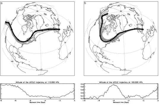
tioned synoptic situation analysis, we used ECMWF wind field analyses to compute 10 days backward isentropic trajectories with the FLEXTRA trajectory model (Stohl,2001, and references therein). Clusters of trajectories were used to check the reliability of the result. Trajectories were started at the height of the secondary maxima and associated minima. An example is given in Fig.2.

5

The results obtained are summarised Table1. In all cases, the low ozone content air masses that make the ozone minima were advected from 30–40◦N latitude across the Atlantic up to western Europe. The overall vertical displacement of these air parcels is descending with an initial altitude between 14 km and 18.5 km at −10 days. The amplitude of the vertical displacement along the trajectory can be as large as 2.5 km 10

in several cases. It is important to note here that even if Rossby wave breaking events have been identified as the likely origin of stratosphere-troposphere exchanges (Peters

and Waugh,1996) that play a role in the appearance of mini ozone holes (Hood et al.,

1999). The results obtained here rule out the possibility that the ozone-poor air layer observed with ozone secondary maxima is air of tropospheric origin. The ozone-poor 15

air mass has its origin the the lower stratosphere and is advected downward along the isentropes.

The ozone-rich air masses are of polar origin and are associated with high (vortex-like) PV values at the same altitude in the ECMWF PV maps. The corresponding back trajectories pass generally North of 70◦N latitude within 10 days before the secondary 20

maximum was observed at Uccle. There is no pronounced systematic vertical positive or negative displacement and the vertical displacement amplitudes are smaller than 1.5 km.

6. Frequency and seasonal cycle

Uccle ozone soundings were systematically scanned for secondary maxima and we 25

calculated the relative frequency of occurrence (RF) of secondary ozone maxima, that is, the fraction of ozone soundings at Uccle that showed a secondary ozone maximum.

(11)

ACPD

Full Screen / Esc

Print Version

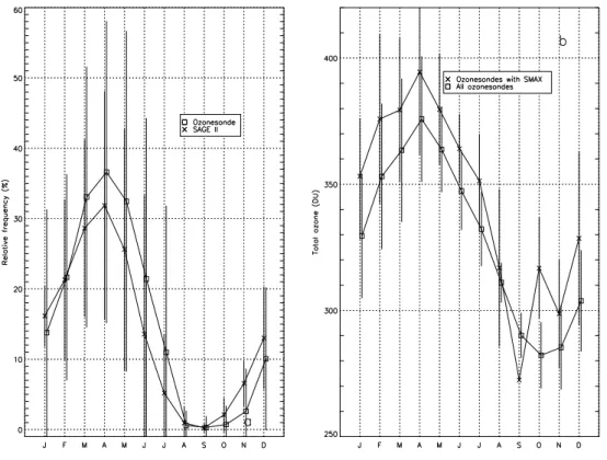
Figure 3a shows the monthly mean RF averaged over the period 1969–2001. Sec-ondary maxima RF are higher during winter with a maximum in March–May. The RF decrease sharply in June and July and fall to almost zero from August to November. This figure is consistent with the scenario where laminae and secondary maxima ap-pear in conjunction with intense planetary wave activity and large disruptions of the 5

polar vortex. The maximum RF occurs in March–April (Fig.3a), which is the time of the year when the final breakdown of the northern polar vortex generally occurs.

As the occurrence of secondary maxima is closely related to the state and position of the polar vortex, the occurrence of secondary maxima should also show some cor-relation with the total ozone column. It is clear from Fig. 3b that secondary maxima 10

RF are highly correlated with the total ozone seasonal cycle at Uccle. Figure3b also shows that the total ozone column is, in the average, higher than the climatology by 20 DU when a secondary maximum is observed. This can be explained by the fact that the tropopause is generally lower in or near the polar vortex than outside of it. And indeed, the observed average tropopause altitude for secondary ozone maxima 15

events (Fig.4a) is lower than the average tropopause altitude for all soundings by 1 to 2 km. It is interesting to note that there is almost no seasonal cycle in the tropopause height when a secondary ozone maximum is observed while there is one in the mean tropopause height. Total ozone columns are higher even if the ozone minimum repre-sents a loss compared to an undisturbed typical vortex ozone profile. The integrated 20

ozone value between the tropopause and the minimum (Fig.4d) varies between 40 and 80 DU with large case-to-case variations.

The criterion to select secondary maxima uses relative differences between the sec-ondary maximum and main maximum and between the minimum and secsec-ondary max-imum. Hence, there is no truncation at some threshold level and it makes sense to 25

look at the absolute ozone concentration of the secondary maxima and its associated minima. Values are shown in Fig.4b. The ozone partial pressure at the secondary maximum has a well pronounced seasonal cycle while the partial pressure of the min-imum shows little variation over the year. The cycle of the secondary maxmin-imum partial

(12)

ACPD

Full Screen / Esc

Print Version

pressure corresponds to the seasonal cycle of the lower stratospheric polar ozone, as ozone accumulates at the base of the polar vortex during winter, see Sect. 5. The partial pressure of the minimum is representative of lower stratospheric low latitude air which undergoes little seasonal variation. It is also clear from this figure that sec-ondary maxima are more pronounced (larger ozone concentration difference between 5

the minimum and the maximum) between December and April than the rest of the year. Ozone secondary maxima at Uccle occur typically around 140 to 160 hPa in winter and spring and below the 170 hPa level in summer (see Fig.4c). This seasonal cycle is less pronounced in the corresponding curve of the associated minima. The minima typically occur around the 90 to 100 hPa level in winter and spring, with somewhat lower 10

altitudes in summer. In this case, the larger pressure difference between the minimum and the maximum occurs in summer and is smallest in October and November.

7. Zonal distribution

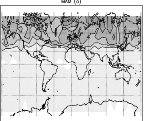
Using SAGE II ozone profiles, the zonal mean RF as well as the longitude/latitude dis-tribution of secondary ozone maxima can be investigated in much more detail than 15

in previous studies. Of particular interest is the longitude/latitude distribution shown in Fig.5. The most striking features are the strong differences between the two hemi-spheres and the latitude gradient of the RF, with no ozone secondary maxima observed in the tropics and highest RF at high latitudes.

Ozone secondary maxima are not evenly distributes in longitude, as expected 20

from the observed association between secondary maxima and Rossby wave activ-ity (Sect.5). In the Northern hemisphere, secondary maxima appear preferentially in regions and at times where the atmospheric circulation is active, and planetary wave activity perturbs the polar vortex. Furthermore, the maximum RF in the north-eastern Atlantic, North Sea and Denmark seems to correspond to the eastern side of the north-25

ern Atlantic storm track (e.g.James,1994).

(13)

mea-ACPD

Full Screen / Esc

Print Version

sured in the ozone hole show low ozone values in the mid stratosphere, much like a secondary maximum. It is therefore very difficult to separate profiles showing a real dynamical secondary maximum, from ozone hole-type profiles where low ozone val-ues in the lower stratosphere are due to chemical depletion, at least at high latitudes. Nonetheless, it is clear that ozone secondary maxima occur much less frequently in 5

the SH mid latitudes, (where no interference with the ozone hole is possible) than in the NH mid latitudes.

8. Trends in atmospheric circulation and ozone variation

8.1. Trends in secondary maxima

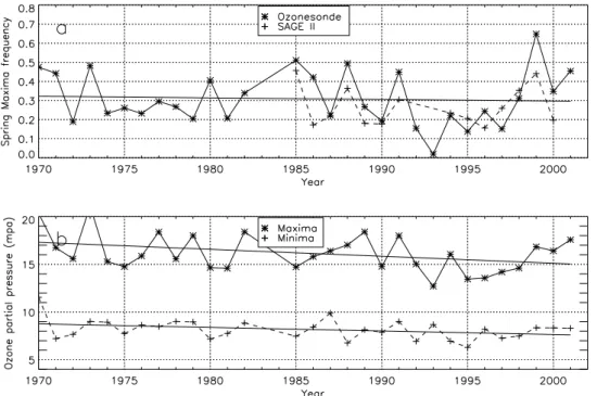
Figure6a shows the time series of the mean Feb-May secondary maxima RF observed 10

in Uccle ozone soundings and SAGE II profiles between 45◦N and 55◦N latitude. Large year to year variations can be observed in both time series but with a reasonable correlation between Uccle and SAGE II even if SAGE II data are zonal mean values.

Figure 6b shows the mean Feb-May intensities of the ozone concentration of the secondary maxima and minima. Both show large year to year variations. A linear 15

regression on the time series shows a significant negative trend for the secondary maximum intensity of −4.5%±2.2% per decade (1σ), similar to the −5% per decade trend at 200 hPa at Resolute (75◦N) for the period 1970–1996 (WMO,1998).

Hood et al. (1999) and Steinbrecht et al. (2001) used one or several parameteri-zations of the atmospheric circulation in order to evaluate the contribution of the at-20

mospheric circulation to decadal ozone trend in winter and spring month. In a similar exercise, followingFusco and Salby(1999) who showed that inter annual variation of total ozone operate coherently with variations of planetary wave activity, it could be tried to use the RF of observed secondary ozone maxima as a measure of the plan-etary wave activity at a given location. We tried to relate this RF to the fluctuation of 25

(14)

sec-ACPD

Full Screen / Esc

Print Version

ondary maxima at a given station is representative of the frequency of maxima on a global scale. Although the zonal distribution is inhomogeneous (see Fig.5), the RF of secondary maxima observed at Uccle compare reasonably well with the zonal mean values calculated from by SAGE II (see Figs.3and 6a).

The second parameter that can also be used to describe the atmospheric ozone 5

content variability is the intensity of the secondary maxima. This value can be taken as a measure of the lower polar vortex ozone concentration and can be expected to have an influence on the average lower stratospheric ozone content as well as total ozone content down to mid latitudes. This is supported by the fact that most of the day-to day ozone variability comes from ozone variations in the lower stratosphere. It 10

is important to note that any long term trend in ozone concentration due to chemical ozone depletion in the lower polar vortex could influence the intensity of secondary maxima.

8.2. Trends in ozone

A simple multiple linear regression model was used to describe both the average total 15

ozone content in spring above Uccle and the average ozone concentration in the lower stratosphere in spring above Uccle.

The ozone variability is described by

O₃(t)= C₀t+ C₁SMAX_{F req}(t)+ C₂SMAX_{Intensi ty}(t)+ C₃SF (t) (1) where O₃(t) is the ozone time series, C₀is the fitted decadal trend, SMAX_{F req}(t) is the 20

ozone secondary maxima relative frequency, SMAX_{Intensi ty}(t) is the ozone secondary maxima intensity time series, and SF (t) is the solar flux variability.

This linear regression model was applied on the 30 years long time series of total ozone and lower stratospheric ozone concentration at Uccle. The total ozone time-series is the mean total ozone column measured at Uccle by the Dobson instrument. 25

(15)

ACPD

Full Screen / Esc

Print Version

The linear regression presented here includes a linear trend, the RF, and the intensity of ozone secondary maxima measured at Uccle and the solar flux variability. This model is not intended to provide a complete description of the contributions to ozone variations. However, this model that simulates a simple linear trend and the influence of two dynamical parameters is able to account for 73% of the average spring (February to 5

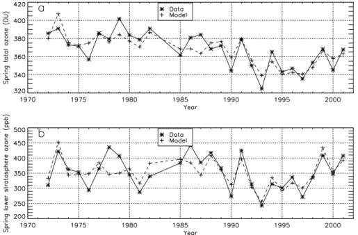
April) total ozone variability. The correlation coefficient between the time series and the regression model is R=0.86. The same model is able to account for 63% (R=0.79) of the lower stratospheric ozone concentration variability. The lower stratospheric ozone is taken to be the average ozone concentration between 11 and 13 km altitude. The results are shown in Fig.7.

10

Looking at the spring lower stratospheric ozone concentration first (Fig.7b), we see that the model is able to reproduce a large part of the variability. The long term trend calculated with the model is −1.68%±2.38% per decade (1 sigma uncertainties). This value is not significant, even at the 68% confidence level. This figure can be compared to the value of −2.44% per decade obtained with a simple linear regression. This 15

means that the ozone variability and the observed long term ozone trend in the lower-most stratosphere can be described with the dynamical index given by SMAX_{F req} and a measurement of the lower polar vortex ozone concentration given by SMAX_{Intensi ty}. Since there is almost no long term trend in the RF time series (Fig.6a), this means that the trend in the lower stratospheric ozone concentration at Uccle is explained by trend 20

in the polar lower stratosphere ozone content, represented here by SMAX_{Intensi ty}. The spring total ozone column variability (Fig. 7a), on the other hand, cannot be described by the parameterization alone as the remaining trend given by the regres-sion model is is −3.26%±0.67% per decade and is 2σ-significant. This trend can be explained by ozone depletion in the mid and upper stratosphere, at altitudes above 25

those where ozone secondary maxima appear. Ozone depletion at mid-latitudes mea-sured by ozonesondes shows significant negative trends that maximizes in the pres-sure range 200–50 hPa (WMO,2002), thus extending well above typical altitudes of the phenomena studied here. Therefore, the trends in the middle and upper-stratosphere

(16)

ACPD

Full Screen / Esc

Print Version

are not accounted for by the parameterization used here. The remaining trend of −3.26%±0.67% is representative of the total ozone trend that is directly due to the effective reduction of ozone concentration in the middle atmosphere at mid latitudes.

9. Conclusions

Thirty years of ozone soundings at Uccle and 15 years of SAGE II ozone profile data 5

were analyzed to look for strong lamination events in the lower stratosphere called ozone secondary maxima.

This study showed that:

– Ozone secondary maxima observed in ozone soundings at Uccle occur

system-atically in conjunction with Rossby wave breaking events, mostly poleward back-10

ward and forward wave breaking events.

– Ozone secondary maxima are most frequent in spring in both datasets and show

a seasonal cycle that follows closely the total ozone seasonal cycle. Using SAGE II ozone profiles, the zonal distribution of secondary maxima can be ob-served. This zonal distribution is not homogeneous, with a correlation between 15

the places of occurrence of ozone secondary maxima and atmospheric circulation patterns.

– Using trajectory calculations, we found that secondary ozone maxima are

cre-ated through differential advection in the lower stratosphere of ozone-rich air that comes from Northern high latitudes underneath ozone-poor air advected from 20

close to the tropics. Ozone secondary maxima are probably not the result of stratosphere-troposphere exchange as suggested byDobson(1973).

– Year-to year variation of the mean relative frequency of ozone secondary maxima

as well as the variation of the mean intensity of the maxima can be used as an easily accessible measure of the atmospheric dynamical activity, or at least its 25

(17)

ACPD

Full Screen / Esc

Print Version

component that has a direct influence on atmospheric ozone content variability. A multiple linear regression model using these two quantities can explain 73% of the mean February–April total ozone variability with a remaining trend of −3.26% per decade. The same model applied on the lower stratospheric ozone content explains 63% of the variability with no significant remaining trend.

5

Acknowledgements. This work was supported by the EUMETSAT Ozone Satellite Application Facility program. SAGE II ozone data are made available on-line by the NASA Langley Research Center (NASA-LaRC) and the NASA Langley Radiation and Aerosols Branch. The FLEXTRA trajectory model is made available by A. Stohl, Technical University of Munich. 10

Edited by: M. Dameris

References

Appenzeller, C. and Holton, J. R.: Tracer lamination in the stratosphere: a global climatology, J. Geophys. Res., 102, 13 555–13 569, 1997. 1794

Danielsen, E., Hipskind, R. S., Starr, W., Vedder, J., Gaines, S., Kley, D., and Kelly, K.: Ir-15

reversible transport in the stratosphere by internal waves of short vertical wavelengths, J. Geophys. Res., 96, 17 433–17 452, 1991. 1794

Dobson, G. M. B.: The laminated structure of the ozone in the atmosphere, Q. J. R. Meteorol. Soc., 99, 599–607, 1973. 1793,1805

Fusco, A. and Salby, M.: Interannual variations of total ozone and their relationship to variations 20

of planetary wave activity, J. Climate, 12, 1619–1629, 1999. 1802

Hood, L., Rossi, S., and Beulen, M.: Trend in lower stratospheric zonal winds, Rossby wave breaking behavior, and column ozone at northern midlatitudes, J. Geophys. Res., 104, D20, 24 321–24 339, 1999. 1799,1802

James, I. N.: An introduction to circulating atmospheres, Cambridge University Press, 1994. 25

1801

Lemoine, R. and De Backer, H.: Assesment of the Uccle ozone time series quality using SAGE II data, J. Geophys. Res., 106, 14 515–14 523, 2001. 1795

(18)

ACPD

Full Screen / Esc

Print Version

Manney, G. L., Bird, J. C., Donovan, D. P., Duck, T. J., Whiteway, J. A., Pal, S. R., and Car-swell, A. I.: Modeling ozone laminae in ground-based Arctic winter time observations using trajectory calculations and satellite data, J. Geophys. Res., 103, 5797–5814, 1998.

McCormick, M. P.: SAGE II: An overview, Adv. Space Res., 7, 3, 219–226, 1987. 1796

O’Connor, F. M., Vaughan, G., and De Backer, H.: Observation of subtropical air in the Euro-5

pean mid-latitude lower stratosphere, Q. J. R. Meteorol. Soc., 125, 2965–2986, 1999. 1798

Orsolini, Y. J.: On the formation of ozone laminae at the edge of the Arctic polar vortex, Q. J. Royal Meteorol. Soc., 528, 1923–1941, 1995. 1794

Orsolini, Y. J., Hansen, G., Hoppe, U.-P., Manney, G. L., and Fricke, K. H.: Dynamical modeling of wintertimelidar observations in the Arctic: ozone laminae and ozone depletion, Q. J. R. 10

Meteorol. Soc., 123, 785–800, 1997. 1794

Orsolini, Y. J., Manney, G. L., Engel, A., Olvarez, J., Claud, C., and Coy, L.: Layering in strato-spheric profiles of long-lived species: Balloon-borne observations and modeling, J. Geophys. Res., 103, 5815–5825, 1998.

Peters, D. and Waugh, D. W.: Influence of barotropic shear in the poleward advection of upper-15

tropospheric air, J. Atmos. Sci., 53, 21, 3013–3031, 1996. 1797,1799

Plumb, R. A., Waugh, D. W., Atkinson, R. J., Newman, P. A., Lait, L. R., Schoeberl, M. R., Browell, E. V., Simmons, S. J., and Loewenstein, M.: Intrusions into the lower stratospheric Arctic polar vortex during the winter of 1991/1992, J. Geophys. Res., 94, 11 437–11 448, 1994. 1794

20

Reid, S. J. and Vaughan, G.: Lamination in ozone profiles in the lower stratosphere, Q. J. R. Meteorol. Soc., 117, 825–844, 1991. 1793,1794

Reid, S. J., and Vaughan, G.: Ozone laminae near the edge of the stratospheric polar vortex, J. Geophys. Res., 98, 8883–8890, 1993. 1793,1794

Reid, S. J., Vaughan, G., Mitchell, N. J., Prichard, I. T., Smit, J. H., Jorgensen, T. S., Varot-25

sos, C., and De Backer, H.: Distribution of ozone laminae during EASOE and the possible influence of inertia-gravity waves, J. Geophys. Res., 21, 1479–1482, 1994. 1794

Steinbrecht, W., Claude, H., K ¨ohler, U., and Winkler, P.: Interannual changes of total ozone and northern hemisphere circulation patterns, J. Geophys. Res., 28, 7, 1191–1194, 2001. 1802

Stohl, A.: A 1-year Lagrangian “climatology” of airstreams in the Northern Hemisphere tropo-30

sphere and lowermost stratosphere, J. Geophys. Res., 106, 7263–7279, 2001. 1799

Tuck, A. F., Davies, T., Hovde, S. J., Noguer-Alba, M., Fahey, D. W., Kawa, S. R., Kelly, K. K., Murpy, D. M., Proffitt, M. H., Margitan, J. J., Loewenstein, M., Podolske, J. R., Strahan, S. E.,

(19)

ACPD

Full Screen / Esc

Print Version

and Chan, K. R.: PSC-processed air and potential vorticity in the northern hemisphere lower stratosphere at mid-latitudes during winter, J. Geophys. Res., 97, 7883–7904, 1992. 1794

Varotsos, C., Kalabokas, P., and Chonopoulos, G.: Association of the laminated vertical ozone structure with the lower stratospheric circulation, J. Appl. Meteorol, 33, 473–476, 1994. 1793

Waugh, D. W., Plumb, R. A., Atkinson, R. J., Schoeberl, M. R., Lait, L. R., Newman, P. A., 5

Loewenstein, M., Toohey, D. W., and Webster, C. R.: Transport out of the lower stratospheric Arctic vortex by Rossby Wave breaking, J. Geophys. Res., 99, 1071–1088, 1994. 1794

World Meteorological Organization (WMO): SAPRC/IOC/GAW Report No. 1, Assessment of trends in the vertical distribution of ozone, Ozone Research and Monitoring Project Report No. 43, 1998. 1802

10

World Meteorological Organization (WMO): Scientific assessment of Ozone Depletion: 2002, Global Ozone Research and Monitoring Project Report No. 47, 2002. 1804

(20)

ACPD

Full Screen / Esc

Print Version

Table 1. Altitudes and latitudes of the back trajectories calculated for the ozone-rich (MAX) and ozone-poor (MIN) air-masses observed with a secondary ozone maximum. All trajectories end above Uccle (50.8◦N, 4.35◦E.)

Date Airmass Origin of the Altitude Altitude airmass at −10 days (km) above Uccle (km) 20000407 MAX 61.3◦N at -6 days 11.5 11.8 MIN 36.7◦N at -9.5 days 13.8 13.5 20000412 MAX 85.7◦N at -6.6 days 12.3 11.3 MIN 29.7◦N at -10 days 18.3 16.6 20010226 MAX 77.3◦N at -9.5 days 13.8 14.6 MIN 39.6◦N at -8.1 days 16.7 15.7 20010330 MAX 71◦N at -10 days 12.3 12.7 MIN 34.5◦N at -10 days 15.9 15.2 20020419 MAX 78.3◦N at -7.7 days 12.7 13.0 MIN 34◦N at -10 days 17.7 16.0

(21)

ACPD

Full Screen / Esc

Print Version

Figures

Fig. 1. Example of ozone secondary maxima observed in ozone soundings on April 12, 2000 (left) and April 19, 2002

at Uccle (right). For comparison, SAGE II mean ozone profiles are shown for 30-40◦N (dot-dashed curve), 40-50◦N (dashed curve) and 60-70◦N (dotted curve). The grey curve is the air temperature.

Fig. 2. 10 days isentropic back trajectory clusters and altitude of the trajectory starting above Uccle. Clusters are

made of 25 trajectories with starting points on a 2 by 2 degree grid centered on Uccle and spaced by 0.5 degree. (a) trajectories starting at 110hPa on 20010330 12h00UT. (b) trajectories starting at 160hPa on 20010330 12h00UT. The pressure levels correspond to the pressure at which the secondary ozone maximum and minimum were observed in the sounding

Fig. 1. Example of ozone secondary maxima observed in ozone soundings on 12 April 2000 (left) and 19 April 2002 at Uccle (right). For comparison, SAGE II mean ozone profiles are shown for 30–40◦N (dot-dashed curve), 40–50◦N (dashed curve) and 60–70◦N (dotted curve). The grey curve is the air temperature.

(22)

ACPD

Full Screen / Esc

Print Version

Fig. 1. Example of ozone secondary maxima observed in ozone soundings on April 12, 2000 (left) and April 19, 2002

at Uccle (right). For comparison, SAGE II mean ozone profiles are shown for 30-40◦N (dot-dashed curve), 40-50◦N (dashed curve) and 60-70◦N (dotted curve). The grey curve is the air temperature.

Fig. 2. 10 days isentropic back trajectory clusters and altitude of the trajectory starting above Uccle. Clusters are

made of 25 trajectories with starting points on a 2 by 2 degree grid centered on Uccle and spaced by 0.5 degree. (a) trajectories starting at 110hPa on 20010330 12h00UT. (b) trajectories starting at 160hPa on 20010330 12h00UT. The pressure levels correspond to the pressure at which the secondary ozone maximum and minimum were observed in the sounding

Fig. 2. 10 days isentropic back trajectory clusters and altitude of the trajectory starting above Uccle. Clusters are made of 25 trajectories with starting points on a 2 by 2◦ grid centered on Uccle and spaced by 0.5◦.(a) Trajectories starting at 110 hPa on 30 March 2001, 12:00 UT. (b) Trajectories starting at 160 hPa on 30 March 2001, 12:00 UT. The pressure levels correspond to the pressure at which the secondary ozone maximum and minimum were observed in the sounding.

(23)

ACPD

Full Screen / Esc

Print Version

Fig. 3. (a) Secondary maxima monthly mean relative frequencies in Uccle ozone soundings and SAGE II ozone profiles

in the latitude band 45-55N. (b) Total ozone column above Uccle for days with a secondary maximum and for all days with a sounding.

Fig. 3. (a) Secondary maxima monthly mean relative frequencies in Uccle ozone soundings and SAGE II ozone profiles in the latitude band 45–55◦N.(b) Total ozone column above Uccle for days with a secondary maximum and for all days with a sounding.

(24)

ACPD

Full Screen / Esc

Print Version

Fig. 4. (a) Monthly mean tropopause altitude for soundings with a secondary maximum and for all soundings. (b)

Monthly mean ozone partial pressure of the secondary maxima and of the associated minima. (c) Monthly mean air pressure at the level of secondary maxima and associated minima. (d) Integrated ozone between the tropopause and the minimum concentration height. This graph gives the mean total ozone content of the secondary maximum. Error bars are one standard deviation on the mean. The period covered is 1969-2001.

Fig. 4. (a) Monthly mean tropopause altitude for soundings with a secondary maximum and for all soundings. (b) Monthly mean ozone partial pressure of the secondary maxima and of the associated minima.(c) Monthly mean air pressure at the level of secondary maxima and asso-ciated minima. (d) Integrated ozone between the tropopause and the minimum concentration height. This graph gives the mean total ozone content of the secondary maximum. Error bars are one standard deviation on the mean. The period covered is 1969–2001.

(25)

ACPD

Full Screen / Esc

Print Version

Fig. 5. Mean distributions of the percentage occurrence of ozone secondary maxima relative frequencies computed

from SAGE II ozone profiles for (a) March to May and (b) September to November. Areas where no data are available are white.

Fig. 6. (a): mean secondary maxima relative frequency in spring, from ozonesonde and SAGE II data. (b): mean ozone

partial pressure of the ozone secondary maxima and minima, from ozonesonde data.

Fig. 5. Mean distributions of the percentage occurrence of ozone secondary maxima relative frequencies computed from SAGE II ozone profiles for(a) March to May and (b) September to November. Areas where no data are available are white.

(26)

ACPD

Full Screen / Esc

Print Version

from SAGE II ozone profiles for (a) March to May and (b) September to November. Areas where no data are available are white.

Fig. 6. (a): mean secondary maxima relative frequency in spring, from ozonesonde and SAGE II data. (b): mean ozone

partial pressure of the ozone secondary maxima and minima, from ozonesonde data.

Fig. 6. (a) Mean secondary maxima relative frequency in spring, from ozonesonde and SAGE II data. (b) Mean ozone partial pressure of the ozone secondary maxima and minima, from ozonesonde data.

(27)

ACPD

Full Screen / Esc

Print Version

Fig. 7. (a): mean spring Dobson total ozone at Uccle and results of the linear regression model. (b): mean lower

stratospheric spring ozone content at Uccle and result of the linear regression model.

Fig. 7. (a) Mean spring Dobson total ozone at Uccle and results of the linear regression model. (b) Mean lower stratospheric spring ozone content at Uccle and result of the linear regression model.