HAL Id: hal-00298326
https://hal.archives-ouvertes.fr/hal-00298326
Submitted on 26 Mar 2007
HAL is a multi-disciplinary open access
archive for the deposit and dissemination of
sci-entific research documents, whether they are
pub-lished or not. The documents may come from
teaching and research institutions in France or
abroad, or from public or private research centers.
L’archive ouverte pluridisciplinaire HAL, est
destinée au dépôt et à la diffusion de documents
scientifiques de niveau recherche, publiés ou non,
émanant des établissements d’enseignement et de
recherche français ou étrangers, des laboratoires
publics ou privés.
Isabel near landfall
F. M. Bingham
To cite this version:
F. M. Bingham. Physical response of the coastal ocean to Hurricane Isabel near landfall. Ocean
Science, European Geosciences Union, 2007, 3 (1), pp.159-171. �hal-00298326�
www.ocean-sci.net/3/159/2007/
© Author(s) 2007. This work is licensed under a Creative Commons License.
Ocean Science
Physical response of the coastal ocean to Hurricane Isabel near
landfall
F. M. Bingham
Center for Marine Science, Univ. of North Carolina Wilmington, 5600 Marvin K. Moss Lane, Wilmington, NC 28409, USA Received: 8 June 2006 – Published in Ocean Sci. Discuss.: 17 October 2006
Revised: 27 February 2007 – Accepted: 14 March 2007 – Published: 26 March 2007
Abstract. Hurricane Isabel made landfall near Drum
In-let, North Carolina on 18 September 2003. In nearby On-slow Bay an array of 5 moorings captured the response of the coastal ocean to the passage of the storm by measur-ing currents, surface waves, bottom pressure, temperature and salinity. Temperatures across the continental shelf de-creased by 1–3◦C, consistent with a surface heat flux
esti-mate of 750 W/m2. Salinity decreased at most mooring loca-tions. A calculation at one of the moorings estimates rainfall of 11 cm and a net addition of fresh water at the surface of 8 cm. The low-pass current field shows a shelf-wide move-ment of water, first to the southwest, with an abrupt reversal to the northeast along the shelf after landfall. Close analysis of this reversal shows it to be a disturbance propagating off-shore at a speed somewhat less than the local shallow water wave speed. The high-pass current field at one of the moor-ings shows a significant increase in kinetic energy at periods between 10 min and 2 h during the approach of the storm. This high-pass flow is isotropic and has a short (<5 m) ver-tical decorrelation scale. It appears to be closely associated with the winds, Finally we examined the surface wave field at one of the moorings. It shows the swell energy peaking well before the wind waves. At the height of the storm, as the winds rotated rapidly in the cyclonic sense, the wind wave direction rotated as well, with a lag of 45–90◦.
1 Introduction
The ocean’s response to the passage of a hurricane has been studied extensively in stratified, deep water environments (e.g. Price, 1981, 1983; Shay and Ellsberry, 1987; Withee and Johnson, 1988; Ginis and Sutyrin, 1995; Shay and Chang, 1997; Jacob et al., 2000). The issues that have been
Correspondence to: F. M. Bingham
most important in these studies are the often-observed right-ward bias in the ocean as a result of coupling between the wind vector’s rotation and inertial motion (Shay et al., 1989; Price et al., 1994), a wake of cool, upwelled water, and the dominance of the response in the near-inertial band (Geisler, 1970).
By contrast, comparatively little work on ocean responses to hurricane forcing has been carried out in shallow waters (e.g. Chu et al., 2000). The complicating factors affecting hurricane response in shallow water include nearby coastal boundaries, potential lack of stratification, bottom stress, rapidly changing topography and the proximity of western or eastern boundary currents (Xie et al., 1998). Chu et al. (2000) reporting on the passage of tropical cyclone Ernie through the South China Sea found many of the same phenomena ex-pected in deep water, rightward bias, near-inertial flows, and strong SST cooling. However, their study was mainly mod-eling, and used little real data from coastal areas. Hurricanes in coastal areas vary greatly in their size, shape, wind distri-bution, wind speed, translation speed and angle of approach towards the coast. All of these factors can potentially af-fect the way the ocean responds to the impulsive and rapidly changing winds.
There have been a few previous studies of the effects of hurricanes on continental shelf environments (Williams et al., 2001; Keen and Glenn, 1999; Keen and Allen, 2000; Smith, 1978, 1982; Murray, 1970; Kohut et al., 2006). Smith (1982) examined currents and temperature on the Florida in-ner and mid-shelf after Hurricane David in 1979. He found a strong transient response in the currents at both locations and cooling of almost 10◦C at the mid-shelf. The cooling was
at-tributed to upwelling and advection. The current response was a mainly along shore. Some response was also noted in the across-shelf direction, but was described as deflected along-shelf flow. Smith’s study involved only two widely separated study locations. The mid-shelf location was highly stratified before, during and after the storm.
22
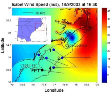
Fig. 1. Wind speed at 16:30 on 18 September 2003. Color bar at
right gives scale in m/s. Winds obtained from the Hurricane Re-search Division. Note the eye of the storm passing over Drum Inlet, NC. Also shown are the locations of the 5 CORMP moorings, OB1, OB2, OB3, OB4 and OB27 (Table 1), and Frying Pan Tower (FPT). At each mooring location and at FPT, wind vectors are displayed showing the modeled direction and speed, with winds generally blowing towards the east or southeast. A scale for the wind vec-tors is shown at the upper left along with an inset map showing the location of the study area relative to the southeastern United States. Cape Fear and Cape Lookout are shown. Onslow Bay is the area between these capes. The “B” near Cape Lookout is the location of Beaufort Inlet. 10 and 40 m isobaths are shown too.
Keen and Glenn (1999) documented the response of the Louisiana shelf to the passage of Hurricane Andrew in 1992. They used an extensive set of instrumentation, including bot-tom pressure gauges, current meters and coastal tide gauges, most of which were directly under the hurricane’s track. Their instrument records were combined with a numerical model and indicated that turbulent mixing was an impor-tant process close to the center of the storm, inside the ra-dius of maximum winds. The ocean was stratified, but mixing nearly destroyed the stratification. They detected a barotropic Kelvin wave which was generated soon after land-fall as the storm winds relaxed. Baroclinic near-inertial os-cillations were also part of the response.
Kohut et al. (2006) observed the passage of Tropical Storm Floyd across the New Jersey southern coast in 1999. Their observational system included high frequency radar measur-ing surface flow over the shelf and acoustic Doppler current profiler and CTD data from one location. These data were combined with a depth-averaged and a surface layer model to understand the barotropic and baroclinic response of the shelf. They observed an inertial response of the detided shelf current that was highly damped due to bottom friction.
The other obvious response of the ocean to hurricanes is an increase in the energy of the surface wave field (Walsh et al., 2002). Surface waves underneath and in advance of hur-ricanes have typical periods of 5–15 s and large amplitudes. Taking the two responses together, there appears to be a spec-tral gap between 15 s and the inertial. Although there may be processes with energy between these frequencies (e.g. tides) they are not a typical hurricane response.
We report here on the coastal ocean response to the pas-sage of a nearby hurricane in Onslow Bay, North Carolina. We find that the inertial response is absent and near-inertial internal waves cannot propagate because of a lack of stratifi-cation. The main response of the ocean is low frequency and along-shelf. We also find an energetic broadband flow be-tween 10 min and 2 h, surface-intensified, chaotic, isotropic and with a very short vertical scale. While we cannot state exactly what this flow is, we make a number of observations about its properties.
Wren and Leonard (2005) have reported on the impact of Hurricane Isabel on Onslow Bay. That publication includes some of the data presented here, but in a different context. They were interested in the impact of the wave field on sed-iment transport within the bottom boundary layer, and found a 5 cm accretion of sediment on the seabed as a result of the storm. Marshall (2004) has also reported on the sedi-ment dynamics during Isabel comparing it with a number of other high energy events. Hurricane Isabel was found to have caused a rare full suspension of bottom fine sand materials at one of our study sites (OB27 – see below).
2 Data and methods
All times referred to in this paper are UTC.
Hurricane Isabel passed near Onslow Bay, North Car-olina on 17–18 September 2003 (Beven and Cobb, 2004; Fig. 1). As it approached its landfall, it moved towards the northwest at a rapid rate of 7–10 m/s. It made landfall about 17:00 on 18 September near Drum Inlet, NC. At the time of landfall, it was a category 2 storm with sustained wind speeds of approximately 30 m/s (60 knots) as reported at Frying Pan Tower (FPT; Fig. 1). The storm was very large in size. The cloud bands from the storm at landfall spread from Charleston, South Carolina up to near New York City. Total rainfall measured by the National Weather Ser-vice at Wilmington, NC was 50.3 mm (1.98”). Winds were measured hourly at FPT by the National Data Buoy Center and accessed through their website (http://www.ndbc.noaa. gov/station page.php?station=fpsn7). FPT is approximately 150 km from the closest approach of the eye of Isabel.
Modeled winds from the Hurricane Research Division were obtained from their website (http://www.aoml.noaa. gov/hrd/; Fig. 1 and Animation 1). The model follows the eye of the storm as it moves with an 8◦×8◦swath.
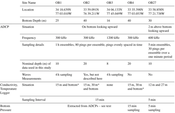
Table 1. Configuration of CORMP Instrumentation.
Site Name OB1 OB2 OB3 OB4 OB27 Location 34 18.639N 33 59.091N 34 06.133N 33 35.398N 33 58.858N
77 03.010W 76 39.211W 77 45.049W 77 03.053W 77 21.738W Bottom Depth (m) 25 40 16 40 30
ADCP Situation On bottom looking upward 2 m above bottom looking upward
Frequency 300 kHz 300 kHz 1200 kHz 300 kHz 600 kHz Sampling details 1 h ensembles, 80 pings per ensemble, pings evenly spaced in time 5 min ensembles,
30 pings per ensemble over a one minute period Nominal depth (m) of 10 20 8 20 10
data used in this study
Waves 4 h sampling Yes, but not 4 h sampling No No Measurements described here
Conductivity, Situation 15 m and bottom* 15 m, 30 m* none 15 m, 30 m 12 m and 27 m Temperature and bottom and bottom*
Logger
Sampling Interval 15 min 5 min Bottom Extracted from ADCPs – see text 15 min 5 min
Pressure sampling sampling
* Conductivity/salinity data not discussed or shown for these instruments due to data quality problems.
storm near Cape Hatteras. In Onslow Bay, the maximum wind speeds close to landfall were 30–35 m/s offshore of Beaufort, NC. Winds speeds over most of our observational array were 20–30 m/s at their height near the time of land-fall. Winds were nearly uniform in direction and speed over Onslow Bay, making the direct measurements at FPT a good proxy for winds over the entire Bay.
Onslow Bay is part of the Carolina Capes region (Pietrafesa et al., 1985a) between Cape Fear and Cape Look-out on the coast of North Carolina (Fig. 1). Flows in Onslow Bay are dominated at high frequencies by semidiurnal tides, which are predominantly across-shelf and make up to 80% of the kinetic energy at mid-shelf (Pietrafesa et al., 1985b). At lower frequencies, in normal times, flows are mainly as-sociated with Gulf Stream meanders on the mid- and outer shelf and wind events on the mid- to inner shelf.
As part of the Coastal Ocean Research and Monitoring Program (CORMP), the University of North Carolina at Wilmington and North Carolina State University maintained an array of moorings at 5 sites in Onslow Bay (Fig. 1 and Table 1) which collected data during the storm. Each in-strumented site had an RD Instruments Workhorse acoustic
Doppler current profiler (ADCP) placed on or near the bot-tom looking upwards. Instrument details including sampling intervals can be found in Table 1.
Current records were extracted from the ADCP data at the depths shown in Table 1. Currents at OB1-4 were spline-interpolated to 15 min before low-pass filtering. Currents at OB27 were subsampled at 15 min intervals before low pass filtering. In general, for periods greater than 2 h, the flows in the time around the storm were largely barotropic, as will be shown later, so the results presented here are not sensitive to choice of depth. Currents were low-pass filtered using a Butterworth filter with a cutoff of 24 h. High-pass currents at OB27 were calculated with a Butterworth filter with a cutoff of 5 h using the 5 min data.
Directional wave data were collected by the ADCP instru-ments at OB1 and OB3 (Table 1). (Directional wave data were also collected at OB2 but are not discussed here due to data quality problems.) Directional waves were measured ev-ery 4 h, using 18 min bursts at 2 pings/s. Processing was done using RD Instruments’ WavesMon software. Directional spectra are calculated with the velocity profile method (RD Instruments, 2005) and displayed using software developed
23 Figure 2
Fig. 2. Wind speed and direction at FPT. Dotted line shows time of
landfall.
at the University of South Carolina (G. Voulgaris, personal communication). Swell was separated from wind waves us-ing a cutoff of 8 s period.
Pressure data were extracted from waves-upgraded AD-CPs at OB1-3. Pressure data were recorded by the instru-ments at 2 Hertz over 20 min bursts once every 4 h. The pres-sures were averaged into ensembles with nominal recorded times at 10 min past the hour every 4 h. They were spline-interpolated to 15 min intervals, and low-pass filtered with the same filter as was used for the velocity data.
Temperature, conductivity/salinity and bottom pressure were also recorded at a number of locations (Table 1). In-struments used were either Seabird SBE37 Microcats or SBE19 Seacats. Bottom pressure measurements from OB4 and OB27 were low-pass filtered using the same filter as for the velocity data.
AVHRR sea surface temperature images were obtained from Rutgers University’s online archive (http://www. thecoolroom.org).
3 Results
All variables were examined in a 7 day period surrounding the approach and departure of Isabel, 15–22 September 2003. After about the beginning of the day on 20 September all quantities appeared to have returned to their normal level of variability.
3.1 Winds (Animations 1 and 2 and Figs. 2 and 3)
Winds at Frying Pan Tower were light and steady out of the north and northeast before the arrival of Isabel (Animation 2). They began to increase in speed around the middle of 16
24
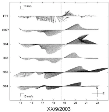
Fig. 3. Stick diagram of winds at FPT (top series) and low-pass
currents at other moorings as shown at left. A scale for the winds is shown at the top left and for the currents at bottom left.
September. Between 12:00 on 16 September and 12:00 on 17 September, the wind increased steadily but the direction did not change much. Around 12:00 on 17 September, the wind direction began to back slowly towards the north. At 00:00 on 18 September, the wind direction began to back rapidly as the storm approached, from north around to northwest and west. At landfall the wind was from the west southwest and rotating rapidly. After landfall, the wind rotated until it was from the south at 03:00 on 19 September, and then dimin-ished quickly. By 00:00 on 20 September, the winds became light and variable, showing no further signs of the storm.
Figures 2 and 3 have the same data in a different per-spective, showing the magnitude and direction and the wind sticks. Here we can see the gradual rise and quick decrease of the wind speed along with the rapid rotation during be-tween 00:00 on 18 September and 03:00 on 19 September. Maximum sustained winds at FPT were 32 m/s at 18:00 on 18 September.
Animation 1 shows the wind field every three hours near the time of landfall. It indicates that the winds were rela-tively uniform across Onslow Bay when they were at their highest though the winds closer to the eye of the storm ro-tated somewhat faster than winds further away as the storm made landfall.
3.2 Temperature (Figs. 4 and 6)
Waters in OB were warm during Isabel, ranging from 24 to 28◦C. Stratification was very small and temperature
25 Fig. 4. Temperature at 4 moorings during the period surrounding the
landfall of Hurricane Isabel. Green curves are bottom instruments (27 m at OB27). Blue curves are 15 m instruments (12 m at OB27) and red curves are 30 m instruments (see Table 1). Note different temperature scales for different moorings. Dotted line shows time of landfall.
differences were minimal for the entire period. (This is not typical for this time of year. Shelf waters are often highly stratified in late summer and early fall.) The exception to that is offshore at OB2 and especially OB4 which show some stratification near the surface. Most typical is the record at OB27. Before Isabel, the temperature was relatively constant at around 26–26.5◦C. As Isabel approached, the temperature
dropped about 2◦C to a minimum of 24◦C just after
land-fall. It then rose again to a constant level of 25.5◦C. Thus,
in the period before and after Isabel, the water column de-creased in temperature by 0.5◦C. OB1 shows some similar
but inverse behavior. During the storm, the temperature actu-ally increased, but then dropped again to a level about 0.1◦C
cooler than before the storm. At OB2 and OB4, the picture is more complicated. OB4 showed no particular storm effects on temperature. If the beginning of 20 September is chosen as the “after-storm” time, the temperature appears to have in-creased slightly during the storm. For OB2, the temperature decreased by 2◦C, again if 20 September is the after-storm
time. Satellite temperatures largely confirm the lack of strat-ification except at OB1 before the storm where the surface was about 2◦C warmer than the mid-depth and bottom
moor-ings.
78° W 77° W 76° W
33° N 34° N 35° N
Fig. 5. Progressive vector diagrams starting on 15 September 2003
for low pass current at mooring locations detailed in Fig. 1 and Ta-ble 1. The passage of time is indicated by coloration. The line turns from red on 15 September 2003 gradually into blue on 22 Septem-ber 2003.
The temperatures shown in Fig. 4 do not represent a single water mass. Some of the temperature changes seen in Fig. 4 are possibly due to advection of warmer or cooler water. A progressive vector diagram (PVD) was created from the low pass currents for OB27 (Fig. 5). This analysis indicated that waters initially at OB27 were advected 30 km to the south-west during the first part of the storm and then advected back during the latter part. The final position from the PVD on 22 September is within 1 km of the initial position on 15 September. In other words, water advected away from OB27 during storm and advected back as it departed. Assuming that this is true, and also assuming the entire water column was completely mixed, we can use the change in tempera-ture and the water depth to get an estimate of the net heat flux. Hurricane Isabel’s winds impacted OB for about 24 h. If we use this time period and the water depths in Table 1, we get a net heat flux of 750 W/m2at OB27. Although there is no way to verify this number, or provide error bounds, it is certainly a plausible estimate of the heat flux during a storm event like this (Jacob et al., 2000).
To get a larger picture of the temperature field on the shelf, we examined before and after AVHRR SST images (Fig. 6a– c). The before image shows a nearshore plume of cool water moving down the coast around Cape Hatteras just past Cape Lookout. This is a typical feature for this area (Pietrafesa et al., 1994). A cold core Gulf Stream filament is impinging on
27
28 Figure 6b
29
Fig. 6. (a) AVHRR MCSST Temperature (◦C) image from 15
September 2003 at 22:00. Colorbar at right indicates temperature scale. Locations of CORMP moorings and FPT are shown on map (see Fig. 1). (b) Same as (a) but for 19 September 2003 at 22:54.
(c) Temperature difference between (a) and (b).
30
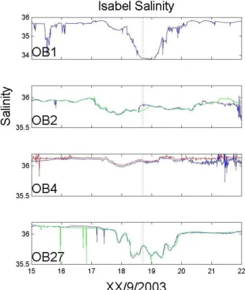
Fig. 7. As in Fig. 4, but for salinity. Note some records are not
plotted because data were not of acceptable quality to present (see Table 1). Dotted line shows time of landfall.
the continental shelf. Its warm streamer is especially vis-ible at OB2 and OB4. Again this is typical for this area (Pietrafesa et al., 1985a). The after-storm image (Fig. 6b), shows significant cooling of the inner shelf. The warm wa-ters associated with the Gulf Stream in the before-storm im-age are further from shore. The Gulf Stream filament is not apparent. The image showing the after-before temperature difference (Fig. 6c) indicates that the magnitude of the cool-ing across the shelf is approximately 1–3◦C. The cooling is
mainly confined inshore of OB2 and OB4. Even greater cool-ing occurred northeast of Cape Lookout under the track of the storm and offshore of the nearshore plume mentioned above. 3.3 Salinity (Fig. 7)
Salinity records indicate that salinity was relatively constant and uniform across the mid- and outer shelf prior to the approach of Isabel. Like temperature, there was no salin-ity stratification during the period of the storm. Late on 17 September, salinity began to drop at all 4 moorings with con-ductivity sensors. At OB2 and OB4, on the outer shelf, the drop was slight, perhaps 0.1 at the most. At OB27 salinity dropped about 0.5, to a minimum of about 35.6 late on 18 September. At OB1, salinity reached a minimum of 33.8 late on 18 September, having dropped almost 2.0 from its pre-storm level. The salinity at OB1 and OB27 then rebounded
31
Fig. 8. Unfiltered bottom pressure at OB4 and OB27. Dotted line
shows time of landfall.
during 19 September and reached a nearly constant level early on 20 September.
In order to understand these salinity records, we did the following calculation for the record at OB27. We assume, as we did for temperature, that the salinities early on 17 Septem-ber and early on 20 SeptemSeptem-ber represent the same water. That is, water present on 17 September advected away from the site during the storm and then returned approximately by 20 September. During this time, there was storm-related pre-cipitation, which fully mixed in. There was a difference in salinity of about 0.1 between 17 September and 20 Septem-ber. This change in salinity spread out over a 30 m depth represents a net addition of about 8 cm of water at the sur-face. In other words, given a 30 m high column of water of unit surface area, the addition of 8 cm of fresh water at the surface, when fully mixed in, would cause a change in salin-ity of −0.1.
Note that the salinity change between 17 September and the minimum late on 18 September is about 0.5. If this were the same water this would represent a net precipitation of about 41 cm. This is far too high a value to be plausible given the rainfall measured nearby on land (Beven and Cobb, 2004). Thus, we have to guess that the large drop in salinity was not entirely a result of net precipitation, but must be due at least in part to advection.
Using the previously quoted heat flux value of 750 W/m2 at OB27 over a period of 24 h (and assuming this is en-tirely due to latent cooling) gives an evaporation from the surface of about 3 cm. Thus, with a net addition of 8 cm of water to the surface, and 3 cm of evaporation, we calculate 11 cm of rainfall. The National Weather Service Forecast Office in Wilmington, NC reported a total rainfall of 5.03 cm (1.98′′) while Beven and Cobb (2004) reported 4–7 inches
(10–18 cm) throughout eastern North Carolina. For 11 cm of rain spread out over 24 h, the rain rate would be calculated as almost 5 mm/h.
32
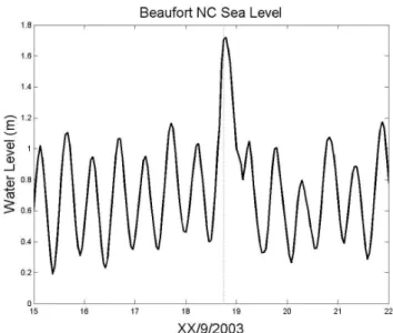
Fig. 9. Sea level at Beaufort Inlet, NC. Dotted line shows time of
landfall.
3.4 Pressure and sea level (Figs. 8, 9 and 10)
Bottom pressures at OB4 and OB27 showed no indication of storm surge on the mid- and outer shelf (Fig. 8). The records are somewhat aliased, having been sampled at 15 and 5 min intervals (Table 1) underneath an energetic field of surface waves. The surface wave field was apparent as a large in-crease in high frequency variability as the storm approached. The pressure sensors at OB4 and OB27 were at about 40 and 28 m depth. At this depth, pressure sensors only de-tect signals from surface waves of periods 8–10 s or greater, i.e. swell. Thus, the high frequency variability is a measure of the energy in the swell. Interestingly, this high frequency variability died down at OB4 around the end of the day on 17 September, almost a day earlier than it did at OB27. As we will see later, the high frequency variability of the pres-sure at OB27 decreased at about the same time as the swell energy at OB1. The high frequency variability at OB4 also increased much sooner than OB27. It is not clear whether the difference between the pressure records at the two locations is a result of the geographic difference between them, the dif-ferent depths of the sensors, or local topographic variations that might have focused or diffused the swell arriving from the distant storm.
By contrast, sea level at Beaufort Inlet, NC (Fig. 9) showed a storm surge of about 70 cm above predicted high tide. The highest sea level at Beaufort was reached at 19:00 on 18 September. Sea level was also measured at other locations along the coast. For example, at Cape Hatteras Fishing Pier, near the eye of the storm shown in Fig. 1, storm surge reached 2 m above the predicted tide at 14:00 on 18 September, when the tide gauge ceased to operate. Storm surge caused the opening of a new inlet in the Outer Banks near Cape Hat-teras Village, NC (Keen et al., 2005).
33 Figure 10
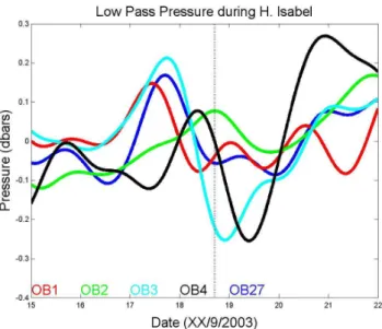
Fig. 10. Low pass bottom pressure. Each record has had the 15–
22 September mean subtracted from it. Different colored lines are from different moorings, with the color codes at the bottom of the figure. Dotted line shows time of landfall.
Low pass bottom pressures (Fig. 10) show no sign of mid-shelf storm surge. The records at OB3 and OB27 are similar as they are near each other. The outer shelf records (OB2 and OB4) are different from the inner shelf records.
3.5 Low Pass Current (Animation 2 and Figs. 3, 11 and 12) Before the arrival of Isabel, the low pass currents at all moor-ings were weak and slowly rotating counterclockwise. They maintained this motion until 06:00 on 16 September. At that time, current vectors at all of the moorings suddenly turned and pointed towards the southwest. By 00:00 on 18 Septem-ber, currents at all moorings were pointed towards the south-west and increasing in speed. There is an indication through-out that currents were turning along the shelf to follow the cuspate shape of the coastline. For example, the current at OB1 pointed more towards the west than that at OB3. The currents all reached their maximum speed towards the south-west around 09:00 on 18 September. At that point, the cur-rents began to diminish rapidly. The current speeds at all the moorings reached their minimum at nearly the same time, around 19:00–22:00 on 18 September (Table 2). The cur-rents then increased rapidly in speed towards the northeast, reaching maximum speed about 12:00 on 19 September. Af-ter this point, currents at the inner and mid-shelf moorings diminished rapidly. At the offshore moorings current speeds remained high, but the two moorings seemed to lose their coherence. After the passage of the storm, currents began to behave independently at the different moorings, in sharp contrast to the high coherence displayed between 06:00 16 September and 12:00 19 September.
34
Fig. 11. Low pass current speed and direction at OB27. Dotted line
shows time of landfall.
Figure 11 displays the same information in a different way for OB27 only. Here one can see the increase in speed to-wards the southwest after 06:00 16 September to a maximum of 32 cm/s at 05:45 on 18 September. There is a rapid rever-sal towards the northeast with the speed going to a minimum at 20:30 on 18 September. The maximum towards the north-east is reached at 11:15 19 September.
The vertical distribution of low pass flow at OB27 (Ani-mation 3) highlights the relative depth invariance of the low pass flows. In particular as the flow accelerated towards the southwest before the storm’s arrival, the entire water column moved in essentially the same direction. After the reversal, the flow moved again in the same direction towards the north-east, but as the flow slowed down the deeper flows rotated clockwise relative to the shallow flows. This would be an in-dication of the importance of bottom friction in slowing the flow down after the event was over.
With water across the shelf moving as a slab, the low pass flows seemed to be confined to the alongshore direction. In the hours before the flow reversal (17:00 17 September– 09:00 18 September), the currents appeared to rotate a lit-tle bit in the same direction as the wind, but are mainly along-shelf. The flow reversal occurs just as the wind ro-tated enough to where its along-shelf component is upshelf rather than downshelf. That is, the reversal occurred just as the wind vector rotated through a direction more or less per-pendicular to the coast. This suggests that the currents were mechanically forced by the wind as it picked up on 16 and 17 September. Ekman dynamics then became important as the steady north wind had blown long enough for the Corio-lis force to have an effect. When the wind began to rotate rapidly with the approach of the storm, direct mechanical forcing again dominated, this time pushing the shelf waters towards the northeast.
35 Figure 12
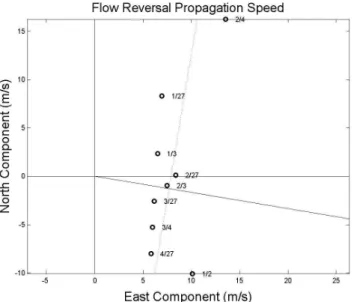
Fig. 12. Propagation of the flow reversal across the CORMP array.
Individual points are labeled with the appropriate pair of moorings. For example, point labeled “1/27” shows the speed and direction of propagation of the flow reversal from OB1 to OB27. Dotted line is a least squares fit to the points shown. Solid line points 10◦below
the x-axis, perpendicular to the dotted line.
Progressive vector diagrams for all of the moorings (Fig. 5) confirm this view. For each mooring, the flow sped off towards the southwest as Isabel approached, and changed direction back towards the northeast as it departed. The max-imum total displacement implied is about 30 km southwest. At all moorings, progressive vector diagrams indicate flow having returned to very close to the mooring location by the end of the study period, except for OB2, which overshot its original location.
The flow reversal occurred abruptly but not uniformly across the shelf. We used the time at which the speed goes to a minimum (Table 2) as the approximate time of the rever-sal at each mooring. Generally the reverrever-sal proceeded up the coast from southwest to northeast and inshore to offshore. OB3 was first, OB27 second, then OB1 and the two offshore moorings. The greatest difference between times was 03:45 between OB3 and OB2. Each of these time differences im-plies a propagation speed and direction. This information is presented in Fig. 12. We can think of the CORMP moorings as an array through which a signal has propagated and been received at each mooring at the time of the flow reversal. The speed of propagation is the projection of the velocity vectors shown in Fig. 12 onto the real direction of propagation. If the signal were a pure unidirectional plane wave going with con-stant direction and speed, each velocity derived from a moor-ing pair would have the same projection. Thus all would lie on the a line and the direction of propagation would be per-pendicular to that line.
Table 2. Time on 18 September when the flow speed becomes a
minimum at each mooring.
OB1 OB2 OB3 OB4 OB27 21:45 22:45 19:00 22:00 20:30
For reference, two lines are added to the figure. One is a least squares fit to the data in the plot. The other goes from the origin 10◦to the south of east and is perpendicular to the
dotted line. If the flow reversal were a perfect plane wave all the points in Fig. 12 would lie exactly on the dotted line, and the point of intersection of the two solid and dotted lines would have coordinates of the velocity vector with which the wave propagates. The propagation associated with OB3, the shallowest mooring, was apparently slower than this line would indicate, while the propagation associated with OB2 and OB4, the deeper moorings were faster. This suggests that the propagation sped up as it moved from the inner to the outer shelf, as expected for a shallow water wave.
Obviously, the flow reversal was not a pure plane wave. The direction and speed could have changed due to refrac-tion from changing bottom depth. The propagarefrac-tion speed is somewhat slower than the local shallow water wave speed, c=√(gH), where g is gravity and H is the depth. If the bottom depth is 15–40 m, this gives wave speeds of 12–20 m/s. The direction of propagation is slightly to the south of east. This is close to directly offshore, about 33◦south of east. Thus the
flow reversal propagated in the offshore direction at nearly the speed of a shallow water wave Keen and Glenn (1999) have mentioned shown a hurricane disturbance creating a barotropic Kelvin wave. Here this is unlikely. A Kelvin wave would propagate along the coast, not across the shelf towards deep water. On the other hand, if the flow reversal were a pure shallow water wave, one would expect the water mo-tion associated with it to be in the direcmo-tion of propagamo-tion, not almost perpendicular. Finally, if the flow reversal were a Kelvin wave, one would expect a correlated response in the bottom pressure. Examination of bottom pressure at the moorings (Fig. 10) did not indicate any connection between the observed flow reversal and bottom pressure or bottom pressure gradient. If the response were a wave, one would expect the strong downshelf and subsequent upshelf flow to be accompanied by a reversal in pressure gradient. No indi-cation of a major change in along shelf pressure gradient can be seen in the low pass pressures. For example, one would expect the difference between OB2 and OB4 to change sign around the time of the storm landfall. However, that is not what is seen in Fig. 10. The same applies to the OB3-OB1 pressure difference. The flow reversal does not appear to be accompanied by a large-scale change in pressure gradient, which implies that the flows are not pressure-driven, but me-chanically pushed by the wind. The high pressures at OB3
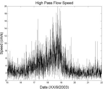
36 Fig. 13. Speed of the high pass flow at OB27.
and OB27 just before landfall might be an indication of water piling up in the southern part of Onslow Bay near Frying Pan Shoals by the push of the winds. This maximum in bottom pressure propagates to OB4 just about at the time of land-fall followed by a low in pressure at OB3 and OB4 as water sloshes out of the southern part of the Bay and towards the northeast.
A similar response was observed by Kohut et al. (2006) after Hurricane Floyd. The entire southern New Jersey con-tinental shelf flowed to the southwest along the coast before the arrival of the storm and it flipped around to the north-east after the storm’s departure. They describe this response as inertial, but not typical of the baroclinic clockwise rota-tion seen in deep water situarota-tions. The flow is seen in their model, driven by pressure gradients and quickly damped by bottom friction.
Another similar response is that documented by Keen and Allen (2000). They showed a disturbance created by Hurri-cane Andrew which propagated offshore in a path defined by the Mississippi Canyon. They described the disturbance as a Poincare (or Sverdrup) wave, essentially a low frequency shallow water wave influenced by rotation. However, some aspects of this event were different from what is described here. The disturbance is mainly defined by variations in inter-face height, something not observed in the pressure records in Onslow Bay. The disturbance traveled far more slowly than the one described in this paper and was confined to the canyon instead of being widespread across the shelf.
With all of the interesting detail in the low pass currents, we make note of the one thing that is missing. There was no apparent response in the inertial or near-inertial band, likely due to the lack of stratification.
37
Fig. 14. Significant wave height (m) at OB1 (solid) and OB3 (dashed). Dotted line shows time of landfall.
3.6 High pass current (Fig. 13)
The high pass currents at OB27 (from depth given in Ta-ble 1) intensified as the storm approached, reaching a max-imum amplitude of 10–12 cm/s close to the time of landfall and abruptly dying down afterwards. The increase in ampli-tude of the high frequency variability closely followed the increase in wind speed, the high frequency variability of the bottom pressure and the significant wave height (compare with Figs. 2, 8 and 14). Further analysis of the high-pass flow (not shown) showed that it was isotropic, and had ver-tical decorrelation scales of about 5 m. This high-pass flow was not simply aliased surface waves, because the sampling was specifically designed to remove the effects of surface waves by averaging over a one minute period (Table 1). The flows could conceivably be a result of the way that ADCP data were collected and calculated, with four acoustic beams averaged into each ensemble (Gordon, 1996). However, a similar type of flow has been observed in response to an im-pulsive wind in current data collected from a non-acoustic current meter (Klinck et al., 1981). Comparison of kinetic energy spectra from the time of the storm’s approach with spectra from a similar length calm period (not shown) indi-cate a significant elevation of kinetic energy at periods be-tween 10 min and 2 h. The OB27 instrument was not set up to measure flows with periods between 1 and 10 min, so some energy at these periods may not be apparent in this record.
We searched for vertical propagation of signals within this flow by doing time lag correlations between different bins of ADCP data. For example, we could not find significant correlations at any time lag between high frequency flows at 10 m and flow at 20 m. This suggests that these flows were not propagating signals up or down the water column. The
lack of stratification makes it unlikely that these flows were the result of internal waves.
3.7 Surface waves (Fig. 14 and Animation 4)
The significant wave height is calculated as four times the square root of the value obtained by integrating the non-directional spectrum from the time series of the surface level (RD Instruments, 2004). Thus, the square of the significant wave height gives an estimate of the total energy in the wave field as a function of time. Significant wave height at OB1 and OB3 show peak heights of close to 4 m at OB1 and 2– 2.5 m at OB3. The peak wave heights were reached at OB3 at 17 September at 16:00, and wave heights stayed high for over 24 h. Peak significant wave height at FPT (not shown) was reached at the same time as OB3 and was about 6 m. At OB1, the peak was reached just before Isabel made landfall on 18 September at 16:00. Note the wave field was sam-pled only every 4 h, making determination of the peak wave height and timing inexact. At OB1, the wave heights built up slowly over 3–4 days, until landfall, and then dropped abruptly during the day on 19 September. At OB3, the in-crease and dein-crease were more symmetric.
Animation 2 presents directional wave data as a func-tion of time for OB1. (An animafunc-tion from OB3 is omitted for brevity because the results were similar.) Even on 15 September, the energy in the swell was elevated as the storm produced waves far away in the North Atlantic. The swell built up as the storm approached and reached a maximum level around 12:00 on 17 September (bottom left panel). Af-ter that, the swell energy decreased. For most of the time there was a clear spectral gap between the swell and wind waves (top left panel).
The wind wave spectrum started out small and did not start building up until about 16:00 on 16 September. At that time the wind waves were coming from the east, while the wind itself was out of the north-northeast. The wind waves con-tinued to build, coming mainly from the east, until 04:00 on 18 September. After that, the wind direction began to rotate rapidly. The principal direction of the wind waves followed the rotation of the wind direction, staying 45–90 degrees behind the wind as it rotated. From the directional spec-trum on 18 September, it appears the high frequency wind waves rotated in direction more quickly than the lower fre-quency wind waves. Note especially the directional spectrum at 08:00 on 18 September. The wind waves reached a peak at 00:00 on 19 September when the wind wave direction was the same as that of the wind, out of the southwest. At that point, the wind wave field diminished quickly to very low levels. There was very little wave energy in the wind waves or the swell by 00:00 on 20 September. The build-up of wind wave energy followed closely the increase of wind speed at FPT.
It is of note here that the wind wave energy and the swell energy peaked 36 h apart, the wind waves at 00:00 on 19
September and the swell at 12:00 on 17 September. The to-tal energy in the wave field peaked somewhere in the middle, near the time of landfall as indicated by the significant wave height. The composition of the wave field changed dramat-ically in frequency and direction throughout the duration of the event.
4 Discussion
Hurricane Isabel was a significant low frequency current event in Onslow Bay, but hardly exceeded the normal pres-sure and current fluctuations of the tides. The storm moved quickly, but due to its huge size impacted Onslow Bay for a long period of time. Wind speeds were over 10 m/s for about 3 days (Fig. 2). Speckhart (2004) examined the ef-fects of three hurricanes, Dennis, Floyd and Irene, on On-slow Bay in 1999. Of the three, Dennis had the strongest effect on temperature and dynamics. This was not because it had the strongest winds, but because of the long duration of high winds. Dennis sat nearly motionless for several days offshore of Cape Hatteras while nearly steady 10 m/s winds blew over the Bay. Examination of the four year record we have of flows at OB27 indicates that Hurricane Isabel was a particularly energetic event in terms of the larger-scale low frequency response presented in the Animation 2. We spec-ulate that this is a result of the size and duration of the event as opposed to the magnitude of the winds.
In the fall, the water column in Onslow Bay normally be-gins to cool gradually as part of the seasonal cycle. However, that cooling mainly occurs in November and December, well after the passage of Isabel. While the 0.5◦C drop in
tem-perature at OB27 (Fig. 4) is associated with the large latent heat flux due to the storm, the size of the change is small compared to fluctuations normally observed at the site. Tem-perature can change because of seasonal cooling or heating, the passage of fronts, both oceanic and atmospheric, and the upwelling of cool water from the shelf edge. Examination of temperature records leads to the conclusion that while Hur-ricane Isabel had a large temporary effect, in general such storms are a small part of the heat budget for Onslow Bay. The same conclusion can be made for salinity and the fresh-water budget.
In terms of the impact on sediments and biota, the most important effect of the storm was in the wave field. Mar-shall (2004) reported wave orbital velocities of 60–70 cm/s at OB27 at the height of Isabel. This is far higher than the 20–30 cm/s amplitude of the tides or the 30 cm/s amplitude of the low frequency response shown in Figs. 3, 11 and An-imation 2. As Marshall reported, this made Isabel an ex-tremely unusual event in its ability to mobilize find-grained sediments.
While some aspects of the ocean’s response to Isabel re-main unexplained, what is clear from this study is the value of a well-designed and instrumented array to understanding
the impact that such storms can have on the coastal ocean. As more such arrays are built under the auspices of the Inte-grated Ocean Observing System (IOOS), we will have many more opportunities to study how storms like Isabel change the ocean environment that they pass over.
Appendix A Animation 1
(http://www.ocean-sci.net/3/159/2007/
os-3-159-2007-supplement.zip). Wind vectors from the National Hurricane Center’s Hurricane Isabel model. Snapshots are every three hours. A 20 m/s scale is shown at the top and the time and date at bottom.
Animation 2
(http://www.ocean-sci.net/3/159/2007/
os-3-159-2007-supplement.zip). Hourly wind and low pass currents in Onslow Bay, NC. Black circles represent mooring locations OB1-4 and 27 (see Fig. 1). Low pass currents are displayed as blue vectors with tails at mooring locations. The green dot is Frying Pan Tower, with hourly wind displayed as a green vector. Scale bars are shown in upper left, blue for current and green for wind. Hurricane track is shown as blue circles. Double blue circles are positions of the eye of Hurricane Isabel obtained from the Hurricane Research Division. Single blue circles are interpolated positions at times between the given positions at the double blue circles. The time and date of each frame are shown at the lower left. Towards the end of the animation, the hurricane eye can be seen moving through the frame to the northwest as a series of red circles that progressively cover the blue track as the eye passes.
Animation 3
(http://www.ocean-sci.net/3/159/2007/
os-3-159-2007-supplement.zip). Vertical profiles of low pass current from OB27. Each stick represents the flow in a particular 1 m bin. The color changes from red to blue progressing upward in the water column. The reddest (bluest) stick shows the flow at about 25 (5) m depth. A 10 cm/s scale is shown at the top, and the time and date are shown at the bottom.
Animation 4
(http://www.ocean-sci.net/3/159/2007/
os-3-159-2007-supplement.zip). Directional wave spectral information from OB1. Time and date are indicated at the top left. Upper left panel. Wave spectra integrated over direction as a function of frequency. The boundary between the red and blue parts of the curve at f=1/8 s is taken to be the boundary between the wind waves (red) and the swell (blue), Lower left panel. Wave spectra integrated over frequency as a function of direction. Direction for waves is where they
come from. Blue is the swell and red is the wind waves as defined in the upper left panel. The black line is the wind (from) direction. The position of the black dot that moves up and down on this line is proportional to the wind speed. Right panel. Full directional spectrum, with color bar at bottom.
Acknowledgements. Mooring data were collected under the
auspices of CORMP, which is funded by NOAA. Technical support with data collection was provided by J. Souza, D. Wells, B. Sweet, J. Kinder, and others. The code for displaying the waves data was generously provided by G. Voulgaris. Model wind data in Fig. 1 and storm track data in Animation 1 were downloaded from NOAA’s Hurricane Research Division. AVHRR data in Fig. 6 were provided by Rutgers University’s Coastal Ocean Observation Lab, with special help from J. Bosch. I had helpful comments from M. Durako, G. Snedden and J. Morrison and two anonymous reviewers.
Edited by: E. J. M. Delhez
References
Beven, J. and Cobb, H.: Tropical Cyclone Report, Hurricane Is-abel, 6–19 September 2003, National Hurricane Center, Miami Fl, 2004.
Chu, P. C., Veneziano, J. M., Fan, C., Carron, M. J., and Liu, W. T.: Response of the South China Sea to Tropical Cyclone Ernie 1996, Jour. Geophys. Res. C Oceans, 105(C6), 13 991–14 009, 2000.
Geisler, J. E.: Linear Theory of the Response of a Two Layer Ocean to a Moving Hurricane, Geophys. Fluid Dyn., 1, 249–272, 1970. Ginis, I. and Sutyrin, G. G.: Hurricane-generated Depth-averaged Currents and Sea Surface Elevation, J. Phys. Oceanogr., 25, 1218–1242, 1995.
Gordon, R. L.: Acoustic Doppler Current Profiler Principles of Op-eration A Practical Primer, 1–54 pp., RD Instruments Inc., San Diego, 1996.
Jacob, S. D., Shay, L. K., Mariano, A. J., and Black, P. G.: The 3D Oceanic Mixed Layer Response to Hurricane Gilbert, J. Phys. Oceanogr., 30(6), 1407–1429, 2000.
Keen, T. R. and Glenn, S. M.: Shallow water currents during Hur-ricane Andrew, J. Geophys. Res. (C Oceans), 104(C10), 23 443– 23 458, 1999.
Keen, T. R. and Allen, S. E.: The Generation of Internal Waves on the Continental Shelf by Hurricane Andrew, J. Geophys. Res. (C Oceans), 105(C11), 26 203–26 224, 2000.
Keen, T. R., Rowley, C., and Dykes, J.: Oceanographic Factors and the Erosion of the Outer Banks during Hurricane Isabel, from Hurricane Isabel in Perspective, edited by: Sellner, K., Chesa-peake Bay Research Consortium, Edgewater, MD, 65–72, 2005. Klinck, J. M., Pietrafesa, L. J., and Janowitx, G. S.: Continental Shelf Circulation Induced by a Moving, Localized Wind Stress, J. Phys. Oceanogr., 11(6), 836–848, 1981.
Kohut, J. T., Glenn, S. M., and Paduan, J. D.: Inner Shelf Re-sponse to Tropical Storm Floyd, J. Geophys. Res., 111, C09S91, doi:10.1029/2003JC002173, 2006.
Marshall, J. A.: Event Driven Sediment Mobility on the Inner Con-tinental Shelf of Onslow Bay, NC, Masters Thesis, University of North Carolina Wilmington, 1–90, 2004.
Murray, S. P.: Bottom Currents Near the Coast during Hurricane Camille, J. Geophys. Res., 75(24), 4579–4582, 1970.
Pietrafesa, L., Janowitz, G. S., and Wittman, P. A.: Physical Oceanographic Processes in the Carolina Capes, in: Oceanogra-phy of the Southeastern U.S. Continental Shelf, edited by: Atkin-son, L. P., Menzel, D. W., and Bush, K. A., pp. 23–32, American Geophysical Union, Washington DC, 1985a.
Pietrafesa, L. J., Blanton, J. O., Wang, J. D., Kourafalou, V., Lee, T. N., and Bush, K. A.: The Tidal Regime in the South Atlantic Bight, in: Oceanography of the Southeastern U.S. Continental Shelf, edited by: Atkinson, L. P., Menzel, D. W., and Bush, K. A., pp. 63–76, American Geophysical Union, Washington DC, 1985b.
Pietrafesa, L. J., Morrison, J. M., McCann, M. P., Churchill, J., Boehm, E., and Houghton, R. W.: Water mass linkages between the Middle and South Atlantic Bights, Deep-Sea Res. II, 41, 365– 389, 1994.
Price, J. F.: Internal Wave Wake of a Moving Storm. Part I: Scales, Energy Budget and Observations, J. Phys. Oceanogr., 13, 949– 965, 1983.
Price, J. F.: Upper Ocean Response to a Hurricane, J. Phys. Oceanogr., 11, 153–175, 1981.
Price, J. F., Sanford, T. B., and Forristall, G. Z.: Forced Stage Re-sponse to a Moving Hurricane, J. Phys. Oceanogr., 24, 233–260, 1994.
RD Instruments Inc.: WAVES PRIMER: Wave Measurements and the RDI ADCP Waves Array Technique, 1–22 pp., RD Instru-ments Inc., San Diego CA, 2004.
Shay, L. K. and Chang, S. W.: Free Surface Effects on the Near-inertial Current Response to A Hurricane: A Revisit, J. Phys. Oceanogr., 27, 23–39, 1997.
Shay, L. K. and Elsberry, R. L.: Near-inertial ocean current response to Hurricane Frederic, J. Phys. Oceanogr., 17(8), 1249–1269, 1987.
Shay, L. K., Ellsberry, R. L., and Black, P. G.: Vertical Structure of the Ocean Current Response to a Hurricane, J. Phys. Oceanogr., 19, 649–669, 1989.
Smith, N. P.: Longshore Currents on the Fringe of Hurricane Anita, J. Geophys. Res., 83(C12), 6047–6051, 1978.
Smith, N. P.: Response of Florida Atlantic Shelf Waters to Hurri-cane David, J. Geophys. Res., 87(C3), 2007–2016, 1982. Speckhart, B. L.: Observational analysis of shallow water response
to passing hurricanes in Onslow Bay, NC in 1999, Masters The-sis, University of North Carolina Wilmington, 1–61, 2004. Walsh, E. J., Wright, C. W., Vandemark, D., Krabill, W. B., Garcia,
A. W., Houston, S. H., Murillo, S. T., Powell, M. D., Black, P. G., and Marks Jr., F. D.: Hurricane Directional Wave Spectrum Spatial Variation at Landfall, J. Phys. Oceanogr., 32(6), 1667– 1684, 2002.
Williams, W. J., Beardsley, R. C., Irish, J. D., Smith, P. C., and Limeburner, R.: The response of Georges Bank to the passage of Hurricane Edouard, Deep-Sea Res. (II Top. Stud. Oceanogr.), 48(1–3), 179–197, 2001.
Withee, G. W. and Johnson, A.: Data Report: Buoy Observations during Hurricane Eloise (September 19 to October 11, 1975), 21 pp., Washington, DC, 1988.
Wren, P. A. and Leonard, L. A.: Sediment transport on the mid-continental shelf in Onslow Bay, North Carolina during Hurri-cane Isabel, Estuar. Coast. Shelf Sci., 63(1–2), 43–56, 2005. Xie, L., Pietrafesa, L. J., Bohm, E., Zhang, C., and Li, X.: Evidence
and mechanism of Hurricane Fran-induced ocean cooling in the Charleston Trough, Geophys. Res. Lett., 25(6), 769–772, 1998.