Coupling the High Complexity
Land Surface Model ACASA to the
Mesoscale Model WRF
Liyi Xu , Rex Dave Pyles, Kyaw Tha Paw U,
Shu-Hua Chen and Erwan Monier
Report No. 265
August 2014
The MIT Joint Program on the Science and Policy of Global Change combines cutting-edge scientific research with independent policy analysis to provide a solid foundation for the public and private decisions needed to mitigate and adapt to unavoidable global environmental changes. Being data-driven, the Program uses extensive Earth system and economic data and models to produce quantitative analysis and predictions of the risks of climate change and the challenges of limiting human influence on the environment—essential knowledge for the international dialogue toward a global response to climate change.
To this end, the Program brings together an interdisciplinary group from two established MIT research centers: the Center for Global Change Science (CGCS) and the Center for Energy and Environmental Policy Research (CEEPR). These two centers—along with collaborators from the Marine Biology Laboratory (MBL) at Woods Hole and short- and long-term visitors—provide the united vision needed to solve global challenges.
At the heart of much of the Program’s work lies MIT’s Integrated Global System Model. Through this integrated model, the Program seeks to: discover new interactions among natural and human climate system components; objectively assess uncertainty in economic and climate projections; critically and quantitatively analyze environmental management and policy proposals; understand complex connections among the many forces that will shape our future; and improve methods to model, monitor and verify greenhouse gas emissions and climatic impacts. This reprint is one of a series intended to communicate research results and improve public understanding of global environment and energy challenges, thereby contributing to informed debate about climate change and the economic and social implications of policy alternatives.
Ronald G. Prinn and John M. Reilly,
Program Co-Directors
For more information, contact the Program office:
MIT Joint Program on the Science and Policy of Global Change Postal Address:
Massachusetts Institute of Technology 77 Massachusetts Avenue, E19-411 Cambridge, MA 02139 (USA) Location:
Building E19, Room 411 400 Main Street, Cambridge Access:
Tel: (617) 253-7492 Fax: (617) 253-9845
Email: [email protected]
Coupling the High Complexity Land Surface Model ACASA to the Mesoscale Model WRF Liyi Xu⇤†, Rex Dave Pyles‡, Kyaw Tha Paw U‡, Shu-Hua Chen‡and Erwan Monier⇤
Abstract
In this study, the Weather Research and Forecasting Model (WRF) is coupled with the Advanced Canopy-Atmosphere-Soil Algorithm (ACASA), a high complexity land surface model. Although WRF is a state-of-the-art regional atmospheric model with high spatial and temporal resolutions, the land surface schemes available in WRF are simple and lack the capability to simulate carbon dioxide (for example, the popular NOAH LSM). ACASA is a complex multilayer land surface model with interac-tive canopy physiology and full surface hydrological processes. It allows microenvironmental variables such as air and surface temperatures, wind speed, humidity, and carbon dioxide concentration to vary vertically.
Simulations of surface conditions such as air temperature, dew point temperature, and relative humidity from WRF-ACASA and WRF-NOAH are compared with surface observation from over 700 meteoro-logical stations in California. Results show that the increase in complexity in the WRF-ACASA model not only maintains model accuracy, it also properly accounts for the dominant biological and physical processes describing ecosystem-atmosphere interactions that are scientifically valuable. The different complexities of physical and physiological processes in the WRF-ACASA and WRF-NOAH models also highlight the impacts of various land surface and model components on atmospheric and surface con-ditions.
Contents
1. INTRODUCTION...1
2. MODELS, METHODOLOGY AND DATA...3
2.1 The Weather Research and Forecasting (WRF) Model...3
2.2 The Advanced Canopy-Atmosphere-Soil Algorithm (ACASA) Model...4
2.3 The WRF-ACASA Coupling...6
2.4 Model Setup...7
2.5 Data...8
3. RESULTS AND DISCUSSION...11
4. CONCLUSIONS...26
5. REFERENCES...28
1. INTRODUCTION
Although the earth is mostly covered by ocean, the presence of land surfaces introduces much complexity into the earth system that drives numerous atmospheric and oceanic dynamics. The effects of complexity ranges from the simple land-sea contrasts in radiation processes, to the wind flow dynamics, and to the more complex biogeophysical processes of terrestrial systems. Various types of plants, soils, and microbes, as well as all living organisms including humans are situated on and within the landscape that make up the earth’s terrestrial system of the bio-sphere. Though the surface layer represents a very small fraction of the planet—only the lowest
⇤Joint Program of the Science and Policy on Global Change, Massachusetts Institute of Technology, Cambridge,
MA.
†Corresponding author (Email:[email protected])
10% of the planetary boundary layer—it has been widely regarded as a crucial component of the climate system (Stull, 1988; Mintz, 1981; Rowntree, 1991). The interaction between the land sur-face (biosphere) and the atmosphere is therefore one of the most active and important aspects of the natural system.
Vegetation at the land surface introduces complex structures, properties, and interactions to the surface layer. Vegetation heavily modifies surface exchanges of energy, gas, moisture and mo-mentum, developing the microenvironment in ways that distinguishing vegetated surfaces from landscapes without vegetation. Such influences are known to occur on different spatial and tem-poral scales (Chen and Avissar, 1994; Pielke et al., 2002; Zhao et al., 2001). In particular, often near-geostrophically-balanced wind patterns are disrupted in the lower atmosphere when wind encounters vegetated surfaces, i.e., the winds slow down and change direction as a result of tur-bulent flows that develop within and near the vegetated canopies (Wieringa, 1986; Pyles et al., 2004).
Depending in part on the canopy height and structure, wind and turbulent flows vary consid-erably across different ecosystems—even when each is presented with the same meteorological and astronomical conditions aloft. Gradients in heating, air pressure, and other forcings develop across heterogeneous landscapes, helping to sustain atmospheric motion. Since the surface layer is the only physical boundary in an atmospheric model, there is a consensus that accurate simu-lations of atmosphere processes in an atmospheric model require detailed representations of the surface layer and its terrestrial system. Models that account for the effects of surface layer on cli-mate and atmosphere conditions are referred to as Land Surface Models (LSMs).
Unfortunately, the current land surface models, i.e., the widely used set of four schemes present in the Weather Research and Forecasting (WRF) model (5-layer thermal diffusion, Pleim-Xiu, Rapid Update Cycle, and the popular NOAH), often overly simplify the surface layer by using a single layer “big leaf” parameterization and other assumptions, usually based around some form of bulk Monin-Obukhov-type similarity theory (Chen and Dudhia, 2001a,b; Pleim and Xiu, 1995; Smirnova et al., 1997, 2000; Xiu and Pleim, 2001). These models scale the leaf-level physical and physiological properties as one extensive “big leaf” to represent the entire canopy.
The majority of the LSMs do not simulate carbon dioxide flux, even though it is largely recog-nized as a major contributor to the current climate change phenomenon and a controller of plant physiology. Plant transpiration in these models is often based on the Jarvis parameterization, in which the stomatal control of transpiration is a multiplicative function of meteorological vari-ables such as temperature, humidity, and radiation (Jarvis, 1976). However, a large number of studies show that there is a strong linkage between the physiological process of photosynthetic uptake and the respiratory release of CO2to plant transpiration through stomata (Zhan and Kus-tas, 2001; Houborg and Soegaard, 2004). As such, physiological processes related to CO2 ex-change rates should be included in surface-layer representation of water and energy exex-changes.
Oversimplification of surface processes and their impacts on the atmosphere in these land sur-face models will likely cause the models to misrepresent and poorly predict sursur-face–atmosphere interactions. Models in earth science fields that use simplified equations and statistical relation-ships to represent complex processes in physics, physiology, hydrology, and thermodynamics
require intense fine-tuning and optimization algorithms for their results to match observations (Duan et al., 1992). These empirical models are capable of producing results that are accurate to a certain extent, but their assumptions limit their ability to investigate relationships and feedback between different components of the system. For example, the empirical models are unable to characterize the relationship between canopy height and sub-canopy energy distribution, and the effects of increased carbon dioxide concentrations on vegetation-atmosphere interactions. This is especially true for regional scale studies, where the influence of the terrestrial system increases with better spatial resolution and heterogeneous land cover.
Recent computer and model developments have greatly improved atmospheric modeling abil-ities, as progressively more complex planetary boundary layer and surface schemes with higher spatial and temporal resolutions are being implemented. However, the challenges involved in ad-vancing the robustness of land surface models continue to limit the realistic simulation of plan-etary boundary layer forcings from vegetation, topography, and soil. Some have argued that the increase in model complexity does not translate into higher accuracy due to the increase in un-certainty introduced by the large number of input parameters needed by the more process-based models (Raupach and Finnigan, 1988; Jetten et al., 1999; de Wit, 1999; Perrin et al., 2001). How-ever, there is a certain scientific value in properly accounting for the dominant biological and physical processes describing ecosystem-atmosphere interactions—even if this greatly compli-cates the models.
This study introduces the novel coupling of the mesoscale WRF model with the complex mul-tilayer Advanced Canopy-Atmosphere-Soil Algorithm (ACASA) model, to improve the surface and atmospheric representation in a regional context. The objectives of this study are to (1) pa-rameterize complex land surface processes that drive local mesoscale circulations, and (2) to in-vestigate the effects of model complexity on accuracy.
2. MODELS, METHODOLOGY AND DATA
2.1 The Weather Research and Forecasting (WRF) Model
The mesoscale model used in this study is the Advanced Research WRF (ARW) model Ver-sion 3.1. WRF is a state-of-the-art, mesoscale numerical weather prediction and atmospheric research model developed by a collaborative effort of the National Center for Atmospheric Re-search (NCAR), the National Oceanic and Atmospheric Administration (NOAA), the Earth Sys-tem Research Laboratory (ESRL), and other agencies. The WRF model contains a nearly com-plete set of compressible and non-hydrostatic equations for atmospheric physics (Chen and Dud-hia, 2000) to simulate three-dimensional atmospheric variables, and its vertical grid spacing varies in height with smaller spacing between the lower atmospheric layers than the upper at-mospheric layers. The mass-based terrain following coordinate in WRF improves the surface pro-cesses. It is commonly used to study air quality, precipitation, severe windstorm events, weather forecasts, and other atmospheric conditions (Borge et al., 2008; Thompson et al., 2004; Powers, 2007; Miglietta and Rotunno, 2005; Trenberth and Shea, 2006). Compared to the 2.5◦
(equiva-lent to 250 km at the equator) resolution of General Circulation Models (GCMs), the WRF model with high spatial and temporal resolution is better suited for studying climate conditions over
California; WRF can be nested so that finer grid spacing (1 km or less) is possible.
As mentioned in the introduction, four different parameterizations of land-surface processes are available in the WRF model. WRF’s more widely used and most sophisticated NOAH em-ploys simplistic physics compared to ACASA, being more akin to the set of ecophysiological schemes that include SiB and BATS (Dickinson et al., 1993; Sellers et al., 1996). There is only one vegetated surface layer in the NOAH scheme, along with four soil layers to calculate soil temperature and moisture. The “big leaf” approach assumes the entire canopy has similar phys-ical and physiologphys-ical properties to a single big leaf. In addition, energy and mass transfers for the surface layer are calculated using simple surface physics (Noilhan and Planton, 1989; Holt-slag and Ek, 1996; Chen and Dudhia, 2000). For example, the surface skin temperature is lin-early extrapolated from a single surface energy balance equation, which represents the combined surface layer of ground and vegetation (Mahrt and Ek, 1984). Surface evaporation is computed using modified diurnally dependent Penman-Monteith equation from Mahrt and Ek (1984) and the Jarvis parameterization (Jarvis, 1976). The current WRF LSMs are relatively simple, when compared to the higher order closure based ACASA model, and none of them calculate carbon flux. In contrast, the fully coupled WRF-ACASA model is capable of calculating carbon dioxide fluxes as well as the reaction of the ecosystems to increases in carbon dioxide concentrations.
2.2 The Advanced Canopy-Atmosphere-Soil Algorithm (ACASA) Model
Compared to the simple NOAH, the ACASA model version 2.0 is a complex multilayer an-alytical land surface model, which simulates the microenvironment profiles and turbulent ex-change of energy, mass, CO2and momentum within and above ecosystems that constitute land surfaces. It represents the interaction between vegetation, soil and the atmosphere based on phys-ical and biologphys-ical processes described from the scale of leaves (microscale), and horizontal scales on the order of 100 times the ecosystem vegetation height (i.e., hundreds of meters to around 1 km). The surface layer is represented as a column model with multiple vertical layers extending to the lowest planetary boundary. The model has 10 vertical atmospheric layers above-canopy, 10 intra-canopy layers, and 4 soil layers.
For each canopy layer, leaves are oriented in 9 sun-lit angle leaf classes (random spherical ori-entation) and 1 shaded leaf class in order to more accurately represent radiation transfer and leaf temperatures in a simulated variable array. This array aggregates the exchanges of sensible heat, water vapor, momentum, and carbon dioxide. The values of fluxes at each layer depend on those from all other layers, so the longwave radiative and turbulence transfer equations are iterated until numerical equilibrium is reached. Shortwave radiation fluxes, along with associated arrays (prob-abilities of transmission, beam extinction coefficients, etc.) are not changed, while the other sets of equations are iterated to numerical convergence.
Plant physiological processes, such as evapotranspiration, photosynthesis and respiration, are calculated for each of the leaf classes and layers, based on the simulated radiation field and the micrometeorological variables calculated in the previous iteration step. The default maximum rate of Rubisco carboxylase activity, which controls plant physiological processes, is provided for each of the standardized vegetation types, although specific values of these parameters can be
entered. Temperature, mean wind speed, carbon dioxide concentration, and specific humidity are calculated explicitly for each layer, using the higher order closure equations (Meyers and Paw U, 1986, 1987; Su et al., 1996).
In addition to accounting for the carbon dioxide flux, a key advanced component of the ACASA model is its higher-order turbulent closure scheme. The parameterizations of the fourth-order
terms used to solve the prognostic third-order equations are described by assuming a quasi-Gaussian probability distribution as a function of second-moment terms (Meyers and Paw U, 1987). Com-pared to lower order closure models, the higher order closure scheme increases model accuracy by improving representations of the turbulent transport of energy, momentum, and water by both small and large eddies. In small-eddy theory or eddy viscosity, energy fluxes move down a local gradient; however, large eddies in the real atmosphere can transport flux against the local gradi-ent. Such counter-gradient flow is a physical property of large eddies associated with long dis-tance transport. For example, mid-afternoon intermittent ejection-sweep eddies cycling deep into a warm forest canopy with snow on the ground, from regions with air temperature values between that of the warm canopy and the cold snow surface, would result in overturning of eddies to trans-port relative warm air from above and within the canopy to the snow surface below. The local gradient from the canopy to the above-canopy air would incorrectly indicate sensible heat going upwards—instead of the actual heat flow down through the canopy—due to the long turbulence scales of transport. These potentially counter-gradient transports are responsible for much of land surface evaporation, heat, carbon dioxide and momentum fluxes (Denmead and Bradley, 1985; Gao et al., 1989). The ACASA model uses higher order closure transport between multiple lay-ers of the canopy to simulate non-local transport, allowing the simulation of counter-gradient and non-gradient exchange. By comparison, the simple lower order turbulent closure model NOAH has only one surface layer. It is limited to only down-gradient transport and cannot mix within the canopy.
In the ACASA model, both rain and snow forms of precipitation are intercepted by the canopy elements in each layer. Some of the precipitation is retained on the leaf surfaces to modify the microenvironment of the layers for the next time step, depending on the precipitation amount, canopy storage capacity, and vaporization or sublimation rate. The remaining precipitation is distributed to the ground surface, influencing soil moisture and/or surface runoff as calculated by the layered soil model. The soil model physics in ACASA are very similar to the diffusion physics used in NOAH, but ACASA includes enhanced layering of the snowpack for more de-tailed thermal profiles throughout deep snow. This multilayer snow model allows interactions be-tween layers, and more effectively calculates energy distribution and snow hydrological processes (e.g., snow melt) when surface snow experiences higher or lower temperatures than the under-lying snow layers. This is especially relevant over regions with high snow depth such as Sierra Nevada Mountain, where snow is a significant source of water. The multilayer snow hydrology scheme has been well tested during the SNOWMIP project (Etchevers et al., 2004; Rutter et al., 2009), where ACASA performed at least as well as many snow models by accurately estimating the snow accumulation rate as well as the timing of snow melt in a wide range of biomes.
across different countries, climate systems, and vegetation types. These include a 500-year old-growth coniferous forest at the Wind River Canopy Crane Research Facility in Washington State (Pyles et al., 2000, 2004), a spruce forest in in the Fichtelgebirge Mountains in Germany (Staudt et al., 2011), a maquis ecosystem in Sardinia near Alghero (Marras et al., 2008), and a grape vineyard in Tuscany near Montelcino, Italy (Marras et al., 2011).
2.3 The WRF-ACASA Coupling
In an effort to improve the parameterization of land surface processes and their feedbacks with the atmosphere, ACASA is coupled to the mesoscale model WRF as a new land surface scheme. The schematic diagram ofFigure 1 represents the coupling between the two models. From the Planetary Boundary Layer (PBL) and above, the WRF model provides meteorological variables as input forcing to the ACASA land surface model at the lowest WRF sigma-layer. These vari-ables include solar shortwave and terrestrial (atmospheric thermal long-wave) radiation, precip-itation, humidity, wind speed, carbon dioxide concentration, and barometric pressure. Radiation is partitioned into thermal IR, visible (PAR) and NIR by the ACASA model, which treats these radiation streams separately according to the preferential scattering of the different wavelengths as the radiation passes through the canopy. Part of the radiation is reflected back to the PBL ac-cording to the layered canopy radiative transfer model, with the remaining radiation driving the canopy energy balance components and photosynthesis.
Figure 1. The schematic diagram of the WRF-ACASA coupling.
Unlike the “big leaf” model NOAH, ACASA creates a normalized vertical Leaf Area Index (LAI) or Leaf Area Density (LAD) for the multiple canopy layers according to vegetation type.
This is crucial because the canopy height and distribution of LAD directly influence the interac-tions of wind, light, temperature, radiation, and carbon between the atmosphere and the surface layer.
2.4 Model Setup
The WRF model requires input data for prognostic variables including wind, temperature, moisture, radiation, and soil temperature, both for an initialized field of variables through the domain, and at the boundaries of the domain. In this study, these input data are provided by the Northern America Regional Reanalysis (NARR) dataset to drive both the NOAH and WRF-ACASA models. Unlike many other reanalysis data sets with coarse spatial resolution such as ERA40 (European Center for Medium-Range Weather Forecasts 40 Year Re-analysis) and GFS (Global Forecast System), NARR is a regional data set specifically developed for the Northern American region. The temporal and spatial resolutions of this data set are 3 hours and 32 km, re-spectively.
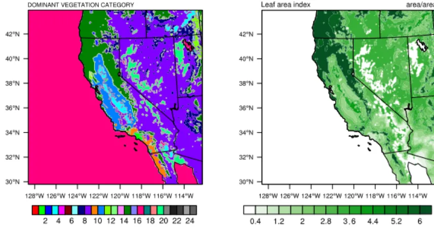
Simulations of both the default WRF-NOAH and the WRF-ACASA models were performed for two year-long simulations (2005 and 2006) with horizontal grid spacing of 8 km x 8 km. These years were chosen because they provide the most extensive set of surface observation data. The model domain covers all of California with parts of neighboring states and the Pacific Ocean to the west, shown inFigure 2. The complex terrain and vast ecological and climatic systems in the region make this domain ideal for testing the WRF-NOAH and WRF-ACASA coupled model performances. The geological and ecological regions extend eastward from the coastal range shrublands to the Central Valley grasslands and croplands, then to the foothill woodlands before finishing at the coniferous forests along the Sierra Nevada range. Areas further inland to the east and south include the Great Basin and Range Chaos, an arid and complex mosaic of forests and chaparral tessellated amid the myriad fossae that erupt between dunes and playas. The contrast-ing moist Northern and semiarid Southern California landscapes are also represented in tandem.
Figure 2. The complex topography and land cover of the study domain is represented here by: (left)
Dominant vegetation type and (right) Leaf Area Index (LAI) from USGS used by the WRF model. The horizontal grid spacing of 8 km is needed to resolve the major topographical and ecological features of the domain.
employ the same set of atmosphere physics schemes stemming from the WRF model. These in-clude the Purdue Lin et al. scheme for microphysics (Chen and Sun, 2002), the Rapid Radiative Transfer Model for long wave radiation (Mlawer et al., 1997), the Dudhia scheme for shortwave radiation (Dudhia, 1989), the Monin-Obukhov Similarity scheme for surface layer physics of non-vegetated surfaces and the ocean, and the MRF scheme for the planetary boundary layer (Hong and Pan, 1996). WRF runs its atmospheric processes at a 60-second time step, while the radiation scheme and the land surface schemes are called every 30 minutes. Because ACASA as-sumes quasi-steady-state turbulent processes, its physics are not considered advisable for shorter time intervals. Both NOAH and ACASA calculate surface processes and update the radiation bal-ance, as well as heat flux, water vapor flux, carbon flux, surface temperature, snow water equiv-alent, and other surface variables in WRF. Analytical nudging of four dimensional data assim-ilation (FDDA) is applied to the atmosphere for all model simulations in order to maintain the large-scale consistency and reduce drifting of model simulation from the driving field over time. Such nudging (FDDA) is commonly practiced in limited-area modeling, and current methods ac-tive in WRF are widely accepted due to rigorous testing (Stauffer and Seaman, 1990; Stauffer et al., 1991).
2.5 Data
The main independent observational datasets used to evaluate the model simulations were ob-tained from the Meteorological Section of the California Air Resource Board (ARB). The NARR data were not used for the evaluation as the dataset was used for FDDA during both model simu-lations. The ARB meteorology dataset is compiled from over 2000 surface observation stations in California from multiple agencies and programs: Remote Automated Weather Stations (RAWS) from the National Interagency Fire Center, the California Irrigation Management Information System (CIMIS), National Oceanic and Atmospheric Administration (NOAA), Aerometric In-formation Retrieval System (AIRS), and the Federal Aviation Administration. Potential measure-ment errors and uncertainties are expected in the ARB data because of the differences in station setups and measurement standards from the different agencies. For example, ambient surface air temperature is measured at various heights from 1 to 10 meters above the ground, depending on the measuring agency. Some stations are located in urban environments, while the model sim-ulations are structured to study natural vegetated environments. Therefore, some discrepancies between the observation and simulation are likely to occur in densely populated areas. How-ever, with hourly data from over 2000 observation stations within the study domain, the ARB dataset remains valuable. Out of the 2000 surface stations in the overall current ARB database, there were about 730 stations operational during the study period of 2005 and 2006 (Figure 3). The meteorological and surface conditions from the WRF-NOAH and WRF-ACASA model simulations were evaluated using the ARB data both for the regional scale level performance, and for specific stations for more in-depth analysis. This represents is the most rigorous test of ACASA to date, in terms of the sheer number of ACASA point-simulations and the number of ACASA points linked in both space and time. This investigation therefore represents a significant elaboration upon earlier work (Pyles et al., 2003). Meteorological variables such as surface air
Figure 3. Map of the location of the California Air Resources Board surface stations.
temperature, dew point temperature, and relative humidity from the two model simulations were compared with each other and the observational data. Four basins within the study domain were selected to represent the different vegetation covers and geographic locations within the domain: the Northeast Plateau (NEP) is mostly grassland that covers 32 percent of the landscape; the Mo-jave Desert (MJ) station located at the southeastern California is mostly shrubland with a 13.75 percent of vegetation cover; the San Joaquin Valley (SJV) is a major agricultural region, covered by irrigated cropland and pasture with about 23 percent of the land covered by vegetation; and the Sierra Nevada Mountain County (MC) with 60 percent of the land covered by high-altitude vegetation (mainly evergreen needle leaf forest). These four basins encompass a total of 240 sta-tions. Measurements from these basins were compared to the WRF-NOAH and WRF-ACASA simulation outputs for the nearest grid points. From each basin, one station was identified for fur-ther detail analysis (seeTable 1).
Table 1. Selected sites from the Air Resources Board meteorological stations network. Basin Station ID Latitude Longitude PFT
NEP 5751 41.959 –121.471 Grassland
MD 5780 33.557 –114.666 Shrubland
SJV 5783 35.604 –119.213 Irrigated Cropland and Pasture
MC 5714 38.754 –120.732 Evergreen Needleleaf Forest
Hourly, daily and monthly data were used for model evaluation in this study. Due to the nature of continuous instrument network operations, however, data gaps are inevitable in surface ob-servations. To avoid missing data biases, only the days with complete 24-hour data sets are used for statistical analyses. The reason for this selection of data is illustrated inFigure 4. The black line in Figure 4 represents hourly temperature observations for the Mojave Desert Station during June 2006. The red line represents the daily mean temperature only from days with complete 24 hour sets of temperature observation. The black line contains data with missing gaps, which
in-fluence the mean monthly temperature calculation. The monthly mean temperature is lowered if it is calculated using only days with the complete 24 hours rather than all data. This is due to a significant amount of missing data from the daytime that skews the monthly temperature toward the cooler nighttime temperature, resulting in a cold bias. By using only days with complete 24 hours of measurement for statistical analyses, the temperature bias toward any certain period of the day is avoided.
Figure 4. Time series of the surface air temperature at Mojave Desert Station during June 2006. The
black line represents the entire set of surface temperature observation with gaps presented. The red line represents the daily mean temperature calculated using only days with all 24 hours of observation available.
Some of the challenges in making a comparison between WRF-ACASA simulations and the observations are that (1) the observation heights were frequently different than the simulated grid point height, and (2) the station landscape type was often different than that of the simulation grid point. Many stations are within patches of specific landscape types that may differ significantly from the overall grid point landscape. Even more challenging is the fact that WRF-ACASA sim-ulations have outputs for the temperatures within a canopy, so for orchards or forests, the 2-meter height (surface) simulation data are not expected to match well with the 2-meter height observa-tions. For the taller plant ecosystems, WRF-ACASA simulations at the 2-meter height represent temperatures within the plant canopy or understory; yet, the observations from the ARB network are never in such locations. Rather, they are over other surfaces not representative of the simula-tion grid-point—and are usually not even at the 2-meter height. The WRF-NOAH simulasimula-tions do not suffer as much in terms of the 2-meter simulations; as the NOAH surface model is a big-leaf model, the 2-meter height includes characteristics more similar to that of the observations. De-spite these significant shortcomings, to maximize the number of observations, the ARB data were chosen because of the large number of stations throughout the simulation domain. The results from year 2005 and year 2006 are similar, so only year 2006 is presented here.
3. RESULTS AND DISCUSSION
The monthly mean surface temperatures in California from both model simulations are com-pared against the surface observations inFigure 5. The left panel shows the ARB data (gathered at approximately 10 m above the ground); the white areas represent regions with missing obser-vations. The WRF-NOAH and WRF-ACASA simulation outputs are represented in the center and right panels, respectively. The region’s geographical complexity is highlighted by the spatial and temporal variations in the surface temperature. The warm summer and cool winter are typ-ical of a Mediterranean-type climate. In addition to the seasonal variation, both WRF-ACASA and WRF-NOAH models are able to capture the distinct characteristics of the warm Central Val-ley and semiarid region of Southern California. The large, flat Central ValVal-ley is dominated by Irrigated Cropland and Pasture, and surrounded by Cropland/Grassland Mosaic. The cold tem-peratures over the mountain regions are also visible from the surface temperature field. However, there are noticeable differences between the WRF-ACASA and the WRF-NOAH over the Central Valley.
During the month of February, the WRF-ACASA output distinctly features a colder Central Valley surrounded by a slightly warmer region. A similar effect is also visible in the month of November, when WRF-ACASA again depicts a cold bias over the Central Valley. The tempera-ture contrast of this region is mostly due to differences in land cover type, as well as LAI associ-ated with the land cover (Figure 2). These two variables impact plant physiological processes in the WRF-ACASA model such as photosynthesis, respiration, and evapotranspiration. Lower LAI in the area immediately surrounding Central Valley results in less transpiration than in higher LAI Central Valley areas, which has higher partitioning of available energy to latent heat, and less to sensible heat.
MEAN SURFACE AIR TEMPERATURE (K)
Figure 5. Monthly mean surface air temperature simulated by WRF-ACASA and WRF-NOAH and for the
While the WRF-ACASA model is highly influenced by vegetation cover and the changes in LAI, the surface processes in WRF-NOAH rely heavily on the prescribed minimum canopy resis-tance for each vegetation type. Therefore, the contrast in temperature between regions of differ-ent vegetation cover and leaf area index is more pronounced in the WRF-ACASA model than the WRF-NOAH model. The overall agreement between the model simulations from WRF-ACASA and NOAH match well with surface observations throughout the year. However, the WRF-ACASA experiences a cold bias over the high LAI region in the Central Valley during the month of August. Once again, it should be noted that the WRF-ACASA output is generally not at the same height as the observation height, and the actual local vegetation type often differs from that immediately surrounding the observation sites. Close examination in the Central Valley also re-veals that the prescribed LAI values in WRF are significantly higher than the remote sensing LAI values during the summer months. Because WRF-ACASA relies on LAI to simulate plant physi-ological processes and energy budget, this discrepancy in LAI causes WRF-ACASA to overesti-mate evapotranspiration over the region and to create a cold bias. The WRF-NOAH model is less sensitive in this regard because it uses prescribed canopy resistances. This highlights the conun-drum of advancing model physics–more sophisticated models become more susceptible to errors in input data quality as they become more representative of variations in land cover type.
Figure 6 shows a time series of surface air temperature simulated by ACASA and WRF-NOAH alongside observations from four different stations in 2006 for the months of February, May, August, and November. Both WRF-ACASA and WRF-NOAH perform well in simulat-ing the temporal pattern of temperature changes across the seasons and stations. Even short-term weather events are clearly detectible in the simulated temperature changes. One such example is the Northeast Plateau station during the month of November, when it experienced a 20◦C plunge
in temperature followed by a warming of 10◦C within five days. Both models are able to simulate
this short-term weather event.
There are differences between the WRF-ACASA and WRF-NOAH performances in time and location. While the model simulations from both models agree well with the surface observa-tion during the cold months of February and November, they differ during the warmer months. During the month of May over the Mojave Desert station, the WRF-ACASA model started with good agreement with the surface observation, but the difference gradually increased over time, with daily minimums (or nighttime temperatures) becoming cooler than the surface observation. During August, the nighttime temperatures were consistently 3 to 4◦C cooler than the observed
nighttime temperature. PBL heights at night using both NOAH and ACASA were the same as in minimum sigma-layer heights in WRF. However, this may be excessively shallow given ob-servations suggesting nocturnal PBL heights over deserts to be on the order of 100 to 300 meters (Stull, 1988). ACASA results for nighttime cooling would be subject to a cold bias if the PBL were too shallow, as the negative sensible heat flux would become “trapped” in the shallow inver-sion layer. ACASA is potentially more sensitive to this than NOAH and related models, due to different minimum turbulent mixing thresholds for Monin-Obukhov similarity vs. higher-order turbulence calculations.
Figure 6. Time series of surface air temperature simulated by WRF-ACASA and WRF-NOAH and for the
surface observations for four different stations and during the months of February, May, August and November 2006. From left to right: Northeast Plateau station, Mojave Desert station, San Joaquin Valley station, Mountain County station.
Figure 7 examines differences in the diurnal patterns from each station between the two land surface models over the four seasons. While the simulated diurnal temperatures from the two models fall mostly within the ±1 standard deviation range from the surface diurnal temperature depending on the season and locations, there are some small differences in times and locations between the two. Both WRF-ACASA and WRF-NOAH perform exceptionally well over the Northeast Plateau station throughout the year, with the WRF-ACASA model performing slightly better than the WRF-NOAH model during the early winter mornings. In summer and (to a lesser extent) autumn over Mojave Desert, the WRF-ACASA model tended to underestimate the tem-perature during the early mornings. On the other hand, the WRF-NOAH model tended to over-estimate summer temperature at 1.0 standard deviations above the mean most of the day. Further investigation shows that the WRF-ACASA morning cooling is likely due to the model’s canopy representation. Canopy representation might also be a factor in the slight overestimation of tem-perature during summer by the WRF-NOAH model. While both WRF-ACASA and WRF-NOAH assign a Shrubland plant functional type to the Mojave Desert site, the WRF-ACASA model also prescribed a 3-meter canopy height to the Shrubland vegetation type. Therefore, the WRF-ACASA model takes longer in the morning to heat up the surface air temperatures of the Mojave Desert site, because it is assumed to be within the canopy. This results in a lag of daytime tem-perature rise and cooler daily maximum temtem-peratures than the observed values. As the summer ends, however, the diurnal patterns of the WRF-ACASA model once again compare well with the observation, falling within the ±1 standard deviation range. Not visible in Figure 6, the diurnal patterns of WRF-ACASA over the Mountain County station show that the diurnal variations are smaller than the variations displayed by the surface measurement as well as by the WRF-NOAH simulations. As a result, the WRF-ACASA simulated daytime temperatures during August fall below the observed temperature range. In contrast, the WRF-NOAH model experiences a warm bias during the warmer months of May and August. The daytime temperatures of WRF-NOAH exceed the observed temperature range over San Joaquin Valley station.
Figure 7. Diurnal cycle of surface air temperature for each season by station. The solid and the two dash
black lines represent the surface observation and ±1 standard deviation from the mean respectively. The WRF-ACASA results are in blue and the WRF-NOAH results are in red. Top to bottom: Northeast Plateau station, Mojave Desert station, San Joaquin Valley station, Mountain County station; Left to right: winter (DJF), spring (MAM), summer (JJA), fall (SON).
Further investigation into the temperature differences between the two models in time evolu-tion and diurnal pattern reveals that these are results of differences in model representaevolu-tions of land cover type, as well as canopy structure of the two models. Both models agree most with the observation over the Northeast Plateau station. The site information indicated that this station is located over short vegetated grassland, which matches the land cover type assigned by the WRF model to that particular 8 km x 8 km grid-point. Even though the WRF-ACASA model uses a multilayer canopy representation for all its land cover types, there is no significant difference between the two models over this simple short grass canopy due to short canopy height. How-ever, as the canopy becomes taller and more complex, the representations of canopy structure and plant physiology become more important. The correct representation of land cover is cru-cial. For example, the WRF model assigns a vegetation type of Evergreen Needleleaf Forest to the 8 km x 8 km grid point of the Mountain County station. However, a closer look at the MC station shows that the station is actually located at the edge of the forest, over a large clear-cut short grass area—not within the forest as assumed by the WRF-ACASA model, or above a single big leaf rough surface as assumed by the WRF-NOAH model. This mismatch of land cover type seems to be more problematic to the WRF-ACASA model than the WRF-NOAH model in its temperature simulations, probably because the single-leaf NOAH simulation is functionally sim-ilar to the actual conditions surrounding this site, unlike the complex forest understory simulated in ACASA.
While a single layer is used in the WRF-NOAH, the WRF-ACASA assumes a 17-meter canopy height with 10 vertical layers for this vegetation type. The surface air temperature simulated by the WRF-ACASA’s multilayer canopy structure and radiation transfer scheme is calculated from within a canopy with overhead shading from tall trees, accounting for the microclimatic influ-ences of understory temperature and humidity. Due to less direct heating from shortwave radi-ation, daytime temperatures within the canopy layers as simulated by WRF-ACASA during the warm months of May and August are respectively lower than the surface air temperature mea-sured over a short grass area near the forest. In addition, the Needleleaf forest land cover type used in the WRF-ACASA model experiences turbulent transport and mixing of energy, mois-ture, gas, and momentum within the canopy layers resulting from the higher-order turbulent clo-sure scheme. Therefore, unlike environmental conditions at the station at 2-meter height above the short grass area, the air at 2-meter height within the WRF-ACASA tall canopy experiences a drastic reduction in nighttime heat loss. Hence, the surface air temperatures of the WRF-ACASA simulation are higher than the surface observation during nighttime in February and November. Such details of canopy structures and their associated thermodynamic processes, however, are lacking from the single layer WRF-NOAH model, and do not match the observational site char-acteristics.
As mentioned before, the WRF-ACASA model tends to underpredict temperature observa-tions during early summer morning in the Mojave Desert and the WRF-NOAH model tends to overpredict temperature all day. The prolonged cooling in the morning simulated by the WRF-ACASA model is associated with the low vegetated cover over shrublands. In this situation, more energy is lost from the surface to the atmosphere. In general, the model performances from
WRF-ACASA and WRF-NOAH vary depending on the season and the vegetation cover. The cool biases seen in desert regions may also be due to the nocturnal inversion issue described ear-lier.
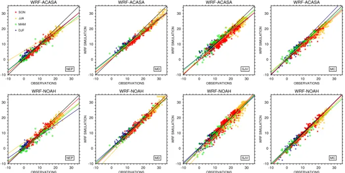
Figure 8 shows scatter plots of simulated monthly surface air temperature from the WRF-ACASA and WRF-NOAH models versus observations, sorted by seasons for the four basins de-fined previously. Each of the points represents a monthly average for one station in the specified basin, and the colors indicate seasons. Least squares regression of the seasonal data shows that both model simulations approach a 1:1 line relationship with the observations. There are some small differences in performances between the two models depending on seasons and locations. This collective analysis of all stations from the four basins shows that although there are some cold biases over the Mojave Desert station, the models generally perform well across the entire basin.
Figure 8. Scatter plots for monthly air temperature simulated by WRF-ACASA (top) and WRF-NOAH
(bottom) for the 4 basins: (Left to right) Northeast Plateau station, Mojave Desert station, San Joaquin Valley station, Mountain County station. Each color simple represents different season: Blue cross = winter (DJF), Green circle = spring (MAM), Yellow triangle = summer (JJA), Red asterisk = fall (SON).
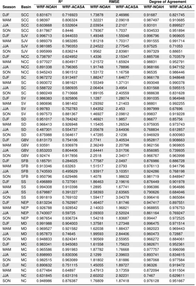
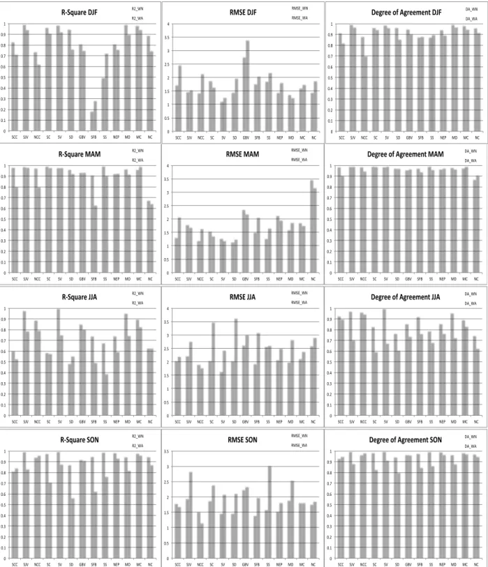
Table 2 and Figure 9 present the statistical analysis of the WRF-ACASA and WRF-NOAH near-surface temperature outputs for each of California’s 13 basins. Statistical values of R-square value, Root Mean Square Error (RMSE), and Degree of Agreement are calculated for each of the basin for each of four seasons. The Coefficient of Determination (or R-square) represents the correlation of the model simulation with the surface observation. The RMSE shows the relative errors of the model simulation against the observation, while the Degree of Agreement is a statis-tical method to assess the agreement between the model simulations with the surface observation.
Table 2. Selected sites from the Air Resources Board meteorological stations network.
R2 RMSE Degree of Agreement
Season Basin WRF-NOAH WRF-ACASA WRF-NOAH WRF-ACASA WRF-NOAH WRF-ACASA
DJF SCC 0.831671 0.716923 1.73878 2.46986 0.91687 0.821745 MAM SCC 0.98397 0.806324 1.32221 2.09018 0.987497 0.910685 JJA SCC 0.603668 0.532604 2.03934 2.2107 0.93101 0.899527 SON SCC 0.817867 0.8446 1.79367 1.7037 0.934533 0.951894 DJF SJV 0.996713 0.944033 1.49348 1.55048 0.996796 0.969605 MAM SJV 0.989379 0.983285 1.81218 1.70317 0.991555 0.991714 JJA SJV 0.981085 0.790353 2.24522 2.77545 0.97525 0.71053 SON SJV 0.995999 0.836214 1.9562 2.83981 0.997329 0.88651 DJF NCC 0.738797 0.624952 1.4336 2.15347 0.885708 0.703579 MAM NCC 0.977027 0.804917 1.21572 1.65924 0.98831 0.952791 JJA NCC 0.891338 0.796365 1.91748 1.78896 0.968166 0.947152 SON NCC 0.945243 0.961512 1.53172 1.16758 0.96535 0.986446 DJF SC 0.967272 0.913497 1.88247 1.64677 0.966178 0.948648 MAM SC 0.993072 0.981621 1.55349 1.37131 0.993048 0.990378 JJA SC 0.588722 0.580935 2.06404 3.4954 0.831568 0.595515 SON SC 0.980249 0.710668 1.89105 2.40559 0.988638 0.831628 DJF SV 0.986383 0.925806 1.1287 1.28074 0.991035 0.964948 MAM SV 0.980696 0.981402 1.29392 1.21403 0.98801 0.992255 JJA SV 0.99783 0.752783 1.64352 2.453 0.997999 0.67696 SON SV 0.997573 0.881367 1.46927 2.09812 0.99837 0.919228 DJF SD 0.951017 0.764242 1.46921 1.9857 0.96677 0.85756 MAM SD 0.966413 0.926948 1.15405 1.26534 0.975935 0.973743 JJA SD 0.487301 0.554737 2.05678 3.64936 0.768834 0.612857 SON SD 0.875988 0.564617 1.47285 2.1236 0.946929 0.800983 DJF GBV 0.813173 0.754106 2.7741 3.40534 0.952817 0.908663 MAM GBV 0.93591 0.936978 2.36249 2.20798 0.962156 0.969805 JJA GBV 0.853203 0.804406 2.64441 3.01706 0.856085 0.739935 SON GBV 0.92474 0.917856 2.2518 2.34017 0.966767 0.963998 DJF SFB 0.185791 0.284025 1.77587 2.0497 0.876986 0.886728 MAM SFB 0.913346 0.63263 1.51517 2.0793 0.976113 0.941796 JJA SFB 0.743593 0.495629 1.93917 3.10351 0.924286 0.768198 SON SFB 0.950796 0.629486 1.4078 1.98632 0.981719 0.848947 DJF SS 0.496889 0.727061 1.86463 2.19616 0.876449 0.901978 MAM SS 0.994308 0.910398 1.2895 1.67741 0.996386 0.964686 JJA SS 0.679887 0.391227 2.58393 2.63565 0.790626 0.684046 SON SS 0.991819 0.769102 1.59417 3.04378 0.996416 0.865084 DJF NEP 0.813234 0.762997 1.46407 1.81746 0.947417 0.897551 MAM NEP 0.926788 0.928542 2.14003 1.96821 0.968855 0.976753 JJA NEP 0.743007 0.59725 2.09303 2.52024 0.861164 0.769247 SON NEP 0.987654 0.936724 1.54218 1.83687 0.99447 0.972525 DJF MD 0.991988 0.904003 1.37581 1.27348 0.996475 0.971514 MAM MD 0.969527 0.921582 1.62038 1.88437 0.982023 0.969443 JJA MD 0.957873 0.74645 1.99593 2.84406 0.960473 0.72887 SON MD 0.948833 0.824341 1.90569 2.55955 0.966272 0.884061 DJF MC 0.983341 0.945083 1.61558 1.75623 0.982671 0.952361 MAM MC 0.965586 0.991983 1.87782 1.76668 0.977757 0.996098 JJA MC 0.898993 0.830306 2.1299 2.39603 0.893741 0.834615 SON MC 0.982515 0.963089 1.81802 1.81886 0.987068 0.977584 DJF NC 0.890632 0.751115 1.45055 1.89727 0.96326 0.919472 MAM NC 0.677484 0.64897 3.47913 3.17359 0.872094 0.911504 JJA NC 0.631845 0.631316 2.60202 2.92231 0.7467 0.629611 SON NC 0.948986 0.876387 1.76809 1.87418 0.976128 0.951667
" " " " " " " " " " " " " " " " " " " " " " " " ) ) " " " " " " " " " " " " " " " " " " " " " " " " % % "" " " " " " " " " " " " " " " " " " " " " " " " " % % % % " " 0" 0.1" 0.2" 0.3" 0.4" 0.5" 0.6" 0.7" 0.8" 0.9" 1" SCC" SJV" NCC" SC" SV" SD" GBV" SFB" SS" NEP" MD" MC" NC" R"Square)MAM) R2_WN" R2_WA" 0" 0.5" 1" 1.5" 2" 2.5" 3" 3.5" 4" SCC" SJV" NCC" SC" SV" SD" GBV" SFB" SS" NEP" MD" MC" NC" RMSE%MAM% RMSE_WN" RMSE_WA" 0" 0.1" 0.2" 0.3" 0.4" 0.5" 0.6" 0.7" 0.8" 0.9" 1" SCC" SJV" NCC" SC" SV" SD" GBV" SFB" SS" NEP" MD" MC" NC" Degree%of%Agreement%MAM% DA_WN" DA_WA" 0" 0.1" 0.2" 0.3" 0.4" 0.5" 0.6" 0.7" 0.8" 0.9" 1" SCC" SJV" NCC" SC" SV" SD" GBV" SFB" SS" NEP" MD" MC" NC" R"Square)JJA) R2_WN" R2_WA" 0" 0.5" 1" 1.5" 2" 2.5" 3" 3.5" 4" SCC" SJV" NCC" SC" SV" SD" GBV" SFB" SS" NEP" MD" MC" NC" RMSE%JJA% RMSE_WN" RMSE_WA" 0" 0.1" 0.2" 0.3" 0.4" 0.5" 0.6" 0.7" 0.8" 0.9" 1" SCC" SJV" NCC" SC" SV" SD" GBV" SFB" SS" NEP" MD" MC" NC" Degree%of%Agreement%JJA% DA_WN" DA_WA" 0" 0.1" 0.2" 0.3" 0.4" 0.5" 0.6" 0.7" 0.8" 0.9" 1" SCC" SJV" NCC" SC" SV" SD" GBV" SFB" SS" NEP" MD" MC" NC" R"Square)SON) R2_WN" R2_WA" 0" 0.5" 1" 1.5" 2" 2.5" 3" 3.5" SCC" SJV" NCC" SC" SV" SD" GBV" SFB" SS" NEP" MD" MC" NC" RMSE%SON% RMSE_WN" RMSE_WA" 0" 0.1" 0.2" 0.3" 0.4" 0.5" 0.6" 0.7" 0.8" 0.9" 1" SCC" SJV" NCC" SC" SV" SD" GBV" SFB" SS" NEP" MD" MC" NC" Degree%of%Agreement%SON% DA_WN" DA_WA" 0" 0.1" 0.2" 0.3" 0.4" 0.5" 0.6" 0.7" 0.8" 0.9" 1" SCC" SJV" NCC" SC" SV" SD" GBV" SFB" SS" NEP" MD" MC" NC" R"Square)DJF) R2_WN" R2_WA" 0" 0.5" 1" 1.5" 2" 2.5" 3" 3.5" 4" SCC" SJV" NCC" SC" SV" SD" GBV" SFB" SS" NEP" MD" MC" NC" RMSE%DJF% RMSE_WN" RMSE_WA" 0" 0.1" 0.2" 0.3" 0.4" 0.5" 0.6" 0.7" 0.8" 0.9" 1" SCC" SJV" NCC" SC" SV" SD" GBV" SFB" SS" NEP" MD" MC" NC" Degree%of%Agreement%DJF% DA_WN" DA_WA"
Figure 9. Statistical analysis of two model simulations versus observed for R-square, Root Mean Square
Error (RMSE), and Degree of Agreement for the four different seasons. Basin: South Central Coast (SCC), San Joaquin Valley (SJV), North Central Coast (NCC), South Coast (SC), Sacramento Valley (SV), San Diego county(SD), Great Basin Valleys(GBV), San Francisco Bay(SFB), Salton Sea (SS), Northeast Plateau (NEP), Mojave Desert (MD), Mountain Counties (MC), North Coast (NC) Season: winter (DJF), spring (MAM), summer (JJA), fall (SON).
Overall, both of the models have a high degree of agreement with all 700 observation stations within the 13 ARB basins during winter, spring, and autumn. The dry summer season is more problematic than the other seasons for both of the models and more so for the WRF-ACASA model over coastal regions such as South Coast, San Diego, and San Francisco basins. This is most noticeable in the RMSE values for WRF-ACASA over the low vegetated regions of Great Basin Valley (GBV), Salton Sea (SS), and San Diego (SD), which increased dramatically during the warm season. While the Degree of Agreement for the San Francisco Basin (SFB) during the wintertime is high with values above 0.8 for both models, the R-square values show that there is little correlation between the model simulations and the surface observations. It could be due to the small range of observation data. Overall, the temperature simulations from both models agree well with the observations with a high Degree of Agreement. Previous examination on a station-by-station basis also reveals that there is a mismatch in vegetation cover between what is in the WRF models and the actual land surface at the station (e.g., the Mountain County station from Table 1). These mismatches introduce errors that are not due to model physics, and they contribute to some of the low R-square and high RMSE values in the collective study.
Figure 10 shows time series of surface dew point temperature over the same four stations (NEP, MD, SJV, MC). The dew point temperature influences land surface interaction with the atmosphere by indicating conditions for condensation. The disparities between the WRF-ACASA and WRF-NOAH models are more distinct in the dew point temperature than in the surface tem-perature: while both models perform well with the surface temperature simulation, the WRF-ACASA model outperforms the WRF-NOAH in simulating the dew point temperature, especially over the San Joaquin station and during May for the Mojave Desert station. This could be be-cause the complex physiological processes in the WRF-ACASA model allow a more accurate simulation of the humidity profile and physiological interactions. Although the vegetation covers over these two regions are sparse, the multilayer canopy structure in the WRF-ACASA model is likely to retain moisture longer within the canopy. These details put the dew point temperature calculated by WRF-ACASA closer to observations than the WRF-NOAH model, which can only account for a single canopy layer.
Both models have difficulty over the Mojave Desert station, where they underestimated the dew point temperature as much as 15◦C during February and November. Similar to the surface
temperature analysis, both models performed best over the Northeast Plateau station with well-matched land cover type ACASA) and simple canopy structure of short grass (WRF-NOAH). In general, the dew point temperature simulations from the WRF-ACASA model match closely with the observations in magnitude and timing.
Figure 10. Time series of dew point model predictions and observations for four stations during February,
Figure 11 presents diurnal patterns of surface dew point temperature for the four seasons. Un-like for the surface air temperature, there is relatively little diurnal variation in the surface dew point temperature throughout the seasons and locations. The simulated dew point temperatures in both WRF-ACASA and WRF-NOAH are functions of surface pressure and surface water va-por mixing ratio. Since the surface pressure does not change dramatically throughout the day, changes in dew point temperature are mainly due to fluctuations in water vapor mixing ratio. Once again, the dry arid and low vegetated Mojave Desert site is problematic for both models.
Figure 11. Mean diurnal dew point temperature trends for the four seasons and the four stations. Top to
bottom: NEP, MD, SJV, MC. Left to right: winter (DJF) spring (MAM), summer (JJA), fall (SON). Compared to the surface temperature,Figure 12 shows that the model simulations on dew point temperature exhibit more scatter than for other observational sets examined thus far, al-though Figure 10 seems to indicate that WRF-ACASA has a better agreement with surface
ob-servations at the MD station. The seasonal patterns for the entire Mojave Desert Basin show that both WRF-ACASA and WRF-NOAH performances are comparatively poor in this sparsely veg-etated region. The choice of land surface model did not affect the model simulation; hence, the problem could be in the atmospheric processes in WRF and not in the land surface processes.
Figure 12. Time series of surface dew point temperature simulated by WRF-ACASA and WRF-NOAH,
with surface observations for four different stations during the months of February, May, August and November 2006.
This could be the result of the assumption of horizontal homogeneity in each of the 8 km x 8 km grid cells used in both WRF-ACASA and WRF-NOAH. A single homogeneous grid cell could be representing several observation stations with different microclimatic conditions. This is especially important when, for example, the shrublands in the Mojave Desert Basin have dif-ferent degrees of canopy openness. Unlike the previous analysis, Figure 12 shows that the WRF-ACASA model underperforms relative to WRF-NOAH over the Northeast Plateau basin.
Figure 13 compares the relative humidity from both WRF-ACASA and WRF-NOAH with the surface observation for four different locations during February, May, August and October of 2006. Except for the Mountain County station, both models fall mostly within the ±1 stan-dard deviation range with the WRF-ACASA model showing somewhat better agreement than the WRF-NOAH model over the Mojave Desert station. The WRF-NOAH model underestimates the relative humidity for Mojave Desert and San Joaquin Valley throughout the year. Although there is a land cover mismatch between the actual station and the model, the higher relative humidity values in the WRF-ACASA simulation compared with WRF-NOAH during the warm season re-inforce that the multi-layer canopy structure and higher order turbulent closure scheme help the vegetation parameterization to simulate the retention of more moisture within the canopy layers.
Figure 13. Time series of surface relative humidity simulated by WRF-ACASA and WRF-NOAH and the
surface observations for four different stations during winter, spring, summer and fall of 2006. The land cover mismatch in the model could lead to overestimation of the relative humidity in areas of low vegetation cover. The high LAI values over Central Valley and the assumption of horizontal homogeneity with one dominant vegetation cover cause the WRF-ACASA model to preserve too much water within the canopy layers during the warm August conditions instead of evaporating the water rapidly. As a result, WRF-ACASA overestimated the daytime relative humidity.
Figure 14 shows a Taylor diagram of monthly mean surface air temperature, dew point tem-perature, relative humidity, wind speed, and solar radiation simulated by WRF-ACASA and WRF-NOAH for all 730 stations in California. The Taylor diagrams for the four different sea-sons shows that simulations from both models agree well with the surface measurement in every
area except for wind speed. The surface air temperature, with high correlations, low RMSEs, and matching variability, is the most accurately simulated variable by both models when compared to the surface observations. While the WRF-NOAH model has a slightly better standard deviation for the air temperature, the WRF-ACASA is slightly more accurate for dew point temperature. Relative humidity, on the other hand, shows low correlation and high root mean square error from both models. These high root mean square errors and poor correlations could be attributed to the models’ assumption of homogenous vegetation and leaf area cover for each grid cell, especially over low vegetated regions (as previously mentioned).
Figure 14. Taylor diagram of monthly mean surface air temperature, dew point temperature, relative
hu-midity, wind speed, and solar radiation for both WRF-ACASA and WRF-NOAH for all ARB stations. WRF-ACASA is represented by blue dots and WRF-NOAH by red dots.
4. CONCLUSIONS
This study compares and evaluates the two different approaches and varying complexity of ACASA and NOAH land surface models embedded in the state-of-art mesoscale model WRF, as they simulate the surface conditions over California on a regional scale. With vast differences in land cover, ecological and climatological conditions, the complex terrain of California provides an ideal region to test and evaluate both models. Analysis of model simulations for 2006 from both WRF-ACASA and WRF-NOAH were compared with surface observations from hundreds of stations from the California Air Resources Board network. While both ACASA and NOAH land surface models use four soil layers for below-ground representation, the WRF-NOAH uses a single-layer “big leaf” to represent the surface layer for all land cover types. In all single-layer models such as NOAH, there is no interaction or mixing within the canopy regardless of the spec-ified vegetation type. In contrast, the ACASA land surface model uses a multi-layer canopy struc-ture that varies according to land cover type. The complex physically based model includes intri-cate surface processes such as canopy structure, turbulent transport and mixing within and above
the canopy and sublayers, and interactions between canopy elements and the atmosphere. Light and precipitation from the atmospheric layers above are intercepted, infiltrated, and reflected within the canopy layers. These along with other meteorological and environmental forcings are drivers of plant physiological responses. In addition, the higher order closure scheme in ACASA allows down- and counter-gradient transport of carbon dioxide, water vapor, heat, and momentum within and above the canopy layers, and interaction with the atmosphere. Through plant evapo-transpiration, photosynthesis, respiration, and roughness length, the surface ecosystem transforms environmental conditions and influences the atmosphere processes above by modifying surface temperature, dew point temperature, and relative humidity. Compared to the WRF-NOAH, which has a simplified surface and ecosystem representation, the WRF-ACASA coupled model presents a detailed picture of the physical and physiological interactions between the land surface and the atmosphere. Compared to 2-meter near surface observations, WRF-ACASA output may be better suited to simulate understory microclimate, as WRF-NOAH’s “big leaf” has no understory.
Comparisons between model simulations and surface observations show that the WRF-ACASA model is able to soundly simulate surface and atmospheric conditions. Its simulation of tempera-ture, dew point temperatempera-ture, and relative humidity agree well with the surface observations over-all. While both WRF-ACASA and WRF-NOAH simulations agree with the surface observations, model performances vary among land surface representations, depending on surface and atmo-sphere conditions. During the cold and wet winter, both models have a high degree of agreement as well as high correlation with the surface observations, in terms of surface temperature, dew point temperature and relative humidity. However, as the season starts to warm up, a temperature bias for WRF-ACASA in certain regions becomes apparent. Maximum daytime temperatures in the WRF-ACASA simulations are systematically lower than the observed daily maximum over low vegetated regions such as the Mojave Desert. This temperature bias is likely due to discrep-ancy in LAI causing excessive evaporative cooling. For the shrubland vegetation with low leaf area index, the leaf area indices for each of the sub-canopy layers are further reduced. The higher order turbulent closure scheme more effectively reflects the energy transport away from the sur-face level to induce heat loss. These thermodynamical processes allow the WRF-ACASA model to describe the prolonged period of cooling in early mornings. As a result, the high daytime tem-perature is underestimated in the multi-layer model.
The analysis of dew point temperature and relative humidity shows that these more detailed physical processes in WRF-ACASA seem to improve the accuracy of dew point temperature and relative humidity simulations compared to the WRF-NOAH model. The process parame-terizations appear to allow the retention of more moisture within the canopy layers as well as the distribution of moisture within and above the canopy. With more complex and detailed canopy and plant physiological process parameterizations, WRF-ACASA represents the ecosystem-atmosphere interactions more realistically than WRF-NOAH.
Overall, when compared to the simple single layer WRF-NOAH model, the WRF-ACASA model has greater model complexity, allowing it to present a more detailed picture of how the atmosphere and ecosystems interact–including ecophysiological activities such as photosynthe-sis and respiration–without decreasing the quality of the output. The physical and physiological
processes in WRF-ACASA highlight the effect of different land surface components and their overall impacts on atmospheric conditions. In addition, the WRF-ACASA model provides oppor-tunities for more study on the topics of ecosystem responses to atmospheric impacts, such as the contribution of irrigation to canopy energy distribution, land use transformations, climate change, and other dynamic and biosphere-atmospheric atmosphere interactions.
Acknowledgements
This work is supported in part by the National Science Foundation under Awards No.ATM-0619139 and EF-1137306. The Joint Program on the Science and Policy of Global Change is funded by a number of federal agencies and a consortium of 40 industrial and foundation sponsors. (For the complete list see http://globalchange.mit.edu/sponsors/current.html). We also thank Dr. Matthias Falk for his inputs on the WRF-ACASA work.
5. REFERENCES
Borge, R., V. Alexandrov, J. Jos´e del Vas, J. Lumbreras and E. Rodr´ıguez, 2008: A comprehen-sive sensitivity analysis of the WRF model for air quality applications over the Iberian Penin-sula. Atmos. Environ.,42(37): 8560–8574.
Chen, F. and R. Avissar, 1994: The impact of land-surface wetness heterogeneity on mesoscale heat fluxes. J. Appl. Meteor.,33(11): 1323–1340.
Chen, F. and J. Dudhia, 2001a: Coupling an advanced land surface-hydrology model with the Penn State-NCAR MM5 modeling system. Part I: Model implementation and sensitivity. Mon. Wea. Rev.,129(4): 569–585.
Chen, F. and J. Dudhia, 2001b: Coupling an advanced land surface-hydrology model with the Penn State-NCAR MM5 modeling system. Part II: Preliminary model validation. Mon. Wea. Rev.,129(4): 587–604.
Chen, S. and J. Dudhia, 2000: Annual report: WRF physics. Air Force Weather Agency. Chen, S. and W. Sun, 2002: A one-dimensional time dependent cloud model. J. Meteor. Soc.
Japan,80(1): 99–118.
de Wit, M., 1999: Modelling nutrient fluxes from source to river load: a macroscopic analysis applied to the Rhine and Elbe basins. Hydrobiologia,410: 123–130.
Denmead, O. and E. Bradley, 1985: Flux-gradient relationships in a forest canopy. The forest-atmosphere interaction: proceedings of the forest environmental measurements conference, pp. 421–442.
Dickinson, R., A. Henderson-Sellers and P. Kennedy, 1993: Biosphere-Atmosphere Transfer Scheme (BATS) Version 1e as coupled to the NCAR community model. NCAR Tech. Note NCAR/TN-387+ STR,72.
Duan, Q., S. Sorooshian and V. Gupta, 1992: Effective and efficient global optimization for con-ceptual rainfall-runoff models. Water Resour. Res.,28(4): 1015–1031.
Dudhia, J., 1989: Numerical study of convection observed during the winter monsoon experiment using a mesoscale two-dimensional model. J. Atmos. Sci.,46(20): 3077–3107.
Etchevers, P., E. Martin, R. Brown, C. Fierz, Y. Lejeune, E. Bazile, A. Boone, Y. Dai, R. Essery, A. Fernandez et al., 2004: Validation of the energy budget of an alpine snowpack simulated by several snow models (SnowMIP project). Ann. Glaciol.,38(1): 150–158.
Gao, W., R. Shaw and K. Paw U, 1989: Observation of organized structure in turbulent flow within and above a forest canopy. Bound.Lay. Meteorol.,47(1): 349–377.
Holtslag, A. and M. Ek, 1996: Simulation of surface flux and boundary layer development over the pine forest in HAPEX-MOBILHY. J. Appl. Meteor.,35(2).
Hong, S. and H. Pan, 1996: Nonlocal boundary layer vertical diffusion in a medium-range fore-cast model. Mon. Wea. Rev.,124(10): 2322–2339.
Houborg, R. and H. Soegaard, 2004: Regional simulation of ecosystem CO2and water vapor ex-change for agricultural land using NOAA AVHRR and Terra MODIS satellite data. Applica-tion to Zealand, Denmark. Remote Sens. Environ.,93(1): 150–167.
Jarvis, P., 1976: The interpretation of the variations in leaf water potential and stomatal conduc-tance found in canopies in the field. Philos. Trans. Roy. Soc. London A,273(927): 593–610. Jetten, V., A. de Roo and D. Favis-Mortlock, 1999: Evaluation of field-scale and catchment-scale
soil erosion models. Catena,37(3): 521–541.
Mahrt, L. and M. Ek, 1984: The influence of atmospheric stability on potential evaporation. Col-lections.
Marras, S., D. Spano, C. Sirca, P. Duce, R. Snyder, R. Pyles and K. Paw U, 2008: Advanced-Canopy-Atmosphere-Soil Algorithm (ACASA model) for estimating mass and energy fluxes. Ital. J. Agron.,3(3 Suppl.): 793–794.
Marras, S., R. Pyles, C. Sirca, K. Paw U, R. Snyder, P. Duce and D. Spano, 2011: Evaluation of the Advanced Canopy–Atmosphere–Soil Algorithm (ACASA) model performance over Mediterranean maquis ecosystem. Agric. For. Meteor.,151(6): 730–745.
Meyers, T. and K. Paw U, 1986: Testing of a Higher-Order Closure Model for Modeling Airflow within and above Plant Canopies. Bound.Lay. Meteorol.,37: 297–311.
Meyers, T. and K. Paw U, 1987: Modelling the plant canopy micrometeorology with higher-order closure principles. Agric. For. Meteor.,41(1): 143–163.
Miglietta, M. and R. Rotunno, 2005: Simulations of moist nearly neutral flow over a ridge. J. Atmos. Sci.,62(5): 1410–1427.
Mintz, Y., 1981: A brief review of the present status of global precipitation estimates. Report of the Workshop on Precipitation Measurements from Space.