The deterioration in heat transfer to fluids at super-critical pressure and high heat fluxes

R. NO t. .. o '* 4.-i

ENGINEERING PROJECTS LABORATORY NGINEERING PROJECTS LABORATOR'

4GINEERING PROJECTS LABORATO' IINEERING PROJECTS LABORAT'

~NEERING PROJECTS LABORK 'EERING PROJECTS LABOR

ERING PROJECTS LABO' RING PROJECTS LAB'

ING PROJECTS LA iG PROJECTS L

1 PROJECTS PROJECT.

THE DETERIORATION IN HEAT TRANSFER

TO FLUIDS AT SUPER-CRITICAL PRESSURE

AND HIGH HEAT FLUXES

Bharat S. Shiralkar

Peter Griffith

Report No. 70332-51

Department of Mechanical

Engineering

Engineering Projects Laboratory

Massachusetts Institute of

Technology

THE DETERIORATION IN HEAT TRANSFER TO FLUIDS AT SUPER-CRITICAL PRESSURE AND HIGH HEAT FLUXES

by Bharat S. Peter Shiralkar Griffith Sponsored by

American Electric Power Service Corp.

March 1, 1968

Engineering Projects Laboratory Department of Mechanical Engineering

Massachusetts Institute of Technology Cambridge, Massachusetts

TABLE OF CONTENTS

1. INTRODUCTION 1

2. SCOPE OF PRESENT INVESTIGATION 3

3. EXPERIMENTAL EVIDENCE OF PREVIOUS

INVESTIGATORS 4

4. PROPERTIES AND THERMODYNAMICS NEAR THE

CRITICAL POINT 7

5. THEORETICAL APPROACH 9

1. Introduction 9

2. Basic Equations 9

3. Expressions for the Eddy Diffusivity 16

4. Method of Solution 20

5. Results 21

6. Simplified Physical Model 27

7. Safe Versus Unsafe Plot for Steam 35

6. EXPERIMENTAL APPROACH 37

1. Introduction 37

2. Description of Apparatus 37

3. Capabilities and Measurements 39

4. Experimental Results 40

5. Factors Affecting Deterioration 43

6. Comparison with Computed Wall Temperature Versus

Bulk Enthalpy 46

7. Experimental Safe Versus Unsafe Plot for CO2 46 8. Comparison Between Upflow and Downflow 49

7. FUTURE WORK 55

8. CONCLUSIONS 56

LIST OF FIGURES

Fig. Page

1. Variation of the Heat Transfer Coefficient with

Heat Flux in the Critical Region (From Ref. 33) 2 2. Deteriorated Heat Transfer Region (Shitsman) 5

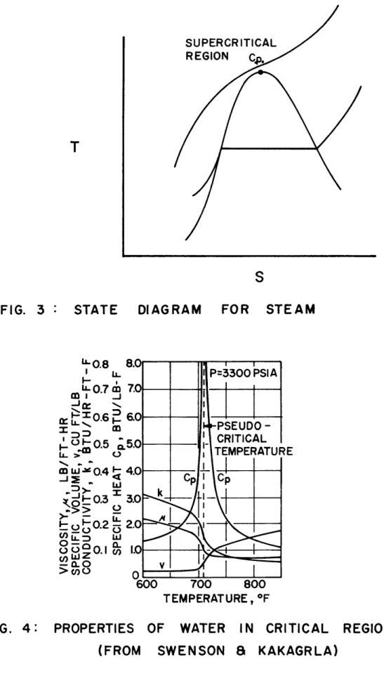
3. State Diagram for Steam 8

4. Properties of Water in Critical Region (From Swenson

and Kakagrla) 8

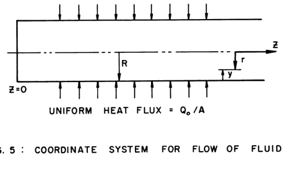
5. Coordinate System for Flow of Fluid 10

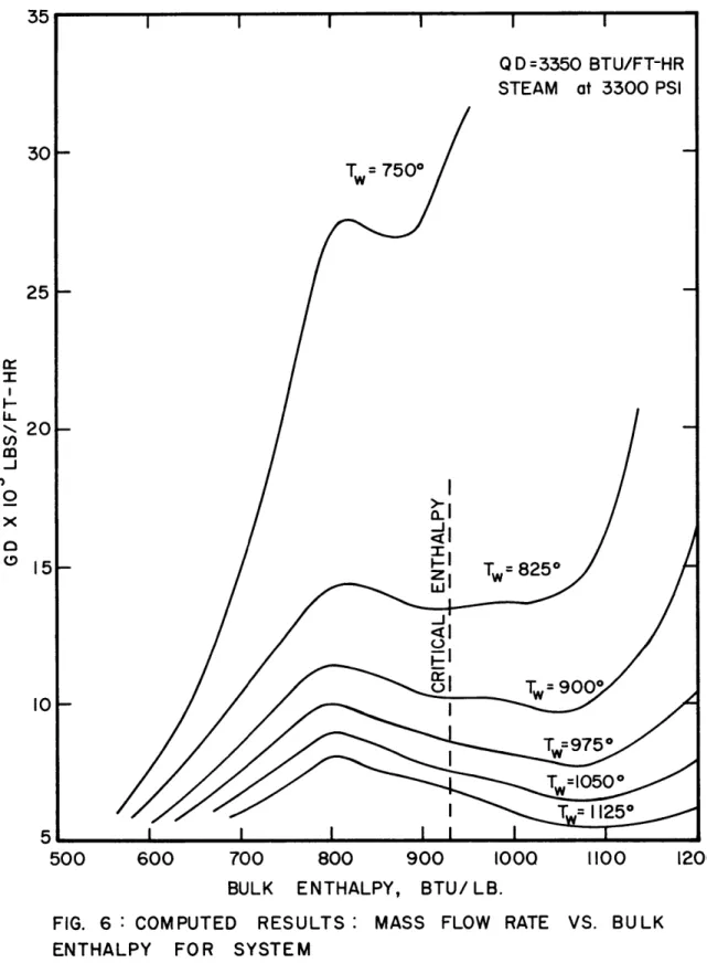
6. Computed Results: Mass Flow Rate Versus Bulk

Enthalpy for System 22

7. Computed Results: Mass Flow Rate Versus Bulk

Enthalpy for System 23

8. Computed Results: Mass Flow Rate Versus Bulk Enthalpy

for System 24

9. Computed Results: Mass Flow Rate Versus Bulk Enthalpy

for System 25

10. Deteriorated Heat Transfer Region (Shitsman) 26 11. Computed Results: Constant Shear Stress Lines 28 12. Variation of Shear Stress with Heat Flux 29

13. Computed Velocity Profiles 30

14. Computed Temperature Profiles 31

15. Radial Locus of Tc in a Typically Deteriorated Region 32 16. Physical Explanation of Heat Transfer Variation 34 17. Computed Safe Versus Unsafe Plot for System 36

18. Schematic Drawing of Experimental Loop 38

19. Data Print-Out 41

20. Experimental Results for CO 2 at 1100 Psi 42 21. Experimental Results Showing Effect of Inlet Enthalpy

on the Temperature Versus Length Profile 44 22. Experimental Results Showing Effect of Tube Vibration 45 23. Experimental Results for CO at 1150 Psi 47 24. Comparison Between Computed and Experimental

LIST OF FIGURES (Continued)

Fig. Page

25. Experimental Safe Versus Unsafe Plot for CO2 at 1100

Psi 50

26. Experimental Safe Versus Unsafe Plot for CO 2 at 1150

Psi 51

27. Comparison Between Computed and Experimental Safe

Versus Unsafe Plots 52

28. Experimental Results for Downflow 53

NOMENCLATURE

Cp local specific heat at constant pressure, ( BTU/lb0 F) Cp0 reference value of specific heat, ( BTU/lb

0 _F) D diameter of tube, (ft.)

2

g acceleration due to gravity, (ft/hr.

)

G mass flow rate, (lbs/ft 2-hr.)

Gr Grashof Number = (pb - o o 9 23o 3

hi heat transfer coefficient, (BTU/ft - F-hr) h local enthalpy, (BTU/lbs.)

H bulk mean enthalpy at a cross-section (BTU/lb) k local conductivity, (BT U/ft-hr -'I

k0 reference value of thermal conductivity, (BTU/ft-hr-0 F)

K constant = 0. 36

L length along tube, (ft.)

n constant = 0. 124

Nu Nusselt Number = hD/k

Numac MacAdams' Nusselt Number 0.8 04

p pressure, (lbs/ft. ) Pr Prandtl Number = Cpm/k

Pro Cpj 0o/k₀ 2

q local heat flux, (BTU/ft2 -hr) Q0/A wall heat flux (BTU/ft -hr) R radius of tube, (ft)

Re Reynolds Number = GD/

T temperature (OF)

U local velocity, axial, (ft/hr)

U + U/ w

U

dU/r97/p

V local radial velocity, (ft/hr) y distance from wall, (ft)

Y nondimensionalized distance = y/R

+~~

~~

+w Y w-WA

y0 o ri/p/

dy

Z axial coordinate, (ft)

NOMENCLATURE (Continued) local radius, (ft)

eddy diffusivity of heat, (ft 2/hr)

eddy diffusivity of momentum, (ft

/hr)

local viscosity, (lbs/ft-hr)

reference value of viscosity, (lbs/ft-hr) density, (lbs/ft3₎

reference value of density, (lbs/ft 3

2

wall shear stress (lbs/ft-hr ) 2

local shear stress (lbs/ft-hr

)

Superscripts and Subscripts used

refers to bulk mean quantity

refers to quantity at wall or wall temperature refers to a reference value of quantity

nondimensionalized quantity Eh m o p p0 o 0

1. INTRODUCTION

Several supercritical steam generators in the American Electric Power system have shown evidence of tube overheat in the lower furnance at the point where the water bulk temperature is about 670 0F. The

evi-dence is of two kinds. First thermal fatigue has occurred and caused tube failures long before a failure of any kindwas to be expected. Second, pairs of cordal thermocouples have shown very high wall temperatures and,

extrapolating back to the inside of the tube, evidence reduced inside heat transfer coefficients. It was suspected that a possible cause of the high tube temperature was a supercritical "burnout". The primary purpose of this investigation is to determine the cause and conditions leading to a

supercritical "burnout" such as might occur in a supercritical steam generator.

Before focusing on this aspect of the problem it is worthwhile to mention several other possible causes for the high tube wall temperatures which have been observed. In this context high means higher than the design temperature. Let us just list these possibilities.

1. Scale inside the boiler tubes.

2. Hot spot factors in the design procedure which are too low. 3. Higher heat transfer from the combustion gases than expected. Better design procedures or better control of the water purity might be sufficient to cause the problem to disappear without changing the water flow conditions inside the tube.

Because the three factors which are listed above are really rather vague, it appeared that the most promising approach is to eliminate the excessive temperatures inside the tube at supercritical pressure is to

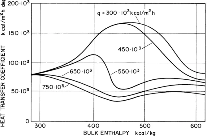
eliminate the "burnout". Therefore, only the burnout aspect of the pro-blem has been studied here. The undesirable behavior of the Nusselt number, which is of interest, is indicated in Fig. 1. In particular we want to find out when the supercritical Nusselt number is less than one would expect from the affects of simple property variations alone.

200

103 c

E

N% 7F3 15 0I5O1O

100.103

50

103

0

300

400

500

BULK ENTHALPY

kcal/kg

600

FIG. I. VARIATION OF THE HEAT TRANSFER COEFFICIENT WITH

HEAT FLUX IN THE CRITICAL REGION (FROM REF 33)

q = 300 -1O3 k cal/m

2h

450-103-650-103

\.550-103

2. SCOPE OF PRESENT INVESTIGATION

An experimental and theoretical investigation of the heat transfer at high heat fluxes was undertaken at the Heat Transfer Laboratory at M. I. T. The experimental program was performed with CO2 as the work-ing fluid because of its convenient critical range.

In general, the methods available for analysis of turbulent flows are either based on the integration of the transport equations with

engineering assumptions for the eddy diffusivities of momentum and heat or on integral methods. Often, a Reynolds analogy is useful for correlating the friction factor to the Stanton number.

Another method, frequently used, is to attempt to modify the normal correlations for constant properties by evaluating the dimensionless groups at some reference temperature usually somewhere between the wall and bulk temperatures. In the present instance, it is doubtful whether a reference temperature taken as a fixed linear combination of the wall temperature and bulk temperature will prove useful, because of the nonlinear behavior

of the heat transfer coefficient with heat flux.

The method most intensively used in this report is based on the integration of the radial transport differential equations.

-3. EXPERIMENTAL EVIDENCE OF PREVIOUS INVESTIGATORS

The phenomenon of deteriorated heat transfer at high heat fluxes when transferring heat to a fluid at supercritical pressure has been

ob-served with several fluids by various investigators. The most detailed work is that of Shitsman (1)A for water, Deterioration has also been reported by Vikrev and Lokshin (2), Shitsman, Miropolskiy and Picus (3), Swenson and Kakarala (4) for water, Powell (5) for oxygen, Szetela (6) in hydrogen and McCarthy (7) in nitrogen tetroxide.

The conditions under which the deterioration was observed to occur are:

1. The wall temperature must be above and the bulk temperature below the psuedocritical temperature.

2. The heat flux must be above a certain value, dependent on the flow rate and pressure.

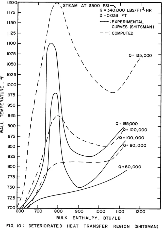
Figure 2 shows a typically deteriorated region in water from the data of Shitsman (1). The dotted line shows the wall temperature at a flux of 132, 000 BTU/ft. -hr. as predicted using the MacAdams correlation (NU = 0.023 (Pr)0 . 4(Re)0. , in which the bulk temperature is used to evaluate the properties and serves as a reference.

Investigations have shown that the amount of deterioration depends on the inlet enthalpy and pressure (1), and on the orientation of the tube. In particular, the data of Lokshin et al (2) indicates that the deterioration in horizontal tubes is less than and not as sharp as that occuring in

vertical tubes foi- a comparable heat flux. Also, the deterioration in larger tubes has been found to be worse (8).

Similar burnout conditions have been reported in hydrogen and oxygen. In these cases, the rise in temperature has been found to be of even larger magnitude than in water.

1200

1175

STEAM

AT 3300 PSI

1150

G

=

340,000 LBS/FT

2

-HR

D = 0.033 FT

1125

_-

_EXPERIMENTAL

1100

CURVES

(SHITSMAN)

- - MACADAM'S

1075

-

CORRELATION

(BULK

PROPERTIES)

1050-1025

-1000

-975

-0

.

950

-925

-

900-875

-850

-

S825725

-700

600

700

800

900

1000

1100

1200

BULK ENTHALPY, BTU/LB

HEAT TRANSFER REGION (SHITSMAN)

Though a number of experiments have been done with CO2 as the working fluid (9, 10, 11, 12, and 13) deterioration has not been observed with CO2. However, most of these investigations were at relatively small heat fluxes.

4. PROPERTIES AND THERMODYNAMICS NEAR THE CRITICAL POINT

The reason for the nonlinear behavior of the heat-transfer coefficient with the heat flux is the strong dependence of the properties of the fluid on the temperature in the neighborhood of the critical temperature.

Figure 3 shows the state diagram for CO2. where a constant pres-sure line at subcritical prespres-sure is represented by 1-1, and at the critical pressure the constant pressure line is represented by 2-2. Assuming thermodynamic equilibrium to exist, an equation for the critical isotherm may be derived by satisfying the conditions for liquid and vapour to co-exist in stable equilibrium with a plane interface in the limiting case. Thus, above the critical pressure, the fluid undergoes no phase transition as it is raised in temperature from below critical to above critical temperature. For the purposes of theoretical analysis in this report, the fluid has been treated on a single phase fluid.

At the critical temperature, the transport properties, viscosity and conductivity, as well as the density, fall sharply, while the specific heat peaks to a high value. Properties of various fluids in the critical region have been investigated and are fairly well known. The properties of water in the critical region were determined by Novak (13), Novak and Grosh (19)

etc., and the properties of carbon dioxide were determined by Michels et al (15, 16, 17, 18, and 19), Clark (20), Keesom (21), Tzederberg (22) etc.

Figure 4 shows the variation of properties for water at 3300 psi. There has been some controversy regarding the measurement of the thermal conduc-tivity at the critical point. Some investigations report' a peak in conducconduc-tivity at the critical temperature. This has usually been discounted as error in

measurement due to thermal convection due to large density differences at the critical point. In this report, the conductivity is assumed to decrease

FIG. 3

STATE

DIAGRAM

**0. 8

LL 0.7 cD I

0.6

a:

LL

.wz0.15

L> mD w -w 0.4 -jO.3 0ot.2

coo

SUPERCRITICAL REGION

Cn.-FOR

STEAM

TEMPERATURE , *F

FIG. 4:

PROPERTIES

(FROM

OF

WATER

IN CRITICAL

SWENSON

8

KAKAGRLA)

REGION

5. THEORETICAL APPROACH

1. Introduction

The problem was treated as that of heat transfer to a single phase, turbulent flow with variable properties in order to obtain a theoretical

solution. The method used was to solve the simultaneous differential equations governing the momentum and energy balance in the fluid, after making numerous simplifications. The equations were then solved in

difference form on the IBM 360 computer at the M.I. T. Computation Center. 2. Basic Equations

The equations governing the flow of a fluid through a constant area pipe, in the steady state, and assuming axial symmetry are:

Continuity 8(pU) +

a

(pYV) = 0 ₍₁₎

8z

'Y (3Y

Momentum .. + - +

--

-. = 0 (2) y -y dZ Energy

p Cp U --

+

--

= -

-

(yq)

(3)

az

ay

/Y

'Y a

where y = local radius

Z = axial coordinate (Fig. 5) U = local axial velocity V = local radial velocity T = local temperature

-r = local wall shear stress

dp/dZ = pressure gradient in the axial direction

q = local heat flux

p = local density

Cp = local specific heat at constant pressure

This formulation assumes that the momentum terms are small compared to the sheer stress and that there is no radial pressure drop, and neglects axial conduction. Also, the momentum equation does not take into account the gravitational term. Hsu (23) has shown that for vertical flow, the effects

of free convection are slight in the critical region as long as the Grashoff number is smaller than 10~

Furthermore, the transport equations

q= -(k

+

pCp E h)

aT

(4) ay -= (j±+ p e) 8U(5) where k = conductivity Ii = viscosity

E h' and E m are the eddy diffusivities of heat and momentum

must be substituted into the Eqs. (2) and (3) and the resulting equations solved for U, V and T.

This system of two-dimensional equations can be solved with boundary values specifying the fully developed velocity and temperature profiles at the beginning and end of a long section, together with the

boundary conditions U = 0, V = 0 at y = R.

A solution of this type was first attempted with some degree of success, but was given up in favor of a simpler solution which required less time on the computer.

Great simplification is achieved by treating the problem as one of fully developed flow and using only a gross continuity condition over the cross-section.

R

UNIFORM

HEAT FLUX

FIG. 5

:

COORDINATE

SYSTEM

FOR

FLOW OF

FLUID

r

y

= 0 . /A

I

RI

The simplified system of equations becomes: Continuity (6) G = Of2ypUdy -rR2 Momentum -r - = Y ₍₇₎ Energy Y U8T yp Cp =T

SZ

Uyp Cp --_{I Z bulk} 8 h - PU8 ZI bulk - (yq) 8y

G = mass flow rate/area T₀ = wall shear stress

R = radius of tube Introducing, ah OZ _bulk 2Q 0 A GR where

Q0/A = wall heat flux/area, the energy equation becomes where

Q

2yp U

---8

A

. (yq) =

ay

GR

(9)

which gives the variation of q along the radius. A still simpler form can be used for the variation of q by noticing that near the wall q = (Q0/A), and at the center q = 0. In the central turbulent core, the variation of q does not influence the results by much. Thus a linear variation in q may be pre-scribed q Q 0 A (10) R

Both forms of Eqs. (9) and (10) were tried and the results were found to differ very slightly, hence the simpler form of Eq. (10) was later adopted.

The final simplified equation now becomes

_ - R-y R R _ y _ R R G = --- f-R f-R R2

where y = distance from equations

ZpU(R-y) dy

the wall = R - y together with the transport

dU T =

( + PE M

dy q = - (k + pCpEh) dT dy 0r 0 q Q 0 A -y R

which yield r (R -y) _dU R dy Q

-

(R -y)

A dT q= - (k + p Cp E h) -- (12). R dy

which can be solved simultaneously for U, T with the boundary conditions.

y = 0, U = 0, T = T_wall

with prescribed wall shear stress T 0, and heat flux Q0/A, and when the eddy diffusivities are known.

The mass flow rate and bulk enthalpy at a section are then obtained as: R

G

2~-

of

2(R-y)Updy

(13)

R2 R -= o 2(R-y)Uphdy (14) R2G 0

A rudimentary nondimensionalization may be achieved by using reference values of the properties and reference temperature and a reference enthalpy.

(1- Y + + + Em dU+ (15)

Qo+ (1- Y) =k+ 1

G + = 2f

(1I

H +

+ p+ Cp+ Pr

0

h vj + U+ Y)

Of

dT+ dy dY + U+ + h+ dY

where + indicates nondimensionalized values, o indicates reference values y y/R

+ = p

/p

₌

= po/p 0 = reference kinematic viscosity

Q k+ Cp+ = _Up 0

/RTr

₀ = RQ0/A/T 0 k0 = _k/k0 = Cp/Cpo

Pr0 = Cp9 9p/k0 = reference Prandtl number T+ = T/T0 G + =GR/O + 2 2 T+ ₀ =T R _o zp lo H+ = H/h ₀ h+ = h/h0

with the boundary conditions

y = 0, U 0,

T+ = T+

_wall

(16)

(17)

This formulation has the advantage of eliminating the radius of the tube R as a separate variable,. and reduces the input variables to T+wall' o ' 0+ and the output variables to G

+,

H +, T +, U+ for a

particular pressure.

It should be mentioned that radial integration of this sort has been done before, particularly by Deissler (24). However, it is felt that the type of solution obtained, in terms of quantities nondimensionalized with respect to the shear stress, does not represent the complete solution since the shear stress is not known and cannot be calculated with a constant pro-perty correlation. The present solution extends the procedure used by Deissler by solving for the shear stress with the additional constraint by Eqs. (13) or (17).

3. Expressions for the Eddy Diffusivity

In order to solve for the velocity and temperature profiles from the preceding equations, expressions for the eddy diffusivities of momentum and heat transfer are required. First of all, it is assumed that the two are

equal. Investigations in the past have shown that this is a good assumption when the Prandtl number is not significantly different from unity, and that

in this range the ratio of the diffusivities is a weak function of Prandtl number (25).

The best known forms for the eddy diffusivity are due to Deissler (26), van Driest (27) and Spalding (28). Of these, Deissler's is probably the

easiest to use and van Driest's the most accurate (29).

For constant property flow, Deissler's expression is

E =nUy y+ < 26 2 3 _ k - (dUdy) (dU__dy) y > 26 d2U 2 dy 2

-o

+ Po

y - _ y, n = 0. 109, k = 0. 36

The velocity profiles generated with this expression, match the experimental profiles closely.

For variable property flow, in order to take into account the effect of the local kinematic viscosity, Deissler (24) has suggested the use of the following expres sion:

e = n Uy(l-e -n2Uyp/

= k2(dU/dy)3/(dzu/dy 2 )2

y ' < 26

y+ > 26

where p, are the local properties andpo/p9 are the properties evaluated at the wall temperature.

In the central region y +> 26, it is easier to use Prandtl's expression for diffusivity

2 2

C = k y dU/dy

k = 0.36

Thus, the formulation for the eddy diffusivity becomes (as used by Hsu (23)) Deissle r, E = n U-n2U+ + p ₀ k2 o +2 dU+ = - _y Ro dy+ y+ < 26 y > 26 where

Since this formulation involves the use of y +, U+ based nn the properties at the wall temperature, an improvement has been suggested

by Goldmann (30) in which y +, U+ are replaced by y , U++

where + + y _o d y dy, o fp U ++ dU U -_ 0 P so that the expressions for the diffusivity become

Goldmann:

2fU++y++

.-

1-exp (-n2U++Y++

k 2 p ++2 dU++

P dy++

y ++< 26

++ y y>26

The diffusivities suggested by Deissler, Goldmann and van Driest were tried and found to yield the same type of results, with differences in wall to center line temperatures of less than 10 per cent. Goldmann's scheme has been employed for the bulk of the work since it is more appealing than Deissler's on a physical basis for the reason that it uses an integrated value of the Reynolds number y+ to determine the transition from the viscous to the turbulent region, rather than y+ based on the properties at wall tempera-ture.

Several modifications have been suggested in the form of the eddy diffusivity to take into account the presence of large density gradients in the critical region, which tend to promote greater mixing Hsu (23) and Hall (9) suggested multiplying the conventional diffusivity by amplification factors, i. e.

Hsu:

C conventional (1 + A)

Hall: E E conventional x C

[1

dp p dT

Etl

dpi

p dT Tstandard

where B is a constant to be determined experimentally.

These enhanced diffusivity models suffer from the defect that they lead to enormous diffusivities very close to the wall when the critical temperature is in the vicinity of the wall and yield very large heat transfer

rates, irrespective of the magnitude of the heat flux, which is clearly contrary to experiment.

Thus, the diffusivity form suggested by Goldmann has been adopted where ++ y - 0-p dy = Y ++ 0

f

dY U U+

f

dU

+

p

+ d

U

O '/ TO

in terms of previously nondimensionalized quantities where 2 + 0 R po P 0 2 14

U

+

11 0

o

RT

4. Method of Solution

The solution consists in numerically solving the Eqs. (11) and (12) (using the expressions for eddy diffusivity in the previous section) for a prescribed heat flux Q0/A, shear stress and wall temperature and then evaluating the mass flow rate and bulk enthalpy from the integrals in Eqs. (13) and (14). The method used was an explicit finite forward difference procedure, starting at the wall and proceeding inwards to the center of the tube. Because of the large amount of calculation involved in computing the profiles for various wall temperatures and wall shear stresses, this

method was preferred as being the quickest over a formal relaxation pro-cedure, though it is less accruate. By using a first order difference pro... cedure which yields a positive error in the bulk velocity and temperature drop and a second order procedure, which yields a negative error, bounds can be placed onthe solution. For constant properties, the solution checks with known results to within 2 per cent.

Thus, the essentials of the solution can be tabulated in the following way:

Q /A T wr T U G H

50,000 800 2x 107 800 0 4 x 105 685

798 200

5. Results

The bulk of the results are presented in the form G+ versus H+

for different wall temperatures and heat flux parameter Q . In order to feed in the properties without reducing them by division by standard

quantities, it was found convenient to designate the value of unity to all reference quantities

p = f(T) can be represented numerically by

p/p 0 = f(T/T ) etc.

G+ = GR/11L represents the numerical value GR

Qo+

= PQ0

/A)R/T

0k0 represents the numerical value QQ/A x R

+ 2 2 2

0 = ToR p

/OA

represents the numerical value T- R

Figures 6, 7, 8 and 9 are plots of GD versus H for different wall tempera-tures for three different values of the heat flux parameter QD = 3300, 5000, 15000, 25000 BTU/ft. -hr. The GD range in each plot is such that it shows the region of interest, where hot spots are likely to occur. The peak and

dip in the isotherms correspond to the maximum flow rate (in the pre-critical enthalpy region) and the minimum flow rate possible at that temperature, respectively. These represent the point of the maximum temperature for the first flow and the minimum temperature for the second flow rate respectively.

In order to use these plots for a particular problem, it is necessary to make a crossplot of wall temperature versus bulk enthalpy for a constant flow rate. Figure 10 shows crossplots made for G = 340, 000 lbs/ft. hr. for three heat fluxes, Q = 80, 000, 100, 000, and 132, 000 BTU/ft2-hr for a tube of diameter 1/30 ft. in order to compare these results with the experimental re-sults of Shitsman(l). This plot corresponds to the variation of wall temperature along the length of a tube with uniform heat input. It is seen that the

cal-culations predict a marked deterioration in heat transfer at about the same heat flux observed experimentally. It is also evident that the predictions are somewhat high in the region beyond the peak. This is probably due to the fact that there is additional mixing in this region of large density

gradients in the core, which has not been taken into account in the calcula-tions. Also this is the region where the fully developed profile assumptions

600

700

800

900

1000

1100

BULK

ENTHALPY,

BTU/LB.

FIG. 6 : COMPUTED

RESULTS: MASS FLOW RATE

ENTHALPY

FOR SYSTEM

VS. BULK

30

25

-:

-20

x

10

500

1200

850

20,000-925

15,000

-1000

105

10,000CRITICAL

_10,000

1 150

-ENTH

AL PY

500

600

700

800

900

1000

1100

1200

1300

1400

H ,BTU/

LB

60 -

₁₀₀₀

65-cn

₁₂₅₀

41300 0 252

35

30 CRITICAL ENTHALPY 500 600 700 800 900 1000 1100 1200 1300 1400 1500

BULK ENTHALPY , H, BTU/LB

QD= 25,000 STEAM AT 3300 PSI 200 190 180 -170 -160 ~0 r 150 -140 -130 -U'l m0000, 120 -- 110 -/s0 ( 100 - -90 - O 800 80 --e 70 60 CRITICAL of 50 1 1 1ENTHALP IY \' 0 \ 01 50 500 600 700 800 900 1000 1100 1200 1300 1400 1500 H BTU /LB

STEAM AT 3300 PSI-, I 2

G

=

340,000

LBS/FT- HR

D =

0.033 FT

-- EXPERIMENTAL

CURVES (SHITSMAN)

- -: COMPUTED

1175

1150

1125

1100

1075

1050

1025

1000

975

950

Q

=

135,000

/Q=

100.000

100,000

=

80,000

000

BULK

ENTHALPY,

1200

BTU/LB

FIG. 10: DETERIORATED

HEAT

TRANSFER

REGION

_(SHITSMAN)

Q=

135,000

I

I

I

I

I

I

I

I

I

925

-

900-875

850

825

800

775

750

725

/

700

600

700

800

900

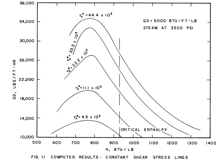
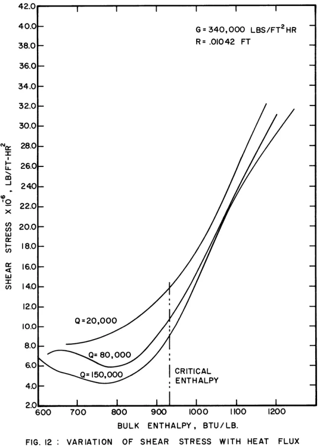
Since the variation of shear stress along the length is an important part of the solution, a sample plot of GD versus enthalpy is shown in

Fig, 11 for various values of -r0 . A crossplot of shear stress versus enthalpy (Fig. 12) shows that the shear stress dips before rising to a higher value corresponding to the gaseous state. An examination of

the effect of heat flux shown that the dip gets more pronounced at a higher value of the heat flux.

Figures 13, and 14 show typical velocity and temperature profiles at different sections of the tube, corresponding to the deteriorated region and regions in the liquid and vapors regimes, away fromthe critical point. The temperature drop in the region close to the wall is proportionately lar-ger in the deteriorated region. An explanation, sometimes suggested for the deterioration phenomenon, is that 're-laminarization' of the boundary layer takes place. Though this is confirmed by this investigation to the ex-tent that there is a drop in the shear stress, the velocity profiles do not tend towards the conventional laminar velocity profiles. The drop in shear stress is largely due to the drop in density and viscosity near the wall, without an appreciable increase in the core velocity.

The locus of the critical temperature is of some interest, for example, in the formulation of integral methods of solution. Figure 15 shows that the locus is 'flatter' than for a constant property flow, i. e., the critical temperature persists longer near the wall.

6. Simplified Physical Model

It is possible to postulate a simple physical model to explain the deterioration phenomenon, based on the evidence of the computed results.

If the equations governing the flow are examined, (1-Y) q0 = -p(k/p Cp + E h)dh/dY, (1 -Y)r 0 = p (1±/p + e m)dU/dY. it is evident that the velocity profiles and enthalpy profiles will be identical if the molecular Prandtl number Cp1 /k and the turbulent Prandtl number e m/E h) are both unity.

Since the assumption that E m = E h has been made, and the Prandtl number Cpp /k does not differ largely from unity except in small regions, it should be expected that the relation

-38,000

34,000

30,000

26,000

22,000

18,000

14,000

10,000

L

500

600

700

800

900

1000

H, BTU/

LB

1100

1200

1300

1400

42.1

G=340,000

LBS/FT

2HR

R = .01042

FT

36.0

34.0-

32.0-

30.0-Noa:

28.0

u

26.0

-

240-to

22.0-x

o'

20.0-w

18.0-

16.0-w

u

14.0-

12.0-10.0-

Q=20,000

8.0-Q= 80, 000

Q=150,000

CRITICAL

ENTHALPY

4.0-600

700

800

900

1000

1100

1200

BULK ENTHALPY,

BTU/LB.

1140,.

102

F

G=340,000 LBS/FT-HR

Q=150,000 BTU/FT HR

STEAM AT 3300 PSI

H=

BULK ENTHALPY, BTU/LB

U

Ut.

.5

.4

.3

.2

-0

.1

.2

.3

.4

.5

.6

.7

y/R

A

T

AT

.1

.2

.3

.4

.5

.6

.7

y/R

y 4

0

.000

.oni

I

I

I

I111

I

I I

lilt

10

100

1000

H-H*,

BTU/LB

H*=ENTHALPY

_{AT WHICH TWALETc}

o Ah

T AU

0

will hold in the pre-critical enthalpy region. or

(19)

AhPbUb _PbUb2

which is Reynolds analogy with the enthalpy drop Ah used instead of Cp . AT. Thus, there is a good correlation between the friction factor and the heat transfer rate, and the deterioration in heat transfer corresponds to the

drop in shear stress.* The drop in shear stress is basically governed by the radial temperature drop in the fluid stream as it approaches the

critical region. When there is sufficiently large temperature difference between the wall and the bulk of the fluid, with the wall temperature being higher than the critical temperature and the bulk temperature below it, the bulk velocity is essentially that of the high density fluid whereas the

fluid near the wall is of low density. This causes the shear stress, governed by p T'v to drop by a substantial amount.

Furthermore, along the tube as the bulk enthalpy reaches a value equal to the critical enthalpy, there is an improvement in heat transfer due to increased shear stress and turbulence, a high value of the bulk Pran-dtl number and enhanced mixing.

Thus, the phenomena of deterioration and improvement in heat transfer always exist side by side. At low heat fluxes, the deterioration is wiped out due to the nearness of the bulk temperature to the wall tempera-ture, since the reduced viscosity and density in the film is almost simul-taneously accompanied by increased velocities, and an increase in pCp in the core of the flow.

The situations in the case of low and high heat fluxes are illustrated in Fig. 16.

Recent checks have shown that Eq. (19) is not very good in the region of the temperature peak, due to the high Prandtl number near the wall, and that the deterioration in the heat transfer is greater than the drop in shear

T

c

w C

TTT

bC WT Tb c

I

I

I

I

I

I

I

I

I

I

I

I

I

I

U3I

BULK ENTHALPY

I

I

I1

BULK

ENTHALPY

a) HIGH

HEAT FLUX

wc TbcI

I

i

I

I

I

I

I

I

I

I

I

I

8

I

I

I

I

I

I

I

~

I

I

I

I

I

I

I

I

I

I

I

I

I

I

I

~ I

I

I

I

I

I

I

I

I

I

I

I

b) LOW HEAT FLUX

FIG. 16

:

PHYSICAL EXPLANATION OF HEAT TRANSFER VARIATION

6

I c

6

TI

7. Safe Versus Unsafe Plot for Steam

Since the computed results indicate an almost continuous progressive deterioration in heat transfer as the heat flux is increased, it is necessary to make a somewhat arbitrary decision as to when the deterioration is unsafe. For this purpose it was decided to use the following simple

criterion. The heat flux is unsafe if in the region where

Tbulk <Tc < Twall, Numac > 2 Nu

where

0.8 0.4 Numac = 0. 0 23 (Re) (Pr)

Re, Pr based on properties at the bulk temperature Nu = computed Nusselt number

With this definition, it is possible to make a safe versus unsafe plot for steam in terms of the heat flux versus mass flow rate. This is shown in Fig. 7. Here, if the conditions in terms of heat flux and flow rate correspond to a position above the line, the temperature rise is unsafe. Comparison with experimental points of Shitsman(1) has shown that a prediction on this basis tends to be slightly conservative.

In a recent paper by Styrikovich (33) design considerations for supercritical boilers have been presented based on experimental data. The authors suggest on an experimental basis that the deterioration in heat transfer approximately corresponds to the conditions G/QO/A< 4

lbs/ft. 2-hr/BTU/ft -hr and give 'allowable heat fluxes' for tubes 5 mm. -in. diameter. These are shown in Fig. 17. Curve 2 corresponds to a constant external tube surface of 5800C (10000F) and curve 3 is for local thermal loads in the lower radiant section when the boiler operates on gas. The computed curve compares favorably with the experimental criteria.

I COMPUTED CURVE _{WITH DEFINITION OF UNSAFE: Nu MAC >2.0}

2 EXPERIMENTAL CURVES USED FOR ALLOWABLE Nu

3 DESIGN HEAT FLUX (REF 33) STEAM AT 3300 PSI 22- 20- 18-16 'UNSAFE' m: 16 -- 14-m 12 --'0 10 , x 10

--8

6 'SAFE'

o

I I I I I I I I I I I I I I I I I I 0 10 20 30 40 50 60 70 80 90 100 110 120 130 140 150 160 170 180 190 200 GD X

103,

LBS/FT-HR

6. EXPERIMENTAL APPROACH

1. Introduction

A detailed experimental program was undertaken to verify the computed results. Carbon dioxide was used as the working fluid because of its convenient properties (T = 880 F, p = 1071 psi) as compared to those of water (T c = 7050F, p = 3206 psi). Carbon dioxide has been used for supercritical pressure studies by various investigators for the same

reasons. These include the work of Hall, Jackson et al (19), Knapp and Sabersky(31), Koppel and Smith (11), Tanaka (12) etc. None of these

investigators have reported sharp deterioration patterns as in other fluids. The reason may be that Hall, Knapp, and Tanaka did not use high enough heat fluxes, while Koppel and Smith though using a wide range of heat fluxes,

did not have low enough inlet temperature to observe the deterioration effects. The deterioration in carbon dioxide which was observed to be present in the present investigation, has been found to be very sensitive to the inlet

enthalpy, as well as such factors as swirl due to upstream disturbances, test section vibration and scale formation in the heater.

2. Description of Apparatus

The experimental setup (shown in Fig. 18), consists of a closed circulation loop in which the system pressure is maintained with a hydraulic accumulator, using high pressure nitrogen gas. A centrifugal pump is used to circulate the carbon dioxide in the loop, thus minimizing the possibility of large pressure variations and oscillations in the system. The test section

of stainless steel is vertical, 1/4 in. on the inside diameter and 3/8 in. on the outside diameter, and 5 ft. long. The section is heated electrically with a D-C power supply consisting of a motor-generator unit capable of about

12 kw. Initially the test section was clamped between the electrodes, but was later provided with a floating support to eliminate vibration, induced

due to thermal expansion and bowing. The plumbing is arranged so that the flow can be either up or down inthe test section. About a foot of unheated

length of tubing (L/D = 50) is provided at each end of the heated section. Fourteen thermocouples (30 gauge copper-constantan) are located along the length of the test section, at intervals of 3 in, in the center of the tube and

-To Generator To Thermocouple Recorder Pressure Gauge Oil Reservoir

4 in. - 6 in. near the ends. The thermocouples are mounted on thin mica insulators because D-C heating is employed. The inlet and outlet fluid

temperatures are measured by inserting two thermocouples into the fluid at the entrance and exit of the test section. The thermocouple output is recorded on a chart recorder type of potentiometer, which records the output of the 16 thermocouples in succession. The system pressure is

measured by means of a Heise-Bourdon gauge, calibrated from 0 to 2000 psi in intervals of 2 psi.

The flow is monitored by means of a calibrated orifice plate with flange pressure taps. The pressure drop across the orifice is measured by a 5 ft. differential manometer capable of sustaining 2000 psi internal

pres-sure.

Initially, only a cold water once-through heat exchanger was employed for cooling, but later a refrigeration unit was added to the

pump bypass loop since greater inlet subcooling was found to be necessary. The carbon dioxide was obtained from Liquid Carbonic Division of General Dynamics and is 99. 9 per cent pure.

3. Capabilities and Measurements

The pump is capable of supplying flow rates of up to 2 x 106

lb/ft. 2-hr to the test section. The inlet fluid temperature at steady state can be kept as low as 300 F. The power supply is capable of about 12 kw corresponding to a heat flux of about 120, 000 BTU/ft. 2-hr. on the inside diameter of the test section. The measurements made in each run were:

a. The heat flux, calculated from the power input, recorded by measuring the current in the test section and the voltage drop across it (within 1 per cent).

b. The pressure at the test section inlet measured by the Heise Gauge, within 1 psi. The pressure drop within the test section was not measured, but calculated to be of the

order of 1 psi or less.

c. The flow rate measured by recording the pressure drop across the orifice plate (accuracy 1 per cent of full scale reading.)

d. The inlet and outlet fluid temperatures and fourteen thermocouple readings along the wall, correct to one degree F.

Heat balance checks were run on the loop at a pressure of 1200 psi and by arranging the flow and heat flux so that the inlet and outlet tempera-tures were not in the critical range. The heat balance was found to be good within 5 per cent. X

Most of the data was taken at the slightly supercritical pressure of 1100 psi. Some data was also taken at 1150 psi. The procedure consisted in fixing the heat flux and taking data at various flow rates.

4. Experimental Results

The results from the experiments were obtained in the form of wall temperature profiles as a function of the length along the test section, and therefore, of the bulk enthalpy. The inner wall temperature was calculated assuming that the outside wall was perfectly insulated and that there was only

radial variation in temperature. The bulk enthalpy at a section along the tube was calculated from a first law of thermodynamics heat balance, i. e., as

-suming that the increase in enthalpy between two sections is equal to the heat added to the flow between the sections. A computer program was written to reduce the data. A sample of the printout is shown in Fig. 19. The outlet temperature is calculated by a heat balance and compared with the measured temperature and the Nusselt number based on bulk properties at the relevant section is calculated. This is merely used as a reference for defining the heat transfer deterioration factor.

Figure 20 shows some representative Twall versus Bulk Enthalpy curves for a heat flux of 50, 000 BTU/ft. 2-hr. It is seen that there is a sharp deterioration in heat transfer at higher heat fluxes. This takes place at a value of enthalpy that is substantially smaller than the critical enthalpy, the amount depending on the heat flux and flow rate. It has been

#Near the critical region, dH/dT is very large and hence a small error in measuring the temperature can throw the enthalpy balance completely off. Heat balance checks in this region are thus relatively poor.

- IF

-~r~

--

A

m CD 30 00 00 CD Co OD Z M m M -4 :00 0 'D 0 D T-4 ?' !, T'4.C -I *uCD 4' W4 NJ - W) .4 CA -4 'n W r-N N N( N w 4 4 m0 A x ;4 -4 J 'A 4 J 'A 0 co 00 OD 00 OD co 00 OD 'CD CD co em CD r-41 N NJ N '0 C 0 A 0Fm 00 - - o 4.0 1- '3 U W 02 4. u '0. 0' ok NJ - N0'041 4' X M M W D W -4 -4 - -- 4 0' 0' Ml '0-4

~ ~

NJ 0C : A.NJ00'Zr, r. Z. ;J ;D CD:4 -040 0-4. L .-44 .A- " " -CA -4 - CD CD -4 CD CD CD 'A NJ 0'oW-W0OWJOA00 M W D M 0D M C 0 D W C 0 CD A4' 04 NJ -0 0 W0 -4 '-4 OD 3A 41 -4-4-- 0M N 0.4-4 CDC C D ; DCD D DC DC C' 0' di A CA 41 41 W NJ - 0 OD 0 10 10 4w -4 uN1 -9. NJ D 0 NJ 0 xJ SOD 00 D00D'0-4-4 -4 -4 -4 -40N M 0 OD 07 (A W N 10 A -4 ',A 4 NJ 4 Z ,0, o 0 -4 $s -. 4 1 - o4 0' -4 0 OD CD CD 'CD CD CO CD M -4-4 -4-4 -4 WD -4 WA N' NJ - 0 00C -4 'A NJ -'4 NJ N NJN JN N N 444. uJJi ' S A A CA -4 ' -, N N -4 N CA '00' 0' 41 NJ CA 4' Z0 -4 mD-N - C 0 '0' N 0' -4 ' 4 - N M -4-44-4 -4-4 -4 0 0 '01 '0'M O 4 N 0 C -4 O ,A W 3 Z ;J D - A.0CAC 0'N N0 C

-u

A

C

FLUID: CO2 AT _

1100

PSI

Q=50,000

BTU/FT9HR

DIAMETER

OF TEST

SECTION = IN -4

G= 500,000

LBS

/ FT

2

- HR

400

380-

360-

340-

320-

300-

280-

260-

240-220

200_

180-

160-

140-120

100

_

60

70

80

90

100

110

BULK ENTHALPY,

BTU/LB

FIG. 20

EXPERIMENTAL

RESULTS

FOR

CO

₂

AT

1100 PSI

420

G = 1,000,000

LBS/FT

2

_-HR

G=2,000,000 LBS/FT

2

_-HR

IENTHALPY

80

60[L

40

40

50

observed that the higher the ratio of heat flux to the flow rate, the worse

is the deterioration and the earlier it occurs. It is thought that the chief reason this phenomenon has not been observed by earlier investigators is that they did not use low enough inlet temperatures, i. e., the results of Koppel and Smith (11), using an inlet temperature of 70 0F appear to show the tail end of a temperature peak.

5. Factors Affecting Deterioration

The amount and nature of the deterioration in heat transfer is sensitive to a number of factors.

1. The heat flux and flow rate. As mentioned earlier, the deterioration gets worse as the ratio of heat flux/

flow rate is increased.

2. Inlet Enthalpy. The amount of deterioration is strongly influenced by the inlet enthalpy. It is worse when the inlet enthalpy is low. The effect of inlet enthalpy is shown in Fig. 21. When the fluid enters above a certain enthalpy, the deterioration is very small, even though the inlet

enthalpy is below the critical enthalpy. This is tied in with the entrance effect which has considerable influence when the critical temperature is in the fluid film next to the wall in the entrance region. This effect would presumably be of little importance when the wall temperature in the entrance region is below the critical temperature.

3. Upstream conditions. Swirl, vibration or flow instabilities tend to reduce the amount of deterioration (Fig. 22). This is because of the tendency of such disturbances to disrupt the low density boundary layer near the wall. Tests are currently being performed with a test section with a swirl generating

twisted tape in the entrance region, and preliminary experiments indicate that the deterioration is substantially reduced.

330-

_{(NUMBERS IN PARENTHESES}

INDICATE MASS FLOW RATE

IN LBS/FT9HR)

290-0

~250

-3

210O

(950,000)-..J

270-

-j

-170

x (764,000) (1,000 ,000)

130

(1,440,000) S1,,00 ,000)

40

50

60

70

80

90

100

110

BULK ENTHALPY, BTU/LB

FIG. 21 : EXPERIMENTAL RESULTS SHOWING EFFECT

400

3601-CO2 AT 1100 PSI UPFLOW Q/A =67,000 BTU/FT 2-HR (NUMBERS IN PARENTHESES 320 I- INDICATE MASS LBS/FT2-HR) FLOW RATE 280- 401- 2001-160 - 1201-CRITICAL I ENTHALPY I - -L -- J - -- I I I 50 60 70 80 90 100 BULK ENTHALPY,

FIG. 22 EXPERIMENTAL RESULTS SHOWING EFFECT VIBRATION OF TUBE 801 4 0) BTU /LB 11O

4. Pressure. The deterioration is the worst when the system pressure is close to the critical pressure, where the changes in properties are the most rapid. Figure 23 shows some data taken at 1150 psi and a comparison of this data with comparable data at 100 psi shows that the hot spot at this pressure is lower and not as sharp as at the lower pressure. (See Fig. 26). 5. Scale Buildup. It is suspected that presence of scale on the

heater surface aggravates the deterioration in heat transfer. No direct confirmation is available at present.

6. Orientation of the test section. Hot spots were obtained in both upflow and downflow. A more detailed comparison between the two is made in a later section.

6. Comparison with Computed Wall Temperature Versus Bulk Enthalpy Curves

Due to the sensitiveness of the deterioration to upstream effects such as entrance effects and swirl, it is difficult to compare them representatively against the computed curves with the fully-developed profile assumptions. Most upstream effects, however, tend to reduce the deterioration in heat transfer so that at high heat fluxes the computed results should be expected to be in error on the high side. A comparison of calculated and experimental

results is made in Fig. 24. The results compare in a manner similar to the steam results, i. e. , the prediction of the hot spot is somewhat low at the inception of the experimental peak, but somewhat high at higher heat fluxes. Again, the prediction does not do a good job in the post-peak region.

7. _{Experimental Safe Versus Unsafe Plot for CO} 2

A safe versus unsafe plot for carbon dioxide was constructed based on the same criterion as defined in Sec. 4. 7, i. e., a run is unsafe if for Twally Tcrit > Tbulk

Nu

mac > 2.0 Nu

where

55

65

75

85

BULK ENTHALPY, BTU/LB

FIG. 23: EXPERIMENTAL

RESULTS FOR CO AT 1150 PSI

300

LL

*

260

220

a--J 1

140

1OoL-45

95

440-EXPERIMENTAL

- - COMPUTED Q = 50,00

\

Q = 50,000

\G=

500,000

Q

=

60,000

400

380

360

340

320

300

280

a

260

t:240

-220

-G=

_1,000,000

. -- Q=60,000

2200-w

180--J / 140 -- 40,000 120-

_{G 1,000,000}

Q=40,000 G=1,000,000

100

BULK TEMPERATURE

80-50

60

70

80

90

100

110

120

BULK

ENTHALPY,

BTU/LB

FIG. 24 COMPARISON BETWEEN COMPUTED

AND

EXPERIMENTAL

WALL

TEMPERATURE

PROFILES

FOR

C02

N

This plot for carbon dioxide at 1100 psi and upflow is shown in Fig. 25. A fairly clear demarcation can be made on this basis between safe and unsafe regions. Figure 26 shows the plot at 1150 psi and a com-parison. With Fig. 25 is made to show that the deterioration in this case takes place at higher heat fluxes than at 1100 psi.

A corresponding plot was computed based on the properties of carbon dioxide at 1100 psi and the theoretical procedure outlined in Sec. 5. 2. Figure 27 shows the plot obtained in this way. It is seen that the comparison between the computed and experimental limits is not as good in this case as with steam, at higher values of heat flux. This is probably due to the reason that enough sub.-cooling was not available at the higher heat fluxes.

8. Comparison Between Upflow and Downflow

In downflow, the free convection acts to decrease the heat transfer coefficient and a deterioration may be expected to take place at lower heat fluxes for corresponding flow rates. Some evidence to the contrary has been reported by Miropolskiy (8) working with water at very low flow rates and a larger diameter test section. However, with carbon dioxide, under the conditions tested, there was marked deterioration at high heat fluxes. Some representative runs are plotted in Fig. 28. Here, too, the effect of

inlet enthalpy is important.

A safe versus unsafe plot for downflow is shown in Fig. 29. It appears that at large flow rates the deterioration takes place at lower heat fluxes than in upflow, but the situation reverses at small flow rates.

CO2

AT I100 PSI(UPFLOW)

Nu

HOT SPOT DEFINED AS

Nu

<0.5

NU MAC

x

x

12

110

-

100-

90-

80-

70-

60-

50-40

30-

20-x x x x 1 3

SAFE

L

||

1

I

I

i

I I I

x HOT SPOT

a NO HOT SPOT

x

x

x

x

x

x x 0 13 D l O 3 3 1 0 100

_{200 300 400 500 600 700 800 900 10001100 1200 1300 1400 1500 1600 1700 1800 1900 2000}

G X

16,

LBS/HR-FT2

FIG. 25

EXPERIMENTAL

SAFE VS. UNSAFE PLOT FOR

C02

AT

1100 PSI

u-10

UNSAFE

x x

xxx

x x x

x

X X

xxxx

x

xx

13

a