HAL Id: hal-00316837
https://hal.archives-ouvertes.fr/hal-00316837
Submitted on 1 Jan 2001
HAL is a multi-disciplinary open access
archive for the deposit and dissemination of
sci-entific research documents, whether they are
pub-lished or not. The documents may come from
teaching and research institutions in France or
abroad, or from public or private research centers.
L’archive ouverte pluridisciplinaire HAL, est
destinée au dépôt et à la diffusion de documents
scientifiques de niveau recherche, publiés ou non,
émanant des établissements d’enseignement et de
recherche français ou étrangers, des laboratoires
publics ou privés.
E-region echoes
M. V. Uspensky, A. V. Koustov, P. Eglitis, A. Huuskonen, S. E. Milan, T.
Pulkkinen, R. Pirjola
To cite this version:
M. V. Uspensky, A. V. Koustov, P. Eglitis, A. Huuskonen, S. E. Milan, et al.. CUTLASS HF radar
observations of high-velocity E-region echoes. Annales Geophysicae, European Geosciences Union,
2001, 19 (4), pp.411-424. �hal-00316837�
Annales
Geophysicae
CUTLASS HF radar observations of high-velocity E-region echoes
M. V. Uspensky1,6, A. V. Koustov2, P. Eglitis1,3, A. Huuskonen4, S. E. Milan5, T. Pulkkinen1, and R. Pirjola1
1Finnish Meteorological Institute, Geophysical Research, PO Box 503, FIN-00101, Helsinki, Finland 2Department of Physics and Engineering Physics, University of Saskatchewan, Saskatoon, S7N SE2, Canada 3Swedish Institute of Space Physics, PO Box 537, 751 21 Uppsala, Sweden
4Finnish Meteorological Institute, Observational Services, PO Box 503, FIN-00101, Helsinki, Finland 5Department of Physics and Astronomy, University of Leicester, Leicester, LE1 7RH, UK
6on leave from Murmansk State Technical University, Sportivnaya 13, Murmansk 183056, Russia
Received: 25 September 2000 – Revised: 27 February 2001 – Accepted: 28 February 2001
Abstract. A short event of high-velocity E-region echo
ob-servations by the Pykkvibaer HF radar is analysed to study echo parameters and the echo relation to the Farley-Buneman plasma instability. The echoes were detected in several beams aligned closely to the magnetic L-shell direction. Two echo groups were identified: one group corresponded to the clas-sical type 1 echoes with velocities close to the nominal ion-acoustic speed of 400 ms−1, while the other group had sig-nificantly larger velocities, of the order of 700 ms−1. The mutual relationship between the echo power, Doppler veloc-ity, spectral width and elevation angles for these two groups was studied. Plotting of echo parameters versus slant range showed that all ∼700 ms−1 echoes originated from larger heights and distances of 500–700 km, while all ∼400 ms−1
echoes came from lower heights and from farther distances; 700–1000 km. We argue that both observed groups of echoes occurred due to the Farley-Buneman plasma instability ex-cited by strong (∼70 mVm−1) and uniformly distributed elec-tric fields. We show that the echo velocities for the two groups were different because the echoes were received from different heights. Such a separation of echo heights occurred due to the differing amounts of ionospheric refraction at short and large ranges. Thus, the ionospheric refraction and related altitude modulation of ionospheric parameters are the most important factors to consider, when various characteristics of E-region decametre irregularities are derived from HF radar measurements.
Key words. Ionosphere (ionospheric irregularities; plasma
waves and instabilities; polar ionosphere)
1 Introduction
Metre-scale irregularities in the auroral E-region (altitudes 100–110 km) are known to be generated through a combined effect of the Farley-Buneman (F-B) and gradient-drift
(G-Correspondence to: M. Uspensky
D) plasma instabilities (Fejer and Kelley, 1980; Haldoupis, 1989; Schlegel, 1996; Sahr and Fejer, 1996). The F-B in-stability is excited when the relative drift between electrons and ions exceeds a threshold value close to the ion-acoustic speed of the medium (400 ms−1). Linearly excited (primary) F-B waves propagate predominantly in a plane perpendicu-lar to the Earth’s magnetic field (some deviations of ±1◦are possible) in a fairly broad cone of flow angles (of the order of ±50◦) with respect to the mean E ×B electron flow. The velocity of primary F-B waves is close to the ion-acoustic speed for all directions of propagation. Coherent echoes ob-tained by radio wave scattering on primary plasma waves are called type 1 echoes.
F-B waves outside the linear instability cone (both in flow and aspect angles), the so-called secondary waves, can be ex-cited by means of the non-linear mode coupling (e.g. Hamza and St-Maurice, 1993). The phase velocity of secondary F-B waves, as a function of ambient parameters (such as the elec-tric field magnitude and orientation), is not well established, neither theoretically nor experimentally. The recent theory by Hamza and St-Maurice (1993) predicts that the velocity of secondary irregularities should be the modified ion-acoustic speed. In this case, the degree of departure from the nomi-nal ion-acoustic speed is determined by the spectral broaden-ing in a turbulent state. Experimentally, it would seem that outside the F-B instability cone, one can use the linear fluid theory formula with the provision that the electron collision frequency has to be replaced by the anomalous collision fre-quency (Ogawa et al., 1980; Nielsen, 1986). Unfortunately, this does not help in comparing experimental data with the-ory since there is no definite equation relating the anomalous collision frequency, electric field magnitude and phase veloc-ity of the irregularities.
The G-D plasma instability is excited if there is a back-ground plasma density gradient in the direction of the elec-tric field. This instability is efficient at decametre scales and can be excited under much smaller electric fields (only a few mVm−1). It is generally accepted that the velocity of the G-D waves is described by the linear instability equation (Fejer
and Kelley, 1980). Some observations confirm this predic-tion, at least for large flow angles, though a comprehensive study for various wavelengths and aspect/flow angles has not yet been performed. Similar to the F-B instability case, the G-D waves are linearly excited within a certain cone of as-pect and flow angles, and waves outside the linear instability cone can be generated through the effects of mode coupling. It is clear that properties of plasma waves outside the linear instability cone are determined by the non-linear behaviour of both the F-B and G-D instabilities. Coherent echoes ob-tained by the scattering of radio waves at large flow angles have been termed type 2 echoes.
One of the ways to better understand the role of the F-B and G-D plasma instabilities in structuring the ionospheric plasma is to study the E-region irregularities with coherent radars. In this respect, the recent deployment of the Su-perDARN HF radars has created numerous opportunities for studies in the decametre band (Greenwald et al., 1985). Vil-lain et al. (1987, 1990) were the first to study E-region de-cametre irregularities in a systematic fashion. Some distinct properties of such irregularities have been refined in subse-quent studies (Hanuise et al., 1991; Uspensky et al., 1994a; Eglitis et al., 1995; Milan et al., 1997; Milan and Lester, 1998; Jayachadran et al., 2000; Koustov et al., 2001). Mi-lan and Lester (1999) put forward the idea that at HF there might be several classes of E-region echoes and that not all of them are necessarily related to the F-B and G-D instabilities, though the conventional type 1 and type 2 echoes probably constitute the bulk of HF data.
Most of the above studies have tacitly assumed that the observed echo characteristics are entirely determined by ir-regularity properties that were believed to be constant within the observational area and scattering volume. However, Us-pensky et al. (1994a) demonstrated that refraction of HF radar waves is very important when inferring the irregular-ity properties from radar measurements; ionospheric refrac-tion strongly controls the actual backscatter altitude and thus, even for an ionosphere entirely filled with the same irregular-ities, the observed echo parameters would vary with azimuth and slant range. Uspensky et al. (1994a), hereafter referred to as paper 1, considered observations perpendicular to the magnetic L-shells so that the observed velocities were small. In this study, which we consider as a continuation of paper 1, we focus on measurements along magnetic L-shells. We select an event for which the maximum observed velocity was significantly larger than the nominal ion-acoustic speed of 400 ms−1. We explore various parameters of these echoes and show to what extent refraction effects can modify the ob-served characteristics of echoes as compared to the properties of ionospheric irregularities.
2 Experiment and event selection
The data were collected by the Iceland East HF CUTLASS radar located at Pykkvibaer, Iceland (63.9◦N and 19.2◦W), on 10 February 1998. We consider a 30-min period of
mea-500 km 1000 km E-region echoes 60 50 25 00 -25 -50 70 80 beam_0 beam_15
Fig. 1. Viewing zones of the Stokkseyri, Pykkvibaer and Fin-land HF radars on a geographical grid (dots). The solid lines are the PACE magnetic latitudes. The large dots are locations of IM-AGE, DMI-Greenland and Iceland magnetometers. The toned areas correspond to the regions of high-velocity E-region echoes occur-rence (for the Iceland radars) and the band of low-velocity E-region echoes observed simultaneously by the Finland radar.
surements centred around 2125 UT. This period roughly cor-responds to 2100 MLT for the Pykkvibaer field of view at near ranges. In Fig. 1 we show (by shading within the Pykk-vibaer radar field of view) the part of the high-latitude iono-sphere where E-region echoes were detected. Data from other HF radars at Stokkseyri (Iceland) and Hankasalmi (Finland) are also considered (locations and fields of view are indicated in Fig. 1). Although these radars do not have common areas with the Pykkvibaer radar field-of-view for E-region mea-surements, their observations provide complementary infor-mation on ionospheric conditions in close by time sectors. All radars were operated in the standard mode with 45-km resolution in slant range and 2-min scans.
Our goal was to select an event for which the electric field and the E-region electron density were both distributed uni-formly along the magnetic L-shells. A great deal of similarity between echo characteristics at Stokkseyri and Pykkvibaer (for example, see the areas of E-region echo occurrence shown schematically in Fig. 1) allowed us to conclude that, indeed, there was such uniformity. To further support this as-sumption, we studied IMAGE magnetometer data for a num-ber of Scandinavian stations, Greenland West-Coast magne-tometers (run by the Danish Meteorological Institute), and the Leirvogur (LRV) magnetometer (University of Iceland). The magnetometer locations are shown in Fig. 1 by large dots. Spatially, the Pykkvibaer echoes were observed at ge-omagnetic latitudes of 66–67.5◦and halfway between Scan-dinavia and Greenland. Clearly, the area of Pykkvibaer echo occurrence was well covered by the magnetometers. Fig-ure 2 shows the total horizontal magnetic disturbance (H2+ D2)1/2as recorded at the above sites. The extent of the time interval of echo presence is indicated here by vertical lines.
16 18 20 22 Time, UT I M A G E OUJ 60.9 PEL 63.5 SOD 63.8 KIR 64.6 ABK 65.2 KIL 65.8 AND 66.4 SOR 67.2 60 nT/div 16 18 20 22 Time, UT Greenland/Iceland Magnetometers NAQ 66.3 AMK 69.3 SKT 72.0 STF 73.2 GHB 70.6 LRV 65.0 60 nT/div
Fig. 2. Horizontal magnetic disturbances (magnitudes) measured by the magnetometers shown in Fig. 1 The vertical dash-dotted lines show
the considered interval of echo measurements.
One can see a similarity in temporal variations of magnetic disturbances at various stations located in the same, as well as, in different time sectors. The echoes were detected for small positive disturbances of ∼20–30 nT at low latitudes and 30–40 nT at high latitudes, corresponding to the east-ward electrojet.
For the event selected, the Finland CUTLASS radar ob-served a band of low-velocity echoes at geomagnetic lati-tudes of 63.5–64.5◦(see shaded area in Fig. 1). There were
no echoes at slightly higher latitudes at which both Iceland radars observed the high-velocity echoes. The absence of Finland radar echoes at higher latitudes can be explained by the specific aspect angle conditions in this area, as discussed recently by Uspensky et al. (2001). These authors showed that during the event under discussion the Finland radar mon-itored an area of enhanced ionisation at the equatorward edge of the auroral E-region in the vicinity of the main ionospheric trough. Based on this study, we can conclude that both Ice-land radars were observing echoes from a well-developed
au-roral E-region with similar parameters over a range of mag-netic longitudes.
Doppler velocities obtained by both Iceland radars and the Finland radar are consistent with the magnetometer-based conclusion on the direction of the ionospheric currents. Fig-ure 3 shows Pykkvibaer echo maps for the power, the Doppler velocity, and the spectral width at 2122–2124 UT and also the Doppler velocity map for the Stokkseyri radar. For the SuperDARN radars the pointing direction of the beam is la-belled from 0 to 15 in a clockwise direction. In beams 12–15, the Pykkvibaer radar shows positive velocities at distances of 450–1000 km, corresponding to a wide eastward electrojet. Low to moderate negative velocities can be seen at larger dis-tances in beams 1–6. This indicates the existence of a west-ward electrojet at slightly higher latitudes. In agreement with this conclusion on the current flows, the Stokkseyri radar shows negative velocities at short-to-moderate distances in beams 0–5 (low latitudes) and positive velocities at higher latitudes in beams 7–13.
(A)
( )
C
(D)
(B)
(D)
channel 1 channel 1 channel 2 540 540 720 900 1080 1260 1440 540 360 720 900 1080 720 900 1080 1260 1440 1440 1260 1080 900 720 540 Stokkseyri 21:20-21:22 UTFig. 3. The echo power (a), Doppler velocity (b), and spectral width (c) for the Pykkvibaer radar scan 2122-2124 UT, on 10 February 1998.
The Stokkseyri velocity map for a close time is given in (d). The solid lines are geomagnetic latitude of 70◦N and magnetic local time of
2200 MLT for the Pykkvibaer data and 2000 MLT for the Stokkseyri data. The white dashed lines indicate the locations of the channel 1 and channel 2 echoes (Milan and Lester, 1998).
The Pykkvibaer velocity and spectral width panels (Fig. 3b,c) show two bands of echoes, or two channels, similar to observations of Milan and Lester (1998). Both channels are marked by white dashed lines in panel (b). The azimuth-limited channel 1 (seen in beams 12–15) corresponds to the E-region scatter. Doppler velocities in this channel are around 700 ms−1and spectral widths are 100–150 ms−1. The more distant channel 2 is better seen in beams 3–12; it can be identified as a stripe of increased velocity and spectral width (250–600 ms−1) just equatorward of the data gap. The eleva-tion angle measurements confirm that the channel 2 echoes include F-region scatter. Both channels are roughly L-shell aligned. One can also see ground scatter poleward of the data gap on the Pykkvibaer velocity and spectral width maps. The distances of this ground scatter are at double the channel 1 echo distances. Finally, one can see a band of scatter with smaller velocities and increased power in the area between
the channel 1 and channel 2 locations. These are also E-region echoes. We believe that occurrence of these echoes is possible here due to a gradual change in the E-region electron density poleward of the channel 1 latitudes. We concentrate our efforts in this study on the E-region echoes at short and moderate distances, mainly omitting a consideration of the F-region echoes.
3 Watermann scatter plots
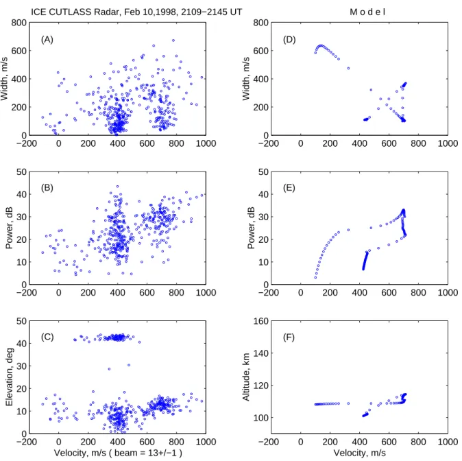
As a first step in exploring the data, we use an approach pro-posed by Milan and Lester (1999); namely, we make a scat-ter plot of the spectral width, power and elevation angle, as a function of the measured Doppler velocity. Such a presen-tation of radar data is known as a Watermann plot. In Fig. 4 we consider data from the Pykkvibaer beams 12, 13 and 14.
−2000 0 200 400 600 800 1000 10 20 30 40 50 Power, dB (B) −2000 0 200 400 600 800 1000 200 400 600 800 Width, m/s
ICE CUTLASS Radar, Feb 10,1998, 2109−2145 UT (A) −2000 0 200 400 600 800 1000 10 20 30 40 50 Elevation, deg Velocity, m/s ( beam = 13+/−1 ) (C) −2000 0 200 400 600 800 1000 10 20 30 40 50 Power, dB (E) −200 0 200 400 600 800 1000 100 120 140 160 Altitude, km Velocity, m/s (F) −2000 0 200 400 600 800 1000 200 400 600 800 Width, m/s M o d e l (D)
Fig. 4. Scatter plots illustrating width-velocity, power-velocity and elevation angle/altitude-velocity relationships, as observed (a-c) and as
predicted by the model (d-f).
In addition, we present matched model plots; details of the modeling will be described later.
Figure 4a shows that echoes are clustered in two distinctly different populations centred around 400 and 700 ms−1. No
clear trends can be seen within each cluster except for di-verging (spreading out) of their envelopes. The echo power, presented in Fig. 4b, also does not show any clear tendency, though one can recognise two peaks of power at 400 and 700 ms−1. Overall, the echo power is larger for the high-velocity cluster of points. The low-velocity points are more concen-trated around their central line near 400 ms−1 when com-pared to the spread of the high-velocity echoes about the 700 ms−1line. By comparing the scatter plots presented in Fig. 4a,b with the plots discussed by Milan and Lester (1999), one can identify the low-velocity echoes as class (i) echoes,
because velocities for these echoes are stable and close to the nominal ion-acoustic speed in the E-region. The high-velocity echoes can be identified either as class (iii) or class (iv) of Milan and Lester, as the average velocity is signifi-cantly more than 400 ms−1, and there is a fan-like data spread on the spectral width diagram.
Low elevation angles shown in Fig. 4c confirm that these echoes are, indeed, E-region echoes. An important feature of this diagram is that the high-velocity echoes (∼700 ms−1) have elevation angles that are larger by several degrees than the low-velocity (∼400 ms−1) echoes. One should note that for the low-velocity echoes, some points are located at very large elevation angles of about 45◦. We believe that these are “apparent” elevation angles; they occur due to the aliasing effect in the course of elevation angle measurements by the
6 8 10 12 14 600
650 700 750
Iceland CUTLASS Radar,Feb10,1998, 2112−2139 UT
Upper−Vel Plateau, m/s (A) 6 8 10 12 14 360 380 400 420 440 460 A n t e n n a B e a m N u m b e r (B) Lower−Vel Plateau, m/s
Fig. 5. Average echo velocity in various beams of the Pykkvibaer
HF radar on 10 February 1998, (a) for the high-velocity plateau data and (b) for the low-velocity plateau data. The dotted lines are cosine variations with the velocity maxima positioned at some beams.
phase interferometer. This typically happens when the mean elevation angle is less than the angle noise dispersion.
Figure 4d-f shows the echo parameters predicted by the model that will described in Sect. 5. We will discuss all the features of these panels later. At this point, we would like to mention that the majority of predicted points are grouped around velocities of 400 and 700 ms−1. A similarity between
the model-predicted echo populations and the observed ones is clear; the low-velocity echoes have a smaller power, lower heights (smaller elevation angles) and they are narrower than the high-velocity echoes. One should also realise that the model-predicted populations in panels (d-f), in reality, cor-respond to many closely spaced points, as one can infer by looking at the points in panel (e).
4 Flow angle variation for the mean velocity of the high-and low-velocity populations
In this section we study how the mean velocity of the high-and low-velocity populations changes with the azimuth (flow angle) of the measurements. Figure 5 shows the mean Dopp-ler velocity (the vertical bar through each point denotes the velocity error bar of the mean value) for a number of Pykk-vibaer beams, with distances of 495–675 km for the high-velocity echoes, and distances of 675–900 km for the low-velocity echoes. The dotted lines in Fig. 5 represent the co-sine flow angle variations (fitted to the experimental points) that one would expect if the velocity of ionospheric irregu-larities follow the linear theory formula. For the fitting, in accordance with the data trends, the maximum of the veloc-ity was assumed to be achieved at different beam numbers
for the high- and low-velocity echoes.
For the high-velocity echoes in Fig. 5a, one can see a clear velocity maximum in beam 13 and a velocity decrease with the beam number decrease. The velocity decrease cor-responds to an increase in the flow angle for the decreas-ing beam number (for the geometry, see Fig. 1). Such a flow angle variation of the velocity indicates that the high-velocity echoes are of class (iv), introduced by Milan and Lester (1999). For the low-velocity echoes in Fig. 5b, the velocity maximum was observed in beams 8–11, indicating a shift of about 15◦in the directions where the velocity max-ima were observed for the low- and high-velocity popula-tions. Also for the low-velocity echoes there is a gradual ve-locity decrease with beam number (from 11 to 15). This fea-ture does not fit class (i) echo characteristics, as described by Milan and Lester (1999); the flow angle variation for the low-velocity echoes is more reminiscent of the class (iii) echoes. Data presented in this and previous sections suggest that per-haps the classification scheme proposed by Milan and Lester (1999) is not complete; even more combinations of parame-ters are possible.
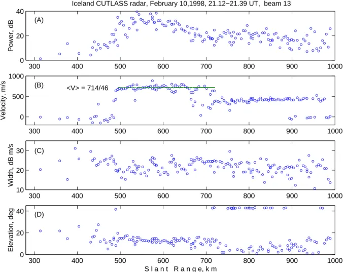
5 Slant-range profiles of echo parameters
Our next step is to present the echo parameters versus slant range. This approach was intensively utilised in paper 1. Fig-ure 6 presents echo parameters in beam 13 for the period of 2112–2139 UT. One should note that this diagram is not a direct plotting of experimental data; the actual resolution of measurements is 45 km while the points here are separated by only 5km. In constructing this diagram, we noticed that the echo band moved (as a whole) slowly equatorward dur-ing the interval of measurements. The mean speed of such echo region displacement was ∼2.2 km min−1so that the
to-tal shift of echoes was around 60 km (∼1 range gate). We selected a reference time of 2118 UT and a corresponding distance of the echo power maximum as base time and dis-tance. The positions of each point of slant range profiles at different times was then found using a linear range interpo-lation.
The power (Fig. 6a) exhibits a sharp increase at short dis-tances of 450–500 km and then reaches a plateau at disdis-tances ∼500–600 km, followed by a slow and smooth decrease at larger distances. The Doppler velocity diagram (Fig. 6b) shows two plateaus: the first one at ∼700 ms−1at distances of 500–700 km, and the second one at ∼400 ms−1at slant ranges of more than 700 km. At short distances (<500 km), the velocities are small and they reach a plateau in a very short band of ranges matched with the ranges of the sharp power increase. The velocity transition from the first plateau to the second one at ∼700 km is also very sharp. Similar power and velocity variations were observed in beams 11–14 (data not presented here).
The spectral width (Fig. 6c) does not show any clear ten-dencies. However, at the ranges where the velocity changes rapidly, there is an indication of an increase in the average
300 400 500 600 700 800 900 1000 0
20 40
Power, dB
Iceland CUTLASS radar, February 10,1998, 21.12−21.39 UT, beam 13 (A) 300 400 500 600 700 800 900 1000 0 500 1000 Velocity, m/s <V> = 714/46 (B) 300 400 500 600 700 800 900 1000 10 20 30 Width, dB m/s (C) 300 400 500 600 700 800 900 1000 0 20 40 Elevation, deg (D) S l a n t R a n g e, k m
Fig. 6. Experimental slant-range profiles for (a) echo power, (b) Doppler velocity, (c) spectral width, and (d) elevation angle.
spectral width. Note that the spectral width is presented in Fig. 6c in a logarithmic scale to better resolve changes of nearly two orders of magnitude in a span of the width.
In the transition area, the elevation angles (Fig. 6d) ex-hibit a sharp drop at ∼750 km, from the high- to low-velocity echoes, and the change in the elevation angle with distance is of the order of −0.4◦km−1. The regular elevation angle
change, which can be calculated for targets at the same height but at different slant ranges, is of the order of −0.02◦km−1. This indicates that the large-distance echoes come from lower heights. Modeling presented in Sect. 6 shows that the jump in the altitude of scatter at ∼750 km can simply be due to quick changes in scattering conditions at these ranges and not caused by an onset of a new irregularity layer at signifi-cantly smaller heights.
Slant range profiles of echo parameters clearly show that the two classes of echoes identified through the scatter plot analysis of Fig. 4 correspond to two distinctly different areas of the ionosphere. The high-velocity echoes (∼700 ms−1) are observed at shorter distances, from 500–700 km in beam 13–14, and approximately 500–600 km in beams 11–12 (the outer range edge gradually decreases toward smaller beam
numbers). The low-velocity echoes (∼400 ms−1) are ob-served at larger distances, between 700–1000 and 600–1000 km depending upon the beam number, respectively. None of the high-velocity echoes are seen in the second interval of distances and none of the low-velocity echoes are seen in the first interval of distances. There is a limited amount of very low velocity echoes, i.e. less than 100 ms−1, in both Fig. 4 and Fig. 6. The low velocity echoes which occur at short ranges may arise due to scatter from meteor trails. In this case, these velocities represent the neutral wind velocity between 80 and 100 km altitude. We omit these echoes from further consideration.
6 Modeling of slant-range profiles of echo parameters
Paper 1 explains many features in the slant range distribu-tions of the E-region HF echo parameters by employing a semi-empirical model of HF signal formation. Since range profiles, at least for the power, reported in this study are sim-ilar to those discussed in paper 1, it is logical to attempt a similar approach to the interpretation of other echo parame-ter variations. The main thrust of this section is to understand
400 500 600 700 100 110 120 0 5 −5 (A) Altitude, km 400 500 600 700 10 20 30 Power, dB (B) 400 500 600 700 200 400 600 800 (C) Velocity, m/s Slant Range, km 400 500 600 700 100 110 120 5 −5 0 (D) 400 500 600 700 10 20 30 (E) 400 500 600 700 200 400 600 800 (F) Slant Range, km
Fig. 7. (a) and (d): The model altitude-range distributions of the relative radar volume cross section represented by 20-dB step isolines and
by darkness of the tone for two N (h)-profiles (shown at the left-hand portions of the panels) with the electron density at a maximum of
0.65·1011m−3. The dots are the lines of zero and +/–5◦aspect angles. (b) and (e): The height-integrated power range profiles (solid lines).
The small dots on panel (e) illustrate the profile that would be observed in a case of a 45-km radar range resolution. (c) and (f): The predicted Doppler velocity (solid lines). The open-circles on panels (b-f) are the power-weighted height-integrated power and velocity of the in-cone
irregularity component (off-orthogonal angle magnitudes are less than 1.6◦), while crosses are the power and the velocity for the out-of-cone
irregularity component (off-orthogonal angle magnitudes are more than 1.6◦). The stars on panel (d) illustrate the range profile of the mean
backscatter altitude (for more details see text in Sect. 4). The vertical bars in the upper parts of panels (b), (c), (e), and (f) represent the range interval of the high-velocity echo observations (Fig. 6).
the reasons why two clusters of echoes were observed within one radar beam.
For the modeling, the following assumptions are made (similar to those in paper 1). It was assumed that the scat-ter comes only from E-region altitudes and that the resul-tant observed echo is a superposition of scattering at various heights. The signal contribution from each altitude was sumed to be determined by the electron density and the as-pect angle (which is dependent on the electron density). We postulated that the relative electron density fluctuation ampli-tude of ionospheric irregularities is altiampli-tude independent (to a first approximation), as experimentally found by Pfaff et al. (1984). The E-region was treated as a spherically symmetric one. To see the possible effects of the electron density distri-bution in the ionosphere, two electron density N (h) profiles
were selected, as depicted in the left portions of Fig. 7a,d. These electron density profiles have slightly different shapes but have the same maxima of 0.65·1011 m−3. To compute the amount of refraction, we used Snell’s law for the curved ionosphere so that the rectilinear radio wave propagation was assumed entirely until the point of scatter, where all of the re-fraction takes place. Such an approach treats rere-fraction prop-erly but slightly underestimates the slant ranges (and thus, overestimates the elevation angles). For computations of as-pect angles after refraction, the IGRF magnetic field model was used.
The choice of the maximum electron density significantly affects the predictions. Unfortunately, no direct density mea-surements were available within the Pykkvibaer field-of-view. As mentioned, we selected Ne = 0.65 · 1011 m−3.
This value is reasonable and further supported by the model-ing, which gives echo profiles that are, overall, very close to the observed ones. Additional support for our choice of the electron density comes from consideration of the slant range at which the echo power, the velocity and the width jump sharply (∼750 km). This slant range is very sensitive to the density value; it signifies the shortest range at which total reflection occurs close to the height of the electron density maximum. Computations for the selected electron density value are consistent with the observed ranges of echo param-eter jumps. Radar data suggest that for beams 11 and 12, the electron density should be slightly larger, (0.7–0.75)·1011 m−3.
The choice of the electric field intensity is also important for the modeling. In this respect, again, no supportive data were available. The observed E-region irregularity drift ve-locities of the order of 700 ms−1 suggest that the electric
field should be of the order of 60–70 mVm−1; this estimate
is based on VHF coherent radar Doppler velocity observa-tions and incoherent radar measurements of electric fields (Nielsen and Schlegel, 1983, 1985). An inspection of the Pykkvibaer channel 2 echoes does not show regular veloci-ties of larger than 700–1000 ms−1. However, we should note that the channel 2 F-region echoes (which we consider for the electric field estimates) were rather weak and probably contaminated by the low-velocity E-region echoes. Thus, it is very likely that the F-region velocities of 700–1000 ms−1, in reality, correspond to much stronger electric drifts.
The unfavourable conditions for the Pykkvibaer radar de-tection of clean F-region echoes is consistent with the Fin-land radar data; for this radar, there were no F-region echoes during the first half of the interval, and they were very weak for the second part of the period. We guess that the F-region electron density was slightly smaller than the one required for orthogonal F-region backscatter to occur. A similar con-clusion that the low F-region electron density was low (less than 1011 m−3) is drawn from the monthly median values of the critical frequencies for the Sodankyl¨a ionosonde, as reported by Milan et al. (1997). In spite of the generally unfavourable conditions for observations of F-region echoes, we found a short interval (several minutes), centred around 2124 UT, for which such echoes were observed by all three HF radars. Both Iceland radars registered velocities of 1300– 1500 ms−1. The physical cause for the simultaneous echo occurrence is probably a short-lived enhancement of soft au-roral precipitation. The Finland radar showed a power in-crease and a short equatorward inin-crease in the extent of the scattering region during this period; both features can be in-terpreted as signatures of enhanced precipitation.
Our choice of the electric field and of the electron den-sity value were also checked by considering the magnitude of the magnetic perturbations. By assuming that an infinite eastward current flow has a meridional width of the order of 100–200 km, we found that a disturbance of ∼40 nT would correspond to the current density of 0.22–0.13 Am−1. For the estimated height-integrated conductance of 4 S (by assuming the electron density profile with the peak value of 0.65·1011
m−3), such current densities would occur for electric fields of
55–35 mVm−1. Our E-field estimates can actually be even
higher since the Hall conductance can, in reality, be smaller; our radar model is not sensitive to the low-altitude end of the N (h)-profile so that smaller densities are acceptable. We should mention that since the magnetic field variations were slow, less than 1 nTmin−1, we could neglect the Earth induc-tion effects considered by Tanskanen et al. (2001).
For calculations of the Doppler velocity contribution from every altitude, we considered both in-cone and out-of-cone irregularities, similar to Kustov and Haldoupis (1992). We assumed that within the linear instability cone (in flow and aspect angles) there are type 1 irregularities, where the phase velocity was postulated to be the ion-acoustic speed modi-fied by turbulent heating, as discussed by Robinson (1986) and Robinson and Honary (1990). We used the average ion-acoustic speed height profile experimentally derived by Kustov et al. (1992). Since the largest electric field avail-able from the measurements of Kustov et al. (1992) was 65 mVm−1, we extrapolated those measurements to the elec-tric field of 70 mVm−1to have an order of magnitude fit of the predicted and observed velocities. The second velocity component from the out-of-cone irregularities was assumed to follow the simple linear fluid equation with altitude-dependent collision frequencies (Fejer and Kelley, 1980). A similar approach was adopted by Uspensky et al. (1994a). The E-region collision frequency profiles were based on EIS-CAT statistics, as described by Huuskonen (1989).
Model predictions of echo parameters for 2 electron den-sity profiles with maxima at 114 km altitude are presented in Fig. 7. Panels (a) and (d) illustrate the altitude-range profiles for the relative backscatter volume cross sections; this pa-rameter defines the spatial variations of all other quantities. The relative volume cross sections were corrected for the range attenuation, assuming the R−3dependence for a soft target. The solid lines are volume-cross section isolines with 20-dB steps; a darker shading helps in locating stronger local cross sections. The dotted lines show the spatial distributions of the true aspect angle (after refraction). The ±5◦isolines are well visible; the zero-aspect angle curve runs through the area of the largest volume cross sections. The stars in panel (d) represent the expected mean backscatter altitudes (see Eq. 5, paper 1). The predicted mean altitude corresponds to the elevation angle measured by an interferometer; both parame-ters are determined as power-weighted quantities in a certain gate (see paper 1).
The solid lines in Fig. 7b,e show the slant range profiles for the echo power and in Fig. 7c,f show the profiles for the Doppler velocity. Both parameters are height-integrated and power-weighted. For example, to calculate the Doppler velocity at a given range, all the contributions from each titude are first weighted according to the power at that al-titude (dependent upon the density), then summed, and fi-nally, normalised with respect to the number of points taken in the model profile and the total power. The full details of this calculation are given in paper 1. The only difference be-tween the pairs (b-c) and (e-f) is in the assumed shape of the
N (h)-profiles. One can see that the different density profiles give slightly different slant range distributions of echo pa-rameters; the most distinctly different are the “slopes” of the high-velocity plateaus, panels (c) and (f).
The open circles on power panels (b) and (e), which run along the solid power/velocity profiles (except at small ran-ges), and the crosses, which run below the profiles, indicate the relative contributions of the in-cone and out-of-cone ir-regularities to the height-integrated power, respectively. For large distances, the main contribution comes from the in-cone irregularities; the circles almost coincide with the line. For short ranges of less than 520–530 km, the only contribu-tion is from the out-of-cone irregularities. One should men-tion that the circles and crosses in panels (b) and (e) do not seem far apart, but the difference is significant; it is sim-ply hidden by the logarithmic presentation of the predicted power. For the velocity panels (c) and (f), the circles and crosses show what would be the velocity if only in-cone or out-of-cone irregularities were present.
We would like to mention several specific features seen in panels (b) and (e). First, the echo maxima occur at slant ranges of ∼580 km, where the aspect angle contour crosses the altitude of the electron density maximum. Second, there is a cutoff of the scatter from the top part of the irregularity layer at ranges larger than ∼690 km. This is a result of ra-dio wave reflection downwards at these ranges. Third, one can notice a very thin layer of moderate and weak backscat-ter from the bottom portion of the E-region for slant ranges larger than the cutoff range of 690–710 km. For these ranges, the altitude of backscatter is noticeably smaller; the drop in the mean altitude (stars in panel (d)) takes place at slant ranges larger than the cutoff range. One can see that the pre-dicted profiles of the echo power and the Doppler velocity of Fig. 7e,f agree reasonably well with the experimental data presented in Fig. 6a,b. For convenience, the two vertical lines at the top of panel (b), (c), (e) and (f) in Fig. 7 show the slant ranges of the high-velocity (∼700 ms−1) echoes. Note that the model predicts a quick drop in the backscatter eleva-tion angles at ranges around 700 km, which is in agreement with the experimental data (see Fig. 6d). There are some mi-nor differences between the model and the experiment. For example, Fig. 7f shows that the leading edge of the model velocity profile is shifted ∼25 km farther than the observed profile. We will discuss this point in more detail later. And finally, we show in panel (e) (dotted line) the power profile performed with a 45-km range resolution just to illustrate that limited radar resolution would not seriously affect the model predictions. The dotted profile is the 45-km running mean of the basic power profile of Fig. 7e. In a similar way, we build the range-power profile from experimental data. We overlap adjacent dwell-cycle echoes from a common echo band, as it moves slowly equatorward.
After demonstrating a reasonable agreement between mo-del predictions and observed slant range distributions of echo parameters, we compare predictions with experimental data presented in Fig. 4 in the form of scatter plots. To accom-plish this, we plotted in Fig. 4d-f the model parameter
val-ues versus velocity (instead of elevation angles, we presented the expected height of scatter). To find the expected spectral width, we assumed (in accordance with paper 1) that the in-herent spectral width of irregularities is altitude-independent and amounts to 100 ms−1. We calculate the model spectral widths by the integration of scattering irregularities at differ-ent heights and, therefore, differdiffer-ent velocities. Data cluster-ing near velocities of 400 ms−1and 700 ms−1is seen in panel (e), although there are additional weaker echoes for small ve-locities of 200 ms−1. The latter small-velocity echoes are short distance echoes due to the out-of-cone irregularities; they were not observed experimentally, perhaps due to a poor radar sensitivity. As we briefly commented in Sect. 3, the ex-perimental Watermann plots and the model distributions are in reasonable agreement.
7 Discussion
In this study, we demonstrated several important features of the high-velocity E-region HF echoes. We showed that such echoes can be seen in several radar beams for observations roughly along magnetic L-shells. When the echo power and the spectral width were sorted according to their Doppler ve-locity, it turned out that even for a short time interval of ∼30 minutes, the echoes can cluster into two distinctly differ-ent populations on the plots: the low-velocity (∼400 ms−1) and high-velocity (∼700 ms−1) populations. One might con-clude, following Milan and Lester (1999), that two classes of echoes/ionospheric irregularities coexisted during the event considered. When the data were plotted versus slant range, we demonstrated that different populations of echoes corre-sponded to different slant ranges, i.e. to different areas of the high-latitude ionosphere. This might still be considered as an indication of two physically different areas of the ionosphere with different magnitudes of the ambient electric field. One might even think about two different instabilities operational in these distinctly different areas.
Villain et al. (1987, 1990) considered HF E-region obser-vations under comparable conditions. Their slant range pro-files for the power and velocity had many features similar to those reported in this study and in paper 1. They also found two types of echoes, one with relatively large Doppler veloc-ities (∼580 ms−1), and another one with smaller velocities (∼445 ms−1). In addition, jumps in the velocity and spectral width at some ranges were reported. The ratio of the high-to low-velocity was determined high-to be about 1.35 (Villain et al., 1987) and more than 2 (Villain et al., 1990). These ratios are both close to the values we can calculate here of ∼1.7. Villain et al. (1990) concluded that the echoes with moder-ate velocities were associmoder-ated with the secondary gradient-drift instability, while the higher-velocity echoes with ve-locities of 400–550 ms−1were attributed to the ion-acoustic waves driven by a combination of the parallel and perpendic-ular electron drifts at altitudes of ∼120 km. Thus, Villain et al. (1990) suggested that the low- and high-velocity echoes originate from two different irregularity layers, separated in
height (though both within the E-region).
To explain HF slant range profiles, reported both previ-ously and in this study, we used a model of HF signal forma-tion, proposed originally by Uspensky (1985) and expanded later by Uspensky and Williams (1988) and Uspensky et al. (1989). This model assumes that echoes are received from a range of electrojet heights and that the power of the signal from each height is determined by the local electron density, the true aspect angle (with the refraction taken into account), and the amplitude of the ionospheric irregularities (Oksman et al., 1986; Kustov et al., 1990; Williams et al., 1999). For strong electric fields of more than 30–40 mVm−1, it is as-sumed that the irregularity amplitude is electric-field-inde-pendent, so that irregularity amplitude flow and aspect angle variations need only to be taken into account. The variation of the irregularity amplitude with the electric field can be incorporated into modeling if an exact form of the relation-ship is known, which is definitely important for small electric fields.
Our modeling shows that one might have two distinct ters of echoes in the Watermann plots and each of these clus-ters would correspond to type 1 waves, but observed at dif-ferent altitudes due to difdif-ferent amounts of HF radio wave re-fraction at various slant ranges. For example, at far distances, echoes can only come from the bottom part of the E-region. Thus, we interpret two clusters of echoes as a consequence of a radio wave focusing to different parts of the E-region, and not due to distinctly different irregularity layers. Different irregularity phase velocities occur for different altitudes be-cause of the variation of the ion-acoustic speed with altitude, e.g. Kustov et al. (1992) and Nielsen and Schlegel (1983). Thus, physically our interpretation is close to, but not similar to the Villain et al. (1990) interpretation.
The main points of our understanding of the E-region HF auroral backscatter for L-shell directions are the following:
1. Main power-contributing echoes are scatter from in-cone, type 1 irregularities.
2. At moderate distances, scatter from these irregularities is important in the central part of the E-region. Depend-ing on the electron density profile, contributions can come from altitudes slightly above or below the density maximum.
3. At farther distances, where radio wave reflection occurs at altitudes near the electron density maximum, the au-roral backscatter comes from altitudes below the elec-tron density maximum (bottom of the E-region). 4. Secondary out-of-cone irregularities exist in a much
wi-der range of directions than the primary irregularities (including the linear instability cone). However, these irregularities are visible only to radars at short distances, since here the near-perfect orthogonality of radar waves with the magnetic field lines cannot be achieved. Thus, the primary waves are blocked from detection. In this respect, short distances are unique; only here can one see directly the aspect angle effects in echo parameters.
St.-Maurice et al. (1994) proposed an alternative interpre-tation of the high velocity echoes. These authors argued that large velocity waves are simply the F-B waves excited in the presence of strong plasma gradients and electric fields. Ac-cording to this interpretation, the present observations and the observations by Villain et al. (1987, 1990) can be consis-tently explained. To apply the interpretation by St-Maurice et al. (1994) to the observations, however, one has to be sure that strong plasma gradients associated, for example, with auroral arcs, were present. We do not have data to support or reject this interpretation.
A good fit of the model and experimental data gives us ad-ditional confidence that the Uspensky et al. (1994a) approach properly describes the way the auroral E-region echoes are formed at HF. One important conclusion of the model is that even for a spatially uniform ionosphere, HF E-region echo occurrence should be limited to certain distances of 150– 250 km in their extent, even though ionospheric irregulari-ties may exist over a much larger area. An HF radar simply cannot detect irregularities outside the area of exact orthog-onality or acceptable non-orthogorthog-onality. If one applies the model to various azimuths, a tendency for the L-shell align-ment of both channel 1 and channel 2 echoes (Milan and Lester, 1998) can be demonstrated. Indeed, for observations perpendicular to the L-shells, the distances of near zero as-pect angles are smaller and thus, the echo power should have a maximum at shorter distances. This tendency has been pre-dicted by Uspensky et al. (1989) for the VHF band.
In this study, similarly to paper 1, we show that iono-spheric refraction is an extremely important factor to be con-sidered at HF. This fact is indisputable (Unwin, 1966; Green-wald et al., 1985; Moorcroft, 1989; Uspensky, 1985; Us-pensky et al., 1994a,b). However, only a few papers, in the past, have emphasised the fact that even in the simplest case, in which irregularities exist at all heights, refraction makes certain heights more efficient in terms of scatter so that the range-altitude distribution of the volume cross section has a crescent-like configuration, as shown in Fig. 7a,d. One should note that a similar cross section configuration is ex-pected for F-region backscatter. It is important to realise that a crescent-like configuration for the cross section is a com-mon topological image of the backscatter configuration in an anisotropic medium. It means that other E-region echo pa-rameters, such as the Doppler velocity and the spectral width, are strongly refraction-dependent. Thus, our modeling sug-gests that in order to infer properties of E-region irregularities from HF radar data, all refraction-related effects (as precisely as possible) should first be taken into account. Clearly, for a patchy ionosphere, this is a very complicated task.
Our observations showed that the high-velocity and low-velocity echoes obtain maxima at different azimuths (Fig. 5); the low-velocity echoes have their maximum in beams 8–11, while the high-velocity echoes have their maximum in beam 13. We also found experimentally and predicted through modeling that these two types of echoes have differ-ent altitudes. It is well known that the F-B instability has a larger growth rate in the direction of the relative drift between
the electrons and ions. Since this drift direction changes with height, one would expect that the high-velocity echoes (larger heights) would be observed at slightly different az-imuths than the low-velocity echoes (lower heights). If the electron drift was L-shell-aligned at the bottom of the elec-trojet layer (and it was roughly matched to the low-velocity echo maximum), then, due to current rotation with the height, one would expect that the high-velocity echoes would have the largest velocities at azimuths, counter clockwise from the L-shell direction when looking along the magnetic field line from above, i.e. for smaller beam numbers, as compared to the low-velocity echoes. Our measurements do not support this notion; we observed just the opposite difference in the azimuth (beams 8–11 for the low-velocity echoes and beam 13 for the high-velocity ones). The issue, however, requires further studies. We would like to note that if one assumes that the velocity of decametre irregularities follows the linear theory formula, then one would expect the maximum irregu-larity velocities to be observed not along the direction of the electron-ion relative drift, but along the sum of electron and ion velocity modified by collision frequencies, i.e. 10–15◦ away from the E×B direction. For the electric field direction assumed in this study (northward), the velocity maximum at larger heights should then be in beam 13, as observed. Ex-perimentally, Mattin and Jones (1987) reported on the flow angle asymmetry of VHF scatter and it cannot simply be ex-plained by the rotation of the current with the height, as in our measurements at HF. On the other hand, Abel and Newell (1969) observing with the UHF Millstone Hill radar perpen-dicular to the L-shells, found that the azimuth of the Doppler velocity reversal changed in accordance with the electrojet rotation with height.
In the course of our modeling, several assumptions were made regarding the electron density profiles and the electric field in the ionosphere. This allowed us to find a reason-able agreement between the model and observations. We un-derstand that independent incoherent scatter radar measure-ments of the ionospheric parameters are required to make the modeling more reliable and this is in our plans. Here, we would like to make several comments on some disagreements between the predictions and observations.
First of all, we would like to mention that we presented experimental data (Fig. 6) for beam 13, while we performed modeling (Fig. 7) for beam 12. In doing so, we kept in mind that data in beam 13 were collected from a range of direc-tions, including the beam 12 azimuth (two-way 3-dB antenna beamwidth is ∼5◦broad and the separation between
neigh-bouring beam positions is ∼3.3◦).
Now, let us concentrate on the slant range positions of the sharp echo power and velocity jumps at short and large dis-tances. To a first approximation, model predictions, for ex-ample, shown in Fig. 7d-f, match the experimental profiles well. However, as we mentioned, a closer look reveals that the sharp increase of the velocity at short distances is located about 25 km farther away than the experimentally observed distances of the velocity jump (see vertical bars at the top of each panel). Any attempt to shift the area of the
veloc-ity increase to closer distances, either by increasing electron density or decreasing the E-region height, creates a two times larger shift of the region, where the power and velocity jump down at distances of ∼750 km. We found that this discrep-ancy can be understood if one takes into account the fact that the Pykkvibaer radar worked, in reality, in a frequency band of 10.2–10.6 MHz (not at the mean frequency of 10.35 MHz, used in our modeling). Modeling using various frequencies shows that the echo region of the sharp velocity increase can be shifted by 15–20 km to closer ranges at smaller radar fre-quencies within the above band. The location of the far-range sharp velocity decrease is also frequency-dependent. According to modeling for various radar frequencies, there should be a band of ranges ∼50 km, where the velocity de-creases near 750 km. This prediction agrees with measure-ments shown in Fig. 6b, where a cloud of points is spread between 670 and 720 km. We can conclude that knowledge of the ionospheric parameters, as well as all the details of the measurements is important for achieving a better agreement between the model predictions and observations.
8 Summary
In this study, we presented data from the Pykkvibaer HF radar of high-velocity E-region echoes on 10 February 1998. Similar high-velocity echoes were detected by the Stokkseyri HF radar that monitored about the same range of magnetic latitudes, but to the west from the Pykkvibaer field-of-view. We showed that the Pykkvibaer echoes on the power-velocity scatter diagram were clustered around two values of veloc-ity: 700 ms−1and 400 ms−1. Echoes of the first cluster were
generally stronger than the second one. The spectral width-velocity scatter plots exhibited a fan-like configuration for both clusters of echoes. By studying the range profiles of the echoes, we discovered that the high-velocity (∼700 ms−1) echoes were coming from shorter distances and higher ele-vation angles than the low-velocity echoes. Echo parameters plotted versus slant range displayed synchronised variations. At the shortest distances, both the power and the Doppler velocity showed an increase. After reaching maxima, they both stabilised their increase and were more or less constant for about 200 km. At larger distances, they sharply dropped down; power decreased by 10–20 dB and the velocity de-creased by a factor of ∼0.59. At ranges near these drops, the echo spectral width seems to be increased.
In an attempt to explain the relationship and variations of echo parameters, we assumed that the ionosphere was uni-form in latitude and longitude and that a constant electric field of the order of 70 mVm−1was set up within the radar field-of-view. We then applied the model of auroral echo for-mation considered by Uspensky et al. (1994a), to predict the distribution of echo parameters with distance. While mod-eling, it was assumed that the conventional type 1 and type 2 irregularities were present within the radar field-of-view. Contributions of each type of echoes to the resultant signal were computed on the basis of their properties and the real
aspect angle conditions controlled by ionospheric refraction. A good agreement between predictions and measurements was found, giving a chance to say that the discovered two clusters of points are a result of radar wave focusing to the central and bottom of the electrojet layer at short and far dis-tances, respectively. The high and low velocity echoes were both due to type 1 waves. We conclude that the ionospheric refraction is so significant at HF that to infer properties of decametre-scale irregularities from regular observations, the propagation effects have to be taken into account as much as possible. One of the ways to do such work is to consider coordinated HF radar observations with incoherent scatter radars.
Acknowledgements. This work was supported by the Academy of
Finland, and, additionally, by the Canadian NSERC grant to AVK and by the Swedish Royal Academy of Sciences grant to MVU. The authors thank Drs A. Viljanen (FMI), J. Waterman, V. Petrov (DMI) and T. Saemundsson (University of Iceland) for IMAGE, Greenland, and Iceland magnetometer data and related computa-tions. Comments from both referees were greatly appreciated.
The Editor in Chief thanks P. Erikson and another referee for their help in evaluating this paper.
References
Abel, W. G. and Newell, R. E., Measurements of the afternoon radio aurora at 1295 MHz, J. Geophys. Res., 74, 231–245, 1969. Eglitis, P., Robinson, T. R., McCrea, I. W., Schlegel, K., Nygren, T.,
and Roger, A. S., Doppler spectrum statistics obtained from three different-frequency radar auroral experiment, Ann. Geophysicae, 13, 56–65, 1995.
Fejer, B. G. and Kelley, M. C., Ionospheric irregularities, Rev. Geo-phys., 18, 401–454, 1980.
Greenwald, R. A., Baker, K. B., Hutchins, R., and Hanuise, C., An HF phased-array for studying small-scale structure in high-latitude ionosphere, Radio Sci., 20, 63–79, 1985.
Greenwald, R. A., Baker, K. B., Dudeney, J. R., Pinnock, M., Jones, T. B., Thomas, E. C., Villain. J.-P., Cerisier, J.-C., Senior, C., Hanuise, C., Hunsucker, R. D., Sofko, G., Koehler, J., Nielsen, E., Pellinen, R., Walker, A. D. M., Sato, N., and Yamagishi, H., DARN/SUPERDARN, Space Sci. Rev., 71, 761–796, 1995. Haldoupis, C., A review on radio studies of auroral E-region
iono-spheric irregularities, Ann. Geophysicae, 7, 239–258, 1989. Hamza, A. and St-Maurice, J.-P., A self-consistent fully turbulent
theory of auroral E-region irregularities, J. Geophys. Res., 98, 11601–11613, 1993.
Hanuise, C., Villain, J.-P., Cerisier, J. C., Senior, C., Ruohoniemi, J. M., Greenwald, R. A., and Baker, K. B., Statistical study of high-latitude E-region Doppler spectra obtained with SHERPA HF radar, Ann. Geophysicae, 9, 273–285, 1991.
Huuskonen, A., High resolution observations of the collision fre-quency and temperatures with the EISCAT radar, Planet. Space Sci., 37, 211–221, 1989.
Jayachandran, P. T., St-Maurice, J.-P., MacDougall, J. W., and Moorcroft, D. R., HF detection of slow long-lived E-region plasma structures, J. Geophys. Res. 105, 2425–2442, 2000. Jones, B., Williams, P. J. S., Schlegel, K., Robinson, T., and
Hag-gstrom, I., Interpretation of enhanced electron temperatures
mea-sured in the auroral E-region during the ERRRIS campaign, Ann. Geophysicae, 9, 55–59, 1991.
Kustov, A. V., Uspensky, M. V., Kangas, J., Huuskonen, A., and Nielsen, E., Effect of altitude profile of auroral scattering on electric field measurements in the STARE experiment, Geomagn. Aeron., 30, 384–388, 1990.
Kustov, A. V. and Haldoupis, C., Irregularity drift velocity estimates in radar auroral backscatter, J. Atmos. Terr. Phys., 54, 415–423, 1992.
Kustov, A. V., Virdi, T., Williams, P. J. S., and Jones, G. O. L., The ion-sound velocity in the auroral E-region from EISCAT measurements in August 1988, Geomagn. Aeron., 32, 248–251, 1992.
Koustov, A. V., Igarashi, K., Ohtaka, M., Sato, N., Yamagishi, H., and Yukimatu, S., Nearly simultaneous observations of VHF and HF E-region coherent echoes at the Antarctic Syowa station, J. Geophys. Res., 106, 2001 (in press).
Mattin, N. and Jones, T. B., Propagation angle dependence of radar auroral E-region irregularities, J. Atmos. Terr. Phys., 49, 115– 121, 1987.
Milan, S. E., Yeoman, T. K., Lester, M., Thomas, E. C., and Jones, T. B., Initial backscatter occurrence statistics from the CUT-LASS HF radars, Ann. Geophysicae, 15, 703–718, 1997. Milan, S. E. and Lester, M., Simultaneous observations at
differ-ent altitudes of ionospheric backscatter in the eastward electrojet, Ann. Geophysicae, 16, 55–68, 1998.
Milan, S. E. and Lester, M., Spectral and flow-angle characteristics of backscatter from decametre irregularities in the auroral elec-trojets, Adv. Space Res., 23, 1773–1776, 1999.
Moorcroft, D. R., An explanation for VHF auroral backscatter at large aspect angles, Geophys. Res. Lett., 16, 235–238, 1989. Nielsen, E. and Schlegel, K., A first comparison of STARE and
EIS-CAT drift velocity measurements, J. Geophys. Res., 88, 5745– 5750, 1983.
Nielsen, E. and Schlegel, K., Coherent radar Doppler measurements and their relationship to the ionospheric electron drift velocity, J. Geophys. Res., 90, 3498–3504, 1985.
Nielsen E., Aspect angle dependence of mean Doppler velocities of 1-m auroral plasma waves, J. Geophys. Res., 91, 10173–10177, 1986.
Ogawa, T., Balsley, B. B., Ecklund, W. L., Carter, D. A., and John-ston, P. E., Aspect angle dependence of irregularity phase veloc-ity in the auroral electrojet, Geophys. Res. Lett., 7, 1081–1084, 1980.
Oksman, J., Uspensky, M. V., Starkov, G. V., Stepanov, G. S., and Vallinkoski, M., The mean fractional electron density fluctuation amplitude derived from auroral backscatter data, J. Atmos. Terr. Phys., 48, 107–113, 1986.
Pfaff, R. F., Kelley, M. C., Fejer, B. G., Kudeki, E., Carlson, C. W., Pedersen, A., and Hausler, B., Electric field and plasma density measurements in auroral electrojet, J. Geophys. Res., 89, 236– 244, 1984.
Robinson, T. R., Towards a self-consistent non-liner theory of radar auroral backscatter, J. Atmos. Terr. Phys., 48, 417–422, 1986. Robinson, T. R. and Honary, F., A resonance broadening kinetic
the-ory of the modified two-stream instability: implication for radar auroral backscatter experiments, J. Geophys. Res., 95, 1073– 1085, 1990.
Sahr, J. D. and Fejer, B. G., Auroral electrojet plasma irregularity theory and experiment: A critical review of present understand-ing and future directions, J. Geophys. Res., 101, 26893–26909, 1996.
Schlegel, K., Coherent backscatter from ionospheric E-region plasma irregularities, J. Atmos. Terr. Phys., 58, 933–941, 1996. St-Maurice, J.-P., Prykril, P., Danskin, D. W., Hamza, A. M., Sofko,
G. J., Koehler, J. A., Kustov, A., and Chen, J., On the origin of narrow non-ion-acoustic coherent radar spectra in the high lati-tude E-region, J. Geophys. Res., 99, 6447–6474, 1994.
Tanskanen, E. I., Viljanen, A., Pulkkinen, T. I., Pirjola, R., Hakki-nen, L., PulkkiHakki-nen, A., and Amm, O., At substorm onset, 40% of AL comes from underground, J. Geophys. Res., 2001 (in press). Unwin, R. S., The importance of refraction in troposphere and iono-sphere in determining the aspect sensitivity and height of radio aurora, J. Geophys. Res., 71, 3677–3686, 1966.
Uspensky, M. V., On the altitudinal profile of auroral radar backscatter, Radio Sci., 20, 735–739, 1985.
Uspensky, M. V. and Williams, P. J. S., The amplitude of auroral backscatter: 1. Model estimates of the dependence on electron density, J. Atmos. Terr. Phys., 50, 73–79, 1988.
Uspensky, M. V., Starkov, G. V., Stepanov, G. S., and Williams, P. J. S., The amplitude of auroral backscatter: 2. Topology of the backscatter range-azimuth distribution, J. Atmos. Terr. Phys., 51, 929–936, 1989.
Uspensky, M. V., Kustov, A. V., Sofko, G. J., Koehler, J. A., Villain, J.-P., Hanuise, C., Ruohoniemi, J. M., and Williams, P. J. S.,
Ionospheric refraction effects in slant range profiles of auroral HF coherent echoes, Radio Sci., 29, 503–517, 1994a.
Uspensky, M. V., Williams, P. J. S., Romanov, V. I., Pivovarov, V. G., Sofko, G. J., and Koehler, J. A., Auroral radar backscatter at off-perpendicular aspect angles due to enhanced ionospheric refraction, J. Geophys. Res., 99, 17503–17509, 1994b.
Uspensky, M. V., Eglitis, P., Opgenoorth, H., Starkov, G., Pulkki-nen, T., and PelliPulkki-nen, R., On auroral dynamics observed by HF radar: 1. Equatorward edge of the afternoon-evening diffuse lu-minosity belt, Ann. Geophysicae, 18, 1560–1575, 2001. Villain, J.-P., Greenwald, R. A., Baker, K. B., and Ruohoniemi,
J. M., HF radar observations of E-region plasma irregularities produced by oblique electron streaming, J. Geophys. Res., 92, 12327–12342, 1987.
Villain, J.-P., Hanuise, C., Greenwald, R. A., Baker, K. B., and Ruohoniemi, J. M., Obliquely propagating ion-acoustic waves in the auroral E-region: Further evidence of irregularity produc-tion by field-aligned electron streaming, J. Geophys. Res., 95, 7833–7846, 1990.
Williams, P. J. S., Jones, B., Kustov, A. V., and Uspensky, M. V., The relationship between E-region electron density and the power of auroral coherent echoes at 45 MHz, Radio Sci., 34, 449–457, 1999.