Anthropogenic carbon in the eastern South Pacific Ocean

(1)

HAL Id: hal-00330244

https://hal.archives-ouvertes.fr/hal-00330244

Submitted on 19 Jun 2007

HAL is a multi-disciplinary open access

archive for the deposit and dissemination of sci-entific research documents, whether they are pub-lished or not. The documents may come from teaching and research institutions in France or abroad, or from public or private research centers.

L’archive ouverte pluridisciplinaire HAL, est destinée au dépôt et à la diffusion de documents scientifiques de niveau recherche, publiés ou non, émanant des établissements d’enseignement et de recherche français ou étrangers, des laboratoires publics ou privés.

Anthropogenic carbon in the eastern South Pacific

Ocean

L. Azouzi, R. Gonçalves Ito, Franck Touratier, Catherine Goyet

To cite this version:

L. Azouzi, R. Gonçalves Ito, Franck Touratier, Catherine Goyet. Anthropogenic carbon in the eastern South Pacific Ocean. Biogeosciences Discussions, European Geosciences Union, 2007, 4 (3), pp.1815-1837. �hal-00330244�

(2)

BGD

4, 1815–1837, 2007

Anthropogenic carbon in the Pacific

Ocean L. Azouzi et al. Title Page Abstract Introduction Conclusions References Tables Figures ◭ ◮ ◭ ◮ Back Close Full Screen / Esc

Printer-friendly Version Interactive Discussion

EGU

Biogeosciences Discuss., 4, 1815–1837, 2007 www.biogeosciences-discuss.net/4/1815/2007/ © Author(s) 2007. This work is licensed

under a Creative Commons License.

Biogeosciences Discussions

Biogeosciences Discussions is the access reviewed discussion forum of Biogeosciences

Anthropogenic carbon in the eastern

South Pacific Ocean

L. Azouzi1, R. Gonc¸alves Ito2, F. Touratier1, and C. Goyet1 1

BDSI, Universit ´e de Perpignan, 52 avenue Paul Alduy, 66860 Perpignan, France 2

Instituto Oceanogr áfico, Universidade de S ão Paulo, Pça. do Oceanogr áfico, 191 Cidade Universit ária, 05508-900 S ão Paulo-SP, Brasil

Received: 23 February 2007 – Accepted: 27 February 2007 – Published: 19 June 2007 Correspondence to: L. Azouzi (azouzi@univ-perp.fr)

(3)

BGD

4, 1815–1837, 2007

Abstract

We present results from the BIOSOPE cruise in the eastern South Pacific Ocean. In particular, we present estimates of the anthropogenic carbon C_antTrOCAdistribution in this area using the TrOCA method recently developed by Touratier and Goyet (2004a, b) and Touratier et al. (2007). We study the distribution of this anthropogenic carbon tak-5

ing into account of the hydrodynamic characteristics of this region. We then compare these results with earlier estimates in nearby areas of the anthropogenic carbon as well as other anthropogenic tracer (CFC-11). The highest concentrations of C_antTrOCA are located around 13◦S 132◦W and 32◦S 91◦W, and their concentrations are larger than 80 µmol kg−1and 70 µmol kg−1, respectively. The lowest concentrations were ob-10

served below 800 m depths (≤2 µ mol kg−1) and at the Oxygen Minimum Zones (OMZ), mainly around 140◦W (<11 µmol kg−1). The comparison with earlier work in nearby areas provides a general trend and indicates that the results presented here are in general agreement with previous knowledge. This work further improves our under-standing on the penetration of anthropogenic carbon in the eastern Pacific Ocean. 15

1 Introduction

Studies on the fate of anthropogenic CO2 in the ocean interior are essential for

under-standing the global carbon cycle and its consequences on climate change and/or on the ocean itself (mainly due to its pH change induced by CO₂acidification) (Doney and Ducklow, 2006).

20

In order to understand the role of the oceans as a sink for anthropogenic CO2, it

is important to determine the distribution of carbon species in the ocean interior as well as the processes affecting the transport and storage of CO2 taken up from the

atmosphere (Chen and Millero, 1979; Peng et al., 2003).

Estimates of anthropogenic CO₂concentrations in the oceans have been improved 25

(4)

BGD

4, 1815–1837, 2007

EGU

based upon various model assumptions that often cannot be verified.

Following the main trends the anthropogenic CO₂is not evenly distributed throughout the oceans (Chen, 1982; Wong and Matear, 1993). While the ocean is known to be globally a sink for anthropogenic CO2(Chen and Millero, 1979; Brewer Peter G., 1997),

little anthropogenic carbon is stored in some specific regions such as the equatorial 5

belt.

Yet the equatorial belt (from 10◦N to 10◦S) plays a significant role in the global carbon cycle (Le Borgne et al., 2002). It annually supplies approximately 0.7–1.5 Pg C as CO2 gas to the atmosphere, and it is the largest natural source of CO2 from the

ocean (Takahashi et al., 1997; Feely et al., 1999). In particular, as much as 72% of the 10

CO₂outgassing from the world’s oceans can be attributed to the equatorial Pacific. The South Pacific Ocean (from the equator down to 60◦S) is globally considered as a sink area for anthropogenic carbon (Chen and Chen, 1993), but there is a strong zonal variability. Indeed, the western equatorial zone is the largest oceanic source of CO2 to the atmosphere, while the eastern equatorial (Tans et al., 1990; Murray et

15

al., 1992; Murray et al., 1995) is considered as CO2 sink. Here we present results

from the BIOSOPE (BIogeochemistry & Optics SOuth Pacific Experiment) cruise in the eastern (East of 142◦W) South Pacific Ocean along a ∼8000 km transect a gradient (Fig. 1). This transect covered a variety of hydrodynamic and trophic properties from the extremely rich upwelling waters of the Chilean coasts to the extremely oligotrophic 20

waters of the central gyre of the South Pacific Ocean, a priori expected to be the poorest oceanic area of the world (Longhurst, 1998; Claustre et al., 2007).

These specific zones could play a major role on CO₂ sequestration by the way of biological activity, thus taking up a significant amount of anthropogenic carbon from the atmosphere (Archer et al., 1996; Sabine and Key, 1998). Here, we use the data 25

from the BIOSOPE cruise to estimate the anthropogenic carbon. The TrOCA method recently developed by Touratier and Goyet (2004a, b), and Touratier et al. (2007) is then applied. We study the distribution of this anthropogenic carbon taking into account the hydrodynamic characteristics of the area. We then compare these results with those

(5)

BGD

4, 1815–1837, 2007

Printer-friendly Version Interactive Discussion of tracer (CFC-11) distributions and with earlier estimates of the anthropogenic carbon

in nearby areas.

2 Material and methods

2.1 Sampling

The BIOSOPE cruise onboard R/V ATALANTE, was conducted during austral summer 5

(26 October–12 December). The eastern South Pacific part was studied, especially the oligotrophic area associated to the central part of the South Pacific Gyre (SPG) along a latitudinal transect starting from the Marquises Islands around 70◦W 8◦S to the Peru coast at 141◦W 35◦S (Fig. 1).

Water sampling and measurements of temperature and salinity were made using 10

a SeaBird SBE 911plus CTD/Carousel system fitted with an SBE 43 oxygen sensor. From the 223 vertical profiles, 23 were sampled for studying the oceanic carbon cycle (Fig. 1). At each of these stations an average of 22 samples was collected throughout the water column from the near surface (∼3 m depth) to 500 m (excepted for 3 stations to the near bottom depth (>2000 m)).

15

Seawater was sampled into 500 ml borosilicate bottles and then after poisoned with a saturated solution of mercuric chloride before being sealed. They were then stored and shipped back to the laboratory where the measurements have been performed within one month after the end of the cruise

2.2 Parameter measurements 20

Total dissolved inorganic carbon (CT) and Total Alkalinity (AT) were determined by

the potentiometric acid titration method (DOE, 1994). From replicate analysis of a reference seawater sample of known AT concentration, (CRM from Dr Andrew

(6)

BGD

4, 1815–1837, 2007

EGU

analyses were determined to be within 1.5 µmol kg−1 for CT and 1.7 µmol kg

−1

for AT. In this study, we use also salinity (S), potential temperature (θ;

◦

C), oxygen (O2;

µmol kg−1), potential density (σ_θ; kg m−3), parameters measured on board. Oxygen (O2; µmol kg

−1

) was measured using a photometric endpoint detector and a piston burette (Metrohm, Dosimat 716); dissolved oxygen was determined using a protocol 5

taken from “WHP Operations and methods” (Culberson, 1991).

Next we calculate the anthropogenic CO₂concentrations (CTrOCA_ant ) using the TrOCA (Tracer combining Oxygen, inorganic Carbon and total Alkalinity) approach devel-oped by Touratier and Goyet (2004a, b) and Touratier et al. (2007). We then com-pare these results with the anthropogenic CO2concentrations (C∆C∗ant ) estimated earlier

10

(http://cdiac.ornl.gov/ftp/oceans/Pacific GLODAP ODV) using the ∆C* method (Gruber et al., 1996) and the WOCE and the JGOFS data sets.

3 Results and discussion

3.1 Hydrography and circulation

This research concerns seawater dominated by both the South Equatorial Current and 15

the Peru Current. The region can be roughly separated in five main areas (Claustre et al., 2007): (1) the Sub Equatorial area (142◦W–132◦W) (near the Marquise Islands) that is influenced by the equatorial regime; (2) the transition zone (132◦W–123◦W) between the sub Equatorial area and the South Pacific Gyre (SPG); (3) the central part of the SPG (123◦W–101◦W); (4) the transition zone between the SPG and the coastal 20

upwelling area (100 W◦–81◦W); (5) the coastal upwelling area (East of 81◦W).

The hydrography of the region is summarized by the θ-S diagram shown in the Fig. 2. Both the easterly winds which drive away the superficial waters and the prevailing southerly winds off the Peruvian coast provoke an upwelling along the equator and the Peruvian coast. The cold and relatively low-salinity waters of the Humboldt Current are 25

(7)

BGD

4, 1815–1837, 2007

Printer-friendly Version Interactive Discussion advected northward from Chile to offshore of Peru (Strub et al., 1998; Kessler, 2006).

These eastern boundary waters merge to supply the westward-flowing South Equato-rial Current (SEC), which is subject to the divergence, north and south of the equator, and generates upwelling of waters which brings waters with higher salinity, C_T, and nu-trient concentrations to the surface (Kessler, 2006). Since chlorophyll concentrations 5

remain low and the macronutrients are not depleted, this region is called the HNLC (high-nutrient/low-chlorophyll) area (Minas et al., 1986).

In the SEC (South Equatorial Current) the surface seawater is characterized by the warm and high-salinity SubTropical Surface Water (STSW, S>35). Along the coast of South America, Peru Current is characterized by cold, low-salinity water (Fiedler and 10

Talley, 2006). Closer to the coast, the Gunther Undercurrent is located between 100 and 400 m depth, and is characterized by the Equatorial SubSurface Water (ESSW) with a relatively high salinity (34.7–34.9) and nutrients concentrations, low tempera-tures (∼12.5◦C) and dissolved oxygen (Shaffer et al., 1995; Blanco et al., 2002). Un-derneath the SEC, the Subtropical Underwater (ESPCW: Emery and Meincke, 1986; 15

Tomczak and Gogfrey, 2001) is located between 110◦W and 150◦W, and 10◦S to 20◦S around 150 m depth. At a few hundred meters water depth (around 200–400 m), there are two oxygen minimum zones (OMZ) which are driven by the degradation of organic matter sinking out of the euphotic zone and modified by ocean circulation (Wyrtki, 1962). The oxygen minimum zone is strongly linked with one of the most productive 20

marine ecosystem in the world, so that the oxygen deficiency is attributable to the high biological productivity at the surface seawater. This largest area of low oxygen in the world lies under the thermocline in the Eastern Tropical South Pacific Ocean. The area of low oxygen extends as tongues to either side of the equator from central and north-ern South America across the Eastnorth-ern Tropical South Pacific Ocean (see Fiedler and 25

Talley, 2006).

At intermediate water depths, the Eastern South Pacific Intermediate Water (ESPIW: Schneider et al., 2003), water mass properties are those of the Subantarctic Water; it is relatively cool (∼12◦C) and fresh (S∼34.25) and it is bellow STSW offshore and above

(8)

BGD

4, 1815–1837, 2007

EGU

ESSW closer to the coast (Blanco et al., 2001). The influence of Antarctic Intermediate Water (AAIW), can be seen at depths around 500 to 700 m, typically south of 26◦S and with salinities <34.5 and temperatures <7◦C (Blanco et al., 2001; Zenk et al., 2005; Fiedler and Talley, 2006). The bottom water (not shown in Fig. 3) originates from the Lower Circumpolar Water (LCPW).

5

The South Pacific subtropical gyre (SPSG) region (13–23◦S, 80/87–140◦W) has the highest surface (0–100 m) salinities (average value = 36.1) of the Eastern Tropical South Pacific Ocean regions and is defined by the “STSW” of Fiedler and Talley (2006). 3.2 Factors influencing the CO₂distribution

The distributions of CT and pCO2are regulated by physical mixing and upwelling

pro-10

cesses, biological uptake, and air-sea gas exchange (Watson et al., 1991; Broecker and Peng, 1992; Keeling, 1993; Takahashi et al., 1997).

In the Eastern Tropical South Pacific Ocean the flux of carbon dioxide gas (CO2)

into and out of the oceans is controlled by: (1) upwelling of C_T rich water; (2) warming of cooler waters either recently upwelled or advected from higher latitudes; (3) wind 15

speed; and (4) the biological uptake of CO2by phytoplankton (Takahashi et al., 1997).

Upwelling brings new C_T rich water to the surface which CO₂ then diffuses into the atmosphere. Surface warming decreases the solubility of gasses in water and acts to increase venting to the atmosphere. The wind then facilitates the rate of transfer across the air-water interface. This venting to the atmosphere is reduced by biological uptake 20

of CO₂by phytoplankton. However, widespread iron limitation in the open-ocean east-ern tropical Pacific causes excess CT (in addition to nitrate) to remain unused in the

region of HNLC waters. Conversely, where CO2 is used by phytoplankton, the

eu-photic zone partial pressure of CO₂ can be drawn below atmospheric levels, and CO₂ will diffuse into the ocean. As with phytoplankton production there is a north–south 25

asymmetry in the eastern margin CO2fluxes, with high fluxes out of the ocean in the

SEC and neutral conditions north of the equator. Similarly, upwelling of nitrate-deficient waters (Pennington et al., 2006) in the PCU region may also restrict biological

(9)

produc-BGD

4, 1815–1837, 2007

Printer-friendly Version Interactive Discussion tion, leaving an excess of CO₂which vents to the atmosphere.

3.3 Distribution of measured physicochemical parameters 3.3.1 General pattern

All physicochemical parameters show a large spatial variability in their distribution along the longitudinal section (Fig. 3). This variability is very large whatever the depth for most 5

of the parameters. However, the distributions of AOU and CT which exhibit a similar

pattern, are less heterogeneous in the upper layer (between 0 and 200 m) than in the deeper layers. In general, two patterns appear: the values of θ, S, O2and AT decrease

with depth while the other parameters (CT, AOU and σθ) increase.

3.3.2 Relationships with water masses and currents 10

The localization of the highest θ and S suggests that it corresponds to the water masses STSW at the surface and ESPCW, the Eastern South Pacific Central Wa-ters at ∼100 m (Fiedler, 2006); see the θ-S diagram; Fig. 2). Low CT and AOU values

(<2100 and 50 µmol kg−1respectively) also correspond to ESPCW and STSW (located between 100◦W and 140◦W longitude and between the surface and 100 m depth). 15

In the eastern South Pacific Ocean the distributions of S, θ, σθ, CT, AT and O2

(Fig. 3) reflect the influence of the Peru Current (Pennington et al., 2006). Large con-centrations of C_T at the surface waters indicate that CO₂flux increased from Peruvian Current Upwelling region surface waters to the atmosphere. This is indirectly caused by the upwelling of nitrate-deficient water (Pennington et al., 2006).

20

Not far from the Chilean coast (88◦W) and around 500 m depth, elevated concen-trations of CT (≥2200µmol kg

−1

) and low values of AT (≤ 2300 µmol kg

−1

) (not shown) are located in the dense, cold and low salinity AAIW waters. In this area, CT

distri-bution follows a general pattern of a consistent increase with increasing depth down to 500 m. This corresponds to what was observed by Fiedler and Talley (2006) for 25

(10)

BGD

4, 1815–1837, 2007

EGU

nutrients and suggests the effects of biological uptake in surface waters and remineral-ization in deeper waters as well as to upwelling of thermocline waters into the surface layer evidenced by cold waters.

The zone of low oxygen concentrations (Fig. 3) corresponds to the OMZ (between the coasts and the South Equatorial Current) described above.

5

3.4 Distribution of anthropogenic CO2

3.4.1 General pattern

The anthropogenic CO2 (C TrOCA

ant ) was computed below 150 m (the maximum depth of

the wintertime mixed layer) (Fig. 3) and was found more or less all over the studied region, independently of water masses; however its distribution is not homogeneous. 10

The anthropogenic CO2 (C TrOCA

ant ) variations in subsurface waters are related to the

duration of waters exposition to the air-sea interface. As shown in Fig. 3, the largest concentrations are located in areas where the densities are equal to or smaller than 26 kg m−3. This is explained by the fact that C_antTrOCAinvades the ocean by the exchanges at the air-sea interface; this corresponds to the subsurface water masses (between 150 15

and 350 m depth). A close correspondence exists between C_antTrOCAdistribution and the distribution of θ, S at the western part of the studied area. However, in the Eastern part, C_antTrOCAdoesn’t seem to be linked to these parameters. This Eastern part corresponds to the upwelling zone described above.

The highest concentrations are located around 13◦S 132◦W and 32◦S 91◦W, and 20

their concentrations are larger than 80 µmol.kg−1 and 70 µmol kg−1, respectively. The former is characterized by the ESPCW that is well ventilated approximately 5 years old according to the tracer ages (Fiedler and Talley, 2006) and which origin is in the subduction region around 110◦W 26◦S. The latter corresponds to the Subantarctic Water which subducts around 76◦W 34◦S.

25

(11)

BGD

4, 1815–1837, 2007

Printer-friendly Version Interactive Discussion lower penetration in the region at the Chilean coast and around the longitudes between

100◦W and 110◦W. This place represents the eastern part of the subduction of the Subtropical Underwater, and exhibits the deepest mixed layers. Surrounding South America (east of 90◦W) the anthropogenic CO₂ concentrations are controlled by the origin of the upwelling (especially its depth) and by the thermocline position. According 5

to Carr and Kearns (2003), water constituting the upwelling comes from σθ surfaces

ranging from 25.6 to 26.2 kg m−3; moreover, the vertical displacement of the upwelling at the ocean surface doesn’t exceed 50 m between 15◦S and 34◦S. Therefore, these values are representative of this area.

The lowest concentrations were observed below 800 m depths (C_antTrOCA≤ 2 µ 10

mol.kg−1) and at the Oxygen Minimum Zones (OMZ), mainly around 140◦W (CTrOCA_ant <11 µmol kg−1), on the isopycnal surfaces between 26.5 and 27.0 kg m3. Based upon the anthropogenic CO₂concentrations and the observed sharp pycnocline at the subsurface water of the SEC, it can be inferred that this OMZ presents a lower ven-tilation rate (Fiedler and Talley, 2006) than the one in the OMZ of the Peru Current 15

underwater.

In contrast, in the AAIW intermediate waters (σθ ≥27.1 kg m

3

) these CTrOCA_ant concen-trations range from 18 to 32 µmol kg−1while bottom waters show C_antTrOCAconcentrations that don’t exceed 10 µmol kg−1.

Using data from the three deep stations, we interpolated the estimated C_antTrOCAto the 20

lowest boundary of anthropogenic CO2penetration. This lowest boundary was defined

by the depth at which the anthropogenic CO₂was less than 6.25 µmol kg−1that is the uncertainty of the involved parameters and variables in the TrOCA approach Touratier et al., 2007, Figs. 5 and 6).

The lower boundary was at ∼600 m depth at 141◦W 8◦S and the deeper at 1600 m 25

at 110–130◦W 26◦S. At the Chilean coast this boundary was located around 1100 m. This boundary was below the 27.1 kg m−3 isopycnal in most part of the area. This indicates the presence of old waters. We further observe that the concentrations of

(12)

BGD

4, 1815–1837, 2007

EGU

anthropogenic CO₂follow tightly those of AOU (Fig. 4).

3.4.2 Relationship between CTrOCA_ant and circulation

According to Chen and Chen, (1993), in the Pacific Ocean, excess CO2(anthropogenic

carbon concentration estimated by back-calculation from the carbonate data) doesn’t penetrate below the thermocline because there is no bottom water formation in the 5

North Pacific Ocean while the shallowest penetration outside the Southern Ocean oc-curs in the eastern equatorial region where the excess CO₂, penetrates down to 400 m. This shallow penetration in the equatorial Pacific, possibly reflects the high rate equa-torial upwelling (Wyrtki, 1981; Broecker and Peng, 1998).

Low vertical penetration (towards deep waters) of C_antTrOCA is generally observed in 10

regions of upwelling. The isopycnal layers in the tropical thermocline tend to be shallow and thin, minimizing the movement of C_antTrOCA-laden waters into the ocean interior and limiting rich CTrOCA_ant waters to the surface layer.

The results show that the maximum depth of C_antTrOCA penetration into the south-eastern Pacific (between 8◦S and 35◦S) is between 100◦W and 130◦W. This happens 15

since westward of 130◦W the intermediated waters are not ventilated and these wa-ters have very low C_antTrOCA concentrations. Eastern of 100◦W the ESPIW and ESSW dominate the anthropogenic distribution and prevent its deep penetration.

3.4.3 Comparison with other estimations of anthropogenic carbon and tracers

3.4.4 Comparison with distribution of C_ant∆C∗ 20

C_ant∆C∗ concentrations were estimated in the eastern Pacific ranging from 10 to 30 µmol kg−1 (Feely et al., 2002; Sabine et al., 2004). These values are in relatively good qualitative agreement with CTrOCA_ant concentrations which ranges between 15 and 25 µmol kg−1.

(13)

BGD

4, 1815–1837, 2007

Printer-friendly Version Interactive Discussion The two studies point out that the distribution of anthropogenic CO₂ in the Pacific

Ocean is mainly concentrated in the isopycnal surface (σ_θ≤26.0 kg m3). This reveals the intensive exchanges between these waters and the atmosphere.

Estimation differences between methods can be large Touratier et al., in press. Nev-ertheless, these early studies provide researchers with new insights into the distribution 5

of anthropogenic CO2in the Pacific Ocean.

When we compare the C_antTrOCAconcentrations with the anthropogenic CO₂ concentra-tions (C∆C∗_ant ) estimated earlier (http://cdiac.ornl.gov/ftp/oceans/Pacific GLODAP ODV) using the ∆C* method (Gruber et al., 1996) and the WOCE and the JGOFS data sets in the Eastern Pacific Ocean, along the 18◦S and 32◦S latitudes and along the longitudes 10

from 80◦W to 140◦W, C∆C∗_ant ranged from 40 µmol kg−1at the surface to 5 µmol kg−1 at 500 m depth (Figs. 5 and 6). The isolines at approximately 18◦S get progressively deeper westward over approximately 100◦W of longitude (Fig. 5). West of ∼140◦W the isolines are relatively flat. The broad scale of this eastern feature is related to the broad, slow nature of the currents within the gyre of the South Equatorial Current. In 15

the Eastern part of the covered area (from 100◦W towards the coastal area) and at a given depth, concentrations are variable while they don’t vary much Westward. More-over, the areas with maximum anthropogenic carbon (∼35 µmol kg−1) move upward from 200 m depth in the Western part to the surface in the Eastern part of the section 32◦S (Fig. 6).

20

The C_ant∆C∗results (Sabine et al., 2002), from an area situated along 150◦W, between 10◦S and 35◦S at the proximity of our studied area, could give some indications about comparability of anthropogenic carbon in the Eastern Pacific. The C∆C∗_ant ranged from 40 µmol kg−1at the surface to 20 µmol kg−1 at 500 m depth. The distribution of C∆C∗_ant , exhibited a general pattern (at same depths) of decreasing values from the equatorial 25

region towards the highest latitude (60◦S).

Feely et al. (1999) compared C∆C∗_ant with estimates from the NCAR model and the Princeton ocean biogeochemical model in the Eastern Pacific along 150◦W. In all

(14)

BGD

4, 1815–1837, 2007

EGU

cases, the inventory of anthropogenic carbon in the water column, reaches a max-imum values around 40◦S and decreases towards the equatorial zone in the south Pacific.

4 Comparison with the CFCs

As expected, the distributions of CFC-11 and CTrOCA_ant are similar. In particular, the 5

distribution on the WOCE and the JGOFS data sets show that the zero isosurface exhibits a behavior that is consistent with the CTrOCA_ant results (Figs. 5 and 6).

In summary, a detailed comparison among the various estimates of Cantdistributions

would point out significant differences. However, since today there is no absolute ref-erence for Cant, it would be very difficult to determine the accuracy of any estimated

10

Cant. In spite of the high variability in the anthropogenic carbon distribution, due to

the complex interactions between physico-chemical and hydrographic processes in the Eastern Pacific Ocean, this work provides more than a general trend. It specifies that anthropogenic carbon is always present even in oligotrophic areas. It improves our knowledge on the penetration of anthropogenic carbon in this part of the Ocean. 15

Acknowledgements. D. Tailliez and C. Bournot are warmly thanked for their efficient help in

CTD rosette management and data processing. We thank J. Charpentier who realised the sam-pling and the measurements of oxygen. This is a contribution of the BIOSOPE project of the LEFE-CYBER program. This research was funded by the Centre National de la Recherche Sci-entifique (CNRS), the Institut des Sciences de l’Univers (INSU), the Centre National d’Etudes 20

Spatiales (CNES), the European Space Agency Psarraa et al., The National Aeronautics and Space Administration (NASA) and the Natural Sciences and Engineering Research Council of Canada (NSERC).

(15)

BGD

4, 1815–1837, 2007

References

Archer, D. E., Takahashi, T., Sutherland, S., Goddard, J., Chipman, D., Rodgers, K., and Ogura, H.: Daily, seasonal and interannual variability of sea-surface carbon and nutrient concentra-tion in the equatorial Pacific Ocean, Deep Sea Research Part II: Topical Studies in Oceanog-raphy, 43, 779, 1996.

5

Blanco, J. L., Thomas, A. C., Carr, M.-E., and Strub, P. T.: Seasonal climatology of hydrographic conditions in the upwelling region off northern Chile, J. Geophys. Res., Oceans, 106, 11 451– 11 467, 2001.

Blanco, J. L., Carr, M.-E., Thomas, A. C., and Strub, P. T.: Hydrographic conditions off northern Chile during the 1996–1998 La Ninna and El Nino events, J. Geophys. Res., 107, 1–3, 2002. 10

Brewer, P. G. and Friederich Gernot, G. C., : Direct observation of the oceanic CO₂ increase revisited, Proceedings of the Nature Academia of Sciences, 94, 8308–8313, 1997.

Broecker, W. S. and Peng, T.-H.: Interhemispheric transport of carbon dioxide by ocean circu-lation, Nature, 356, 587–589., 1992.

Broecker, W. S. and Peng, T.-H.: Greenhouse Puzzles, 287 pp, 1998. 15

Carr, M.-E. and Kearns, E. J.: Production regimes in four Eastern Boundary Current systems, Deep Sea Research Part II: Topical Studies in Oceanography, 50, 3199, 2003.

Chen, C.-T. A.: On the distribution of anthropogenic CO2 in the Atlantic and Southern oceans, Deep Sea Research Part A., Oceanographic Research Papers, 29, 563–580, 1982.

Chen, C.-T. A. and Millero, F. J.: Gradual increase of oceanic CO2, Nature, 205–206, 1979. 20

Chen, T. and Chen, A.: The oceanic anthropogenic CO2 sink, Chemosphere, 27, 1041, 1993. Claustre, H., Sciandra, A., and Vaulot, D.: Introduction to the special section: bio-optical and

biogeochemical conditions in the South East Pacific in late 2004 - the BIOSOPE cruise, Biogeosciences, in press, 2007.

Culberson, C. H.: Dissolved oxygen in “WHP Operations and methods”: “Dissolved oxygen” in 25

“WHP Operations and methods”,http://whpo.ucsd.edu/manuals/pdf/91/1/culber2.pdf, 1991. DOE: in: Hanbook of methods for the analysis of the various parameters of the carbon dioxide

system in seawater, version 2, edited by: Dickson, A. G. and Goyet, C., ORNL/CDIAC-74, 1994.

Doney, S. C. and Ducklow, H. W.: A decade of synthesis and modeling in the US Joint Global 30

Ocean Flux Study, Deep Sea Research Part II: Topical Studies in Oceanography, 53, 451, 2006.

(16)

BGD

4, 1815–1837, 2007

EGU

Emery, W. J. and Meincke, J.: Global water masses: summary and review, Oceanologica Acta, 9, 383–391, 1986.

Feely, R. A., Sabine, C. L., Key, R. M., and Peng, T. H.: CO2 survey synthesis results: Estimat-ing the anthropogenic carbon dioxide sink in the Pacific Ocean, U.S. JGOFS News, 9, 1–16, 1999.

5

Feely, R. A., Boutin, J., Cosca, C. E., Dandonneau, Y., Etcheto, J., Inoue, H. Y., Ishii, M., Quere, C. L., Mackey, D. J., and McPhaden, M.: Seasonal and interannual variability of CO2 in the equatorial Pacific, Deep Sea Research Part II: Topical Studies in Oceanography, 49, 2443, 2002.

Fiedler, P. C. and Talley, L. D.: Hydrography of the eastern tropical Pacific: A review, Progress 10

In Oceanography, 69, 143, 2006.

Gruber, N., Sarmiento, J. L., and Stocker, T. F.: An improved method for detecting anthro-pogenic CO₂in the oceans, Biogeochemical cycles, 10, 809–837, 1996.

Keeling, C. D.: Surface ocean CO2. The global carbon cycle, 413–429, 1993.

Kessler, W. S.: The circulation of the eastern tropical Pacific: A review, Progress In Oceanog-15

raphy, 69, 181, 2006.

Le Borgne, R., Feely, R. A., and Mackey, D. J.: Carbon fluxes in the equatorial Pacific: a synthe-sis of the JGOFS programme. Deep Sea Research Part II: Topical Studies in Oceanography, 49, 2425, 2002.

Lerman, A., Wu, L., and Mackenzie, F. T.: CO2 and H2SO4 consumption in weathering and ma-20

terial transport to the ocean, and their role in the global carbon balance, Marine Chemistry, in press, 2007.

Longhurst, A. R.: Ecological geography of the sea, 398 pp, 1998.

Minas, H. J., Minas, M., and Packard, T. T.: Productivity in upwelling areas deduced from hydrographic and chemical fields, Limnology and Oceanography, 31, 1182–1206, 1986. 25

Murray, J. W., Johnson, E., and Garside, C.: A U.S. JGOFS process study in the equatorial Pacific (EqPac): Introduction. Deep Sea Research Part II: Topical Studies in Oceanography, 42, 275 pp., 1995.

Murray, J. W., Leinen, M. W., Feely, R. A., Toggweiler, J. R., and Wanninkhof, R.: EqPac: A process study in the Central Equatorial Pacific. Oceanography, 5, 134–142, 1992.

30

Peng, T.-H., Wanninkhof, R., and Feely, R. A.: Increase of anthropogenic CO2 in the Pacific Ocean over the last two decades. Deep Sea Research Part II: Topical Studies in Oceanog-raphy, 50, 3065, 2003.

(17)

BGD

4, 1815–1837, 2007

Printer-friendly Version Interactive Discussion Pennington, J. T., Mahoney, K. L., Kuwahara, V. S., Kolber, D. D., Calienes, R., and Chavez, F.

P.: Primary production in the eastern tropical Pacific: A review. Progress In Oceanography, 69, 285, 2006.

Psarraa, S., Zoharyb, T., Kromc, M. D., Mantourad, R. F. C., Polychronakia, T., Stamblere, N., Tanakaf, T., Tselepidesa, A., and Thingstad, T. F.: Phytoplankton response to a Lagrangian 5

phosphate addition in the Levantine Sea (Eastern Mediterranean), Deep-Sea Research II, 52, 2944–2960, 2005.

Sabine, C. L. and Key, R. M.: Controls on fCO2 in the South Pacific. Marine Chemistry, 60, 95, 1998.

Sabine, C. L., Feely, R. A., Key, R. M., Bullister, J. L., Millero, F. J., Lee, K., Peng, T.-H., Tilbrook, 10

B., Ono, T., and Wong, C. S.: Distribution of anthropogenic CO2 in the Pacific Ocean, Global Biogeochemical Cycles, 16, 1083–1100, 2002.

Sabine, C. L., Feely, R. A., Gruber, N., Key, R. M., Lee, K., Bullister, J. L., Wanninkhof, R., Wong, C. S., Wallace, D. W. R., Tilbrook, B., Millero, F. J., Peng, T. H., Kozyr, A., Ono, T., and Rios, A. F.: The Oceanic Sink for Anthropogenic CO2, Science, 305, 367, 2004.

15

Schneider, W., Fuenzalida, R., Rodr´Iguez-Rubio, E., Garc ´es-Vargas, J., and Bravo, L.: Char-acteristics and formation of Eastern South Pacific Intermediate Water, Geophys. Res. Lett., 30, 2003.

Shaffer, G., Salinas, S., Pizarro, O., Vega, A., and Hormazabal, S.: Currents in the deep ocean off Chile (30◦S), Deep-Sea Research I, 42, 425–436, 1995.

20

Strub, P. T., Mes´ıas, J. M., Montecino, V., Rutllant, J., and Salinas, S.: Coastal ocean circulation off western South America. In: A.R. Robinson and K.H. Brink, Editors, The Sea vol. 11, J. Wiley and Sons, New York (1998), 11, pp. 273–314., 1998.

Takahashi, T., Feely, R. A., Weiss, R. F., Wanninkhof, R. H., Chipman, D. W., Sutherland, S. C., and Takahashi, T. T.: Global air-sea flux of CO2: an estimate based on measurements of 25

sea-air pCO2 difference. Proceedings Of The National Academy Of Sciences Of The United States Of America, 94, 8292, 1997.

Tans, P. P., Fung, I. Y., and Takahashi, T.: Observational constraints on the global atmospheric carbon dioxide budget, Science, 247, 1431–1438, 1990.

Tomczak, M. and Gogfrey, J. S.: Regional oceanography: An introduction. Pdf version 1.2. 30

Available from:http://www.es.flinders.edu.au/∼_{mattom/regoc/}_{, 2001.}

Touratier, F. and Goyet, C.: Definition, properties, and Atlantic Ocean distribution of the new tracer TrOCA, J. Marine Systems, 46, 169–179, 2004a.

(18)

BGD

4, 1815–1837, 2007

EGU

Touratier, F. and Goyet, C.: Applying the new TrOCA approach to assess the distribution of anthropogenic CO2 in the Atlantic Ocean, J. Marine Systems, 46, 181–197, 2004b.

Touratier, F., Goyet, C., and Azouzi, L.: CFC-11, ∆14C, and 3H tracers as a means to assess anthropogenic CO2 concentrations in the ocean, Tellus B, in press, 2007.

Watson, A. J., Robinson, C., Robertson, J. E., Williams, P. J. L., and Fasham, M. J. R.: Spatial 5

variability in the sink for atmospheric carbon dioxide in the North Atlantic, Nature, 350, 50–53, 1991.

Wong, C. S. and Matear, R.: The storage of anthropogenic carbon dioxide in the ocean, Energy Conversion and Management, 34, 873, 1993.

Wyrtki, K.: The oxygen minima in relation to ocean circulation, Deep-Sea Research, 9, 11–23, 10

1962.

An estimate of Equatorial Upwelling in the Pacific, American Meteorogical Society, 11, 1205– 1214, 1981.

Zenk, W., Siedler, G., Ishida, A., Holfort, J., Kashino, Y., Kuroda, Y., Miyama, T., and Mller, T. J.: Pathways and variability of the Antarctic Intermediate Water in the western equatorial Pacific 15

(19)

BGD

4, 1815–1837, 2007

Fig. 1. Station locations of the BIOSOPE cruise. The HNLC, the Central Pacific Gyre and the

(20)

BGD

4, 1815–1837, 2007

EGU

(21)

BGD

4, 1815–1837, 2007

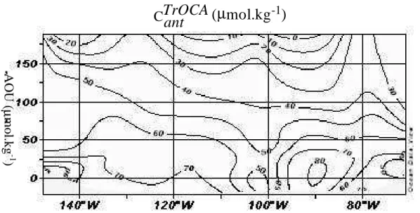
Printer-friendly Version Interactive Discussion a e b f c g d h CT(µmol.kg-1) AT(µmol.kg-1) σθ(kg.m-3₎ TrOCA ant C µmol.kg-1 O₂(µmol.kg-1₎ Salinity θ(o_C₎ AOU (µmol.kg-1₎

Fig. 3. Vertical distribution of the physicochemical parameters and the anthropogenic CO₂

estimated with the TrOCA approach. (C_antTrOCA: (a) O₂(µmol kg−1), (b) AOU (µmol kg−1), (c) C_T (µmol kg−1), (d) σ_θ(kg m−3), (e), S, (f) θ (◦C), (g) A_T (µmol kg−1), (h) C_antTrOCA(µmol kg−1).

(22)

BGD

4, 1815–1837, 2007

Printer-friendly Version Interactive Discussion EGU

(

µ

m

o

l

.

k

g

-1

)

TrOCA

ant

C

A

O

U

(

µ

_m

o

l.k

g

-1

)

(23)

BGD

4, 1815–1837, 2007

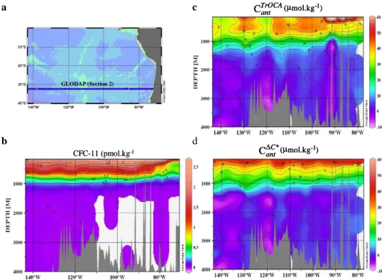
Printer-friendly Version Interactive Discussion a c b d GLODAP(section1) (µmol.kg-1₎ TrOCA ant CTrOCA(µmol.kg-1₎ ant CTrOCA(µmol.kg-1₎ ant C (µmol.kg-1₎ * C ant ∆ C C*(µmol.kg-1₎ ant ∆ C C*(µmol.kg-1₎ ant ∆ C CFC-11 (pmol.kg-1 CFC-11 (pmol.kg-1

Fig. 5. Vertical distribution on the Sect. 1 of the GLODAP data of the anthropogenic CO₂ esti-mated with the TrOCA approach. (CTrOCA_ant and the ∆C* approach (Cant∆C∗) and the anthropogenic tracer the CFC-11: (a) Location of the Sect. 1 of the GLODAP data, (b) CFC-11, (c) CTrOCA_ant , (d)

(24)

BGD

4, 1815–1837, 2007

Printer-friendly Version Interactive Discussion EGU a c b d (µmol.kg-1) TrOCA ant

CTrOCA_ant (µmol.kg-1)

C (µmol.kg-1₎ * C ant ∆ C C*(µmol.kg-1₎ ant ∆ C C*(µmol.kg-1₎ ant ∆ C CFC-11 (pmol.kg-1 CFC-11 (pmol.kg-1 GLODAP (Section 2)

Fig. 6. Vertical distribution on the Sect. 2 of the GLODAP data of the anthropogenic CO₂ esti-mated with the TrOCA approach. (CTrOCA_ant and the ∆C* approach (Cant∆C∗) and the anthropogenic tracer the CFC-11: (a) Location of the Sect. 2 of the GLODAP data, (b) CFC-11, (c) CTrOCA_ant , (d)