Developing software for compressed imaging transcriptomics

Developing Software for Compressed Imaging

Transcriptomics

by

Shahul Alam

B.S., Computer Science and Engineering

Massachusetts Institute of Technology (2020)

Submitted to the Department of Electrical Engineering and Computer Science

in partial fulfillment of the requirements for the degree of

Master of Engineering in Electrical Engineering and Computer Science

at the

MASSACHUSETTS INSTITUTE OF TECHNOLOGY

September 2020

© Massachusetts Institute of Technology 2020. All rights reserved.

Author . . . .

Department of Electrical Engineering and Computer Science

August 21, 2020

Certified by. . . .

Aviv Regev

Professor

Thesis Supervisor

Accepted by . . . .

Katrina LaCurts

Chair, Master of Engineering Thesis Committee

Developing Software for Compressed Imaging Transcriptomics

by

Shahul Alam

Submitted to the Department of Electrical Engineering and Computer Science on August 21, 2020, in partial fulfillment of the

requirements for the degree of

Master of Engineering in Electrical Engineering and Computer Science

Abstract

Modern-day biological experimentation often necessitates a scale of data that is exponen-tial with respect to the number of genes that are being measured, and this in turn leads to high latency and monetary cost during hypothesis testing. In addition to such practical constraints, some biological experiments are just physically infeasible due to fundamental limitations on the throughput of current technologies. However, because nearly all biological data are highly structured and can be described in terms of relatively few components, it is not necessary to measure each data point individually. Instead, using the framework of com-pressed sensing, it is possible to take advantage of this structure to gather the requisite data for an experiment while collecting only a fraction of the original number of measurements. In previous work, we have applied compressed sensing for the particular purpose of generating spatial gene expression profiles using fluorescence microscopy (i.e. imaging transcriptomics). In order to make this technique more accessible and user-friendly, we built CISIpy, an open-source software system that implements the pipeline’s computational aspects. This system is designed to enable efficient compressed sensing workflows that is highly portable across platforms and especially amenable to cloud computation. The end result is a well-tested, open-source software package replete with functionality, documentation and examples. Thesis Supervisor: Aviv Regev

Acknowledgments

First of all, I would like to thank my incredible research mentors during my time at MIT. To Aviv: thank you for offering me my first taste of research when I asked for it one day in Spring 2017 after 7.03 lecture; I was so inexperienced then, but thanks to my time with you, I was able to grow into the computer scientist that I am now. And to Brian: thank you for being an excellent mentor, an inspiring researcher and a good friend over the past three years. Despite my part-time availability and inconsistent work schedule, you always managed to guide me in the right direction, and I am eternally grateful for that.

To Mom, Dad and Shorna: I would not be here without you. Thank you for supporting me no matter what choices I make and no matter how hard life gets! I love you!

To Lauren: you are the OG inspiration and a dear friend, and your support has kept me going during the roughest of times. Please know that! To Mahi: thanks for being my in-tellectual comrade at MIT and serving with me in our mutual crusade against bad content and fake news; it’s truly been a pleasure. To Larry: you are a real homie, and I don’t know if I would have survived all those late nights in the main lounge without your company. To Andy: you’re such a great guy and a source of much mirth in my life, and I’m grateful to count you as a friend. To Austin: I hope you know that you’re like the brother I never had. And to 3E: thank you for being my second family, and for giving me a home away from home. I will be back to visit someday soon! Thank you all for supporting me along my journey and helping me grow every day.

Contents

1 Introduction 9

1.1 Introduction to Compressed Imaging Transcriptomics . . . 9

1.2 Background and Related Work. . . 11

1.2.1 Compressed Sensing in Biological Applications . . . 11

1.2.2 Compressed Imaging Transcriptomics . . . 13

1.2.3 Scientific Software Development . . . 14

2 Building a Software Suite for CISI 17 2.1 Design Choices . . . 17

2.1.1 Comparison of Implementation Options . . . 18

2.1.2 Deciding an Implementation . . . 19

2.2 Implementing an Image Preprocessing Module . . . 20

2.2.1 Working With Raw Microscopy Data . . . 21

2.2.2 Stitching . . . 22

2.2.3 Spotfinding . . . 24

2.2.4 Registration . . . 26

2.2.5 Segmentation . . . 27

2.2.6 Enabling Parallel Processing . . . 28

2.2.7 Developing Unit Tests . . . 32

2.3 Implementing a Compressed Sensing Module . . . 32

2.3.1 Developing Unit Tests . . . 34

2.3.2 Training . . . 34

2.3.4 Analysis . . . 35

2.4 Configuring CISIpy . . . 35

2.5 Distributing CISIpy . . . 37

2.5.1 Building a PyPI Package . . . 37

2.5.2 Building CISIpy Docker Images . . . 37

2.5.3 Building a WDL Workflow and Publishing to Terra . . . 38

2.6 Documenting and Maintaining the Code . . . 38

3 Discussion 41 3.1 Reflection on Implementation Challenges . . . 41

3.1.1 Instability of CISIpy Dependencies . . . 41

3.1.2 Obstacles to Software Development and Iteration . . . 43

Chapter 1

Introduction

1.1

Introduction to Compressed Imaging Transcriptomics

In the context of experimental biology, a key goal is scalability. From generating gene ex-pression profiles for tissue samples to sequencing genomes, there are many obstacles that hinder rapid hypothesis testing and scalability, such as the time required to conduct experi-ments, the monetary costs incurred by each experiment, or simply the difficulty of procuring a large selection of biological samples. Nevertheless, these experiments are important, be-cause they can serve to characterize identifying features of a cell (e.g. its type, state or environment), and thus can be used in critical applications ranging from diagnosing cancer to assessing a drug’s biological toxicity. As the number of such applications grows, the need for high-throughput experimental protocols will only increase. One way to improve through-put is multiplexing, which allows an experimentalist to obtain several measurements in a single batch. However, current multiplexing methods are still insufficient to handle the sheer amount of data (which scales with both the number of genes and number of cell lines under investigation) produced during genome-wide profiling experiments.

Compressed sensing offers a computationally principled approach to this problem. The theory behind compressed sensing prescribes an efficient sampling scheme for signals that are structured in some way - most often, we assume that the signal fits a sparse model. In particular, with such a model, we can reconstruct a 𝑘-sparse signal in 𝑛-dimensional space from just 𝑂(𝑘 log𝑛

increase throughput; indeed, compressed sensing can be utilized in parallel with multiplexing to further reduce the required number of measurements. In general, compressed sensing is expressed as a fitting problem that estimates the desired high-dimensional data using observed low-dimensional data:

𝑌 = 𝐴𝑋

In this formulation, 𝑌 are the compressed measurements, 𝐴 is the measurement matrix, and 𝑋 are the original measurements that we wish to recover. Further more, because 𝑋 may not necessarily be a 𝑘-sparse signal, we must decompose it using a basis in which it is sparse before we can apply compressed sensing. Thus, given a synthesis operator 𝑈 and the transformed measurements 𝑊 , we have the following formulation:

𝑌 = 𝐴𝑋 = 𝐴𝑈 𝑊

With this insight, we can measure the low-dimensional coefficients 𝑌 instead of measuring the high-dimensional data 𝑋 directly; this shift in modality is exactly what allows for a decrease in the required number of measurements.

In transcriptomics applications, we aim to measure signals that reveal the biological state of an organism - for example, we might seek to understand the relevance of a gene in causing a particular disease by measuring its RNA expression level in an ill patient’s tissue sample. For these applications, the aforementioned model is directly applicable: 𝑌 are composite measurements that consist of random linear combinations of gene expression signals, 𝐴 is a weight matrix that defines these composite measurements, and 𝑋 is the original gene expression measurement. Furthermore, 𝑈 is a learned dictionary of gene modules which captures the degree of co-regulation between genes, and 𝑊 expresses the original data in terms of these modules. We label this application of compressed sensing to the task of collecting biological data as compressive biology; we also use this as an umbrella term to encompass methods of decompressing that data and interpreting the results.

In previous work, our group has established the utility of compressive biology with respect to spatial profiling of gene expression. The goal of this work was to invent a new compressive modality by which biologists studying functional genomics can dramatically increase the scale

of their experiments. However, potential progress towards this goal is hindered by the lack of a reliable, modular software pipeline for compressed imaging transcriptomics. Such a pipeline can serve us twofold: 1) it facilitates rapid evaluation of alternative algorithms for decompression of composite measurements and 2) it aids in the distribution and accessibility of this technology. Thus, to this end, my thesis focuses on the following question: How can we design a scalable, maintainable, portable and well-tested software suite for compressed imaging transcriptomics?

1.2

Background and Related Work

1.2.1

Compressed Sensing in Biological Applications

Seminal work on compressed sensing established that it can be applied to any sampling problem given that 1) the data is sufficiently sparse in some basis and that 2) it is feasible to measure it using compressive modalities [4]. Often, biological data satisfy these constraints. For example, one of the earliest applications of compressed sensing involved increasing the throughput of magnetic resonance imaging (MRI), which is possible because this data is naturally compressible [19].

Further supporting the connection between compressed sensing and biological experimen-tation, it has been shown that gene expression data possesses exactly the aforementioned sparsity necessary to apply the technique [13]. For instance, previous studies have estab-lished that it is possible to discover high-confidence gene-phenotype correlations with shallow (low-coverage) RNA-sequencing, and this tendency to conserve precision while increasing throughput has been attributed to the inherent low-dimensionality of gene expression data. In order to further leverage this low-dimensional structure, some researchers have attempted to generate transcriptomic profiles based on just a small subset of “signature” genes - that is, genes believed to be the most influential in driving transcriptional programs [10][18]. This comes as an attempt to reduce the number of observations required to capture a snapshot of a cell’s profile. However, a drawback of this approach is that its scope is intrinsically tied to the functionality and abundance of the genes in its training set, and therefore

ex-pression levels for genes that are expressed at low frequencies are unlikely to be represented accurately.

Based on these observations, our group previously established the feasibility of applying compressive frameworks to gene expression data collection. Our first milestone was to apply compressed sensing to RNA-seq-like procedures [7]. We found that, using random compos-ite measurements, it is possible to recover gene expression measurements that are highly faithful to the expected data. This was accomplished using matrix factorization algorithms, such as sparse nonnegative matrix factorization (sNMF), in order to learn a dictionary of gene-to-gene interactions; using these learned relationships, we decompressed our composite measurements to produce measurements for individual genes. The fact that these composite measurements can be randomly chosen is important, as it allows us to incorporate all genes into our measurements, regardless of their expression frequency. Another tangent that was explored in this paper was the development of an algorithm for “blind compressed sensing” (compressed sensing without the use of a prelearned dictionary), which may remove the need for large training sets when applying compressed sensing.

The concept of composite measurements derives from the idea of group testing, which in turn can be thought of as a kind of "boolean" compressed sensing. The label "group testing" derives from the original application of this idea to disease-testing, in which multiple patients’ samples are mixed together in order to accommodate for scarce testing resources. Contextualized in the above compressed sensing formulation, this can be thought of as compressed sensing with the stipulation that 𝐴 and ˆ𝑋 (and therefore 𝑌 ) are all binary. Previous work has shown that, even in the presence of additive Bernoulli(p) noise (i.e. there is a 𝑝% chance of a test being a false positive), only O(𝐾 log 𝑁

1−𝑝 ) tests are required for an arbitrarily small average error probability [1]. Because of its potential for increasing testing efficiency and because of its robustness to noise, group testing continues to be explored as a useful tool in biology and medicine - for example, recent work has shown that group testing dramatically increases the efficiency of COVID-19 testing in resource-limited settings [8].

1.2.2

Compressed Imaging Transcriptomics

The goal of spatial profiling is to understand gene expression patterns across space. In these experiments, we produce pictures of RNA expression in a tissue sample: the brighter the intensity of a pixel in the image, the more RNA molecules have hybridized at that location in the image. Although this is a powerful data medium that contains much more information than classical gene expression measurements, spatial profiles are not usually employed due to the low throughput of current technologies for producing them. Thus, in our previous work, we implemented a compressed sensing pipeline to circumvent this problem and increase throughput. In this experiment, we used in situ hybridization chain reaction (HCR) across multiple rounds of imaging with composite probe sets to obtain spatial transcriptomes for mouse motor cortex tissue [6]. Within each round, we were able to obtain fluorescence signals over four channels. Between each round, we washed the sample to remove fluorescent probes from the previous round, added a new set of composite probes for the next round, replaced the sample onto the microscope; we then completed another round of imaging. In addition, we also imaged some individual genes directly to use as controls in order to verify our results during the experimental analysis.

To decompress these measurements, we developed the novel Composite In Situ Imaging (CISI) algorithm [9]. The first portion of the algorithm involves parsing signal from the microscopy data via a precise set of image processing steps; this is the preprocessing pipeline. After parsing these composite signals, we decompressed them using our sparse compressed sensing model, and we also analyzed the results by comparing to individually measured genes; this is the decompression pipeline. After applying this algorithm, we found that compressed sensing is indeed viable for spatial transcriptomics data, as we were able to recover spatial expression profiles for 37 genes using only 10 composite measurements - i.e. a 3.7x speedup - while maintaining a high correlation between the reconstructed images and the traditionally-measured images. Furthermore, because composite images do not require spot-level resolution, we were able to image at a magnification ∼ 10x lower than with non-compressive spatial profiing. Combined, these savings allowed us to reduce imaging time by an order of magnitude.

However, despite this exciting result, the compression ratio achieved was not enough to enable the desired scale of tissue profiling experiments - specifically, imaging of a whole mouse brain sample, and eventually imaging of a human brain. Fortunately, our preliminary work shows that it is possible to achieve an even higher compression ratio. Furthermore, it is possible to improve upon these results by applying compressed sensing to other aspects of the data - in particular, we can leverage 1) sparsity in the color space of the fluorescent probes used during tissue imaging and 2) sparsity in the pixel space of the images themselves in order to increase throughput by several orders of magnitude. Ultimately, we believe that the combination of these techniques can increase throughput by a factor of ∼ 25, 000, which is enough to make our proposed organ-scale expression profiling a feasible task.

1.2.3

Scientific Software Development

The problem of building high-quality software for scientific computing is one that has recently gained increased attention. This is especially true in the realm of computational biology, in which scientists and engineers alike often lack advanced training in software and program design [2]. The result is a legacy of unmaintainable, inscrutable codebases that are virtually impossible for an outsider to utilize. At the same time, the need for open-source software has never been more important in computational biology, as researchers seek to reproduce and quickly iterate upon previous work. Even as the researchers themselves become hyper-aware of this need, well-established institutions in computational biology lag behind in aiding this ambition, as until recently even influential publications such as Nature did not explicitly require authors to publish open-source, peer-reviewed code [15].

One tool that is aiding in the adoption of this open-source mentality among the com-putational biology community is the growing popularity of a now ubiquitous technology: cloud computing. In many modern experiments, cloud computing is an essential tool that enables scientific analyses that would otherwise be impossible to compute in a reasonable timeframe. For example, variant calling, ChIP-seq analysis and RNA-seq analysis have all been run at scale on the cloud [17]. This reliance on cloud computing has also informed soft-ware development patterns in computational biology, as programmers can take advantage of high-performance computing frameworks like MapReduce or Apache Spark. At the same

time, some experiments benefit from running partly on the cloud and partly on computing clusters in a hybrid framework [23]. In any case, it is clear that it is important to consider deployment in the cloud as an ultimate use case when designing scientific software.

Chapter 2

Building a Software Suite for CISI

2.1

Design Choices

The code for the prototype of CISI was first implemented and executed on the Broad In-stitute’s powerful computing cluster. While the Broad’s cluster is an excellent resource for quickly developing biological experiments that require high processing power and memory, it also discourages the use of software engineering best practices. This is, in fact, a common aspect of many scientific communities that use cluster-based computing for their research: maintainable, portable and user-friendly code is often sacrificed for the sake of reduced de-velopment time and rapid prototyping. However, in the past few decades, a combination of factors has contributed to a changing attitude towards writing good scientific code. In particular, the rise of cloud computing, the crossover between the software engineering and scientific research worlds and an influx of new technologies have all heralded a growing com-munal interest in writing quality software that can withstand the test of time. Due to these developments, there were several decisions to make before we could begin implementing the CISI software suite.

2.1.1

Comparison of Implementation Options

Programming Language

One of the first decisions was the choice of programming language in which to implement our application. While the original CISI experiment consisted of a collection of Bash and Python scripts, the majority of code in the microscopy software ecosystem is written in Java - most notably, ImageJ, an open-source application developed by the NIH for biomedical image processing, is implemented entirely in Java [25]. Thus, in making this decision, we compared the relative benefits of using Java versus Python. The main appeal of Java is its ability to integrate with existing software like ImageJ. Furthermore, the reason that ImageJ was implemented in Java was to take advantage of the Java Virtual Machine (JVM), which guarantees code portability by ensuring that Java code will have the same effect when executed on any operating system-hardware combination; this would be an excellent feature to inherit. On the other hand, Python has quickly become the research world’s most popular programming language, and as a result it boasts an oversized warehouse of open-source libraries for scientific computation that are under active development. This can largely be attributed to the relative ease of writing and iterating on Python code in comparison to code written in a more verbose language like Java.

Distribution Options

After packaging CISI, the crucial next step is distributing the software so that it is easy for collaborators to reproduce our work in a variety of computing environments. For Java applications, this entails creating a JAR file and publishing it to a remote repository like Maven. Similarly, we can publish Python packages on a repository like PyPI. One advantage of Python in this respect is that the default installation of Python comes with pip, a tool that retrieves packages from PyPI, whereas Maven’s package manager comes separate from the default Java installation. In either case, however, this sort of distribution is not enough to ensure reproducibility in all computing environments; to ensure such a degree of control over a user’s workspace, it is necessary to build a container.

runtime environment - e.g. they can bundle Python, Java and C++ packages and their dependencies at a single location. For CISI, we considered two container options: Docker and Singularity [21][16]. While Docker creates containers that are as isolated from the host machine as possible, Singularity is instead optimized for high-performance computing and favors integration with the host system instead. In addition, Singularity can actually run using images built for Docker - the reverse is not true. However, despite the fact that CISI certainly falls under the high-performance computing umbrella, Docker is much more widely-supported and popular than Singularity and thus it is easier to develop. Another development advantage is that Singularity is available on the Broad Institute’s cluster, but Docker cannot be installed due to the fact that it requires root access to the computing system.

This leads us to the final aspect of distributing CISI - publishing and deploying on cloud-based platforms. In recent years, the number of options for hosting and sharing com-putational workflows for biology on the cloud has proliferated. For example, two options are DNAnexus and Terra. DNAnexus is a decade-old company that enables customers to deploy and scale computational workflows, while Terra is a revent Broad Institute initiative that harbors similar ambitions while maintaining an open-source codebase and operating free-of-charge. Whereas DNAnexus supports using Amazon Web Services (AWS) and Azure as the computational backends for users’ workflows, Terra exclusively uses the Google Cloud Plat-form (GCP). Both platPlat-forms support using Docker images to start up cloud environments for workflows.

2.1.2

Deciding an Implementation

Ultimately, we chose a compromise between several options. To increase the usability of our application, we chose to primarily implement it in Python, a language which is well-known for being syntactically simple and otherwise beginner-friendly. The choice of Python also made it possible to rely on the rich repository of image processing Python libraries available on PyPI. From this choice, we also decided a name for our application: CISIpy. We decided that one necessary component to package CISIpy was a corresponding pip package, titled cisipy. In addition, due to the fact that CISI has complex dependencies that incorporate

multiple software systems written in a variety of programming languages, it was necessary to simultaneously implement a Docker image that would containerize these dependencies. We prioritized Docker over Singularity because there is more existing support for integrat-ing Docker into cloud workflows. This image is hosted on DockerHub and is available for public download at shahulalam/cisipy. We also built a Singularity image in order to pull the Docker image within the Broad’s computing environment; however, this image is not as stable as the Docker image and thus is not yet available for download. To further in-crease ease of use and scalability, the Docker image was incorporated into a Terra workflow; this workflow takes as input a configuration file (see Section 2.4) and microscopy data and outputs decompressed images, all within the Google Cloud environment. Although Terra is significantly less developed than some of its competitors, we decided to use it because it aligns with our open-source ambitions, and also because it is the cheapest option (free-to-use aside from GCP computing costs).

With these resources, there are now several options for running CISIpy, with varying degrees of configurability:

• Download the cisipy pip package and correctly install its non-Python dependencies (e.g. ImageJ, CellProfiler and various APT packages), and write a Python script that uses cisipy functionality.

• Pull the shahulalam/cisipy Docker image from DockerHub, and write a Python script that uses cisipy functionality; run on local computing resources.

• Create a Google Cloud billing account, upload your data to a Google Cloud bucket, import the Terra workflow and run the workflow in the cloud.

2.2

Implementing an Image Preprocessing Module

The initial computational aspect of the CISI procedure is the preprocessing of raw micro-scope data prior to its decompression. Converting this raw data into a viable format for understanding spatial transcriptomics patterns is a non-trivial task. For this purpose, we designed and implemented a preprocessing submodule for the cisipy pip package, which

takes as input a raw Nikon microscope file with composite imaging data from a tissue sample and outputs a format that can be easily decompressed using compressed sensing algorithms. The following is a chronological list of steps for preprocessing the spatial transcriptomics data:

1. Stitching the microscope fields-of-view into a single image with ImageJ. 2. Highlighting only cell-sized spots in the tissue sample with Starfish.

3. Registering (i.e. aligning) images acquired across multiple rounds of in-situ HCR imaging.

4. Segmenting only cells from the images with CellProfiler.

2.2.1

Working With Raw Microscopy Data

The first hurdle involved in handling imaging transcriptomics data is that it is measured by a microscope, and as such is stored in a microscope-specific format. These formats are not easily readable or writable - for example, there is no native Python library that can interface with these data formats. Indeed, until recently it was not possible to process these files except via Java, since this has been the language-of-choice for the biological image processing community for some time; this can largely be attributed to the success of ImageJ. Thanks to the recent efforts of the community, there now exists nd2reader, an open-source library that make it possible to interact with ND2 files (which are a file format used by Nikon microscopes) in Python. Unfortunately, while nd2reader makes it easy to extract image data from these files, it does not parse the experimental metadata in a convenient format. Indeed, this metadata is the most distinguishing feature of these unique file formats, and it must be preserved in order to properly inform downstream preprocessing steps.

For this reason, we turn to Bio-Formats, a Java library that can parse both imaging data and metadata from a large selection of microscope file formats, including ND2. Fortunately, there is a Python binding of Bio-Formats (python-bioformats) that serves as a wrapper around this library and allows us to integrate it into CISIpy. python-bioformats relies on javabridge, a package that starts the JVM from Python and thereby is able to call

upon Bio-Formats’ Java code. Bio-Formats reads ND2 metadata and converts it into OME-XML, a metadata format created by the Open Microscopy Environment (OME) consortium explicitly for the purpose of standardizing microscopy data [12]. Combining this with the tifffilelibrary, we can convert the input ND2 files to OME-TIFF files, an enriched TIFF-like format that stores metadata as OME-XML. This functionality is encapsulated in a CISIpy submodule (cisipy.preprocessing.nd2_utils).

2.2.2

Stitching

The next step is to convert the microscopy data into a single image representing a transcrip-tomic snapshot of the sample. This process is called stitching, as it requires that multiple fields-of-view (FOVs) produced during the imaging are "stitched" together (Fig. 2-1). In order for any stitching algorithm to succeed, there are two important prerequisites: 1) we need the relative position in XY-coordinates of the microscope head as it imaged each par-ticular FOV and 2) each FOV must overlap slightly with its neighbors to ensure that there are no gaps while imaging the sample. We need both requirements because the microscope tends to drift as it images different FOVs, and thus XY-coordinates are not precise enough to correctly stitch the data.

There were several options to support stitching. The first, most native option was to im-plement an algorithm in Python that uses cross-correlation minimization to find the optimal shift between two FOVs, perhaps utilizing a popular library like OpenCV or scikit-image. However, after initial prototyping with such algorithms, we found that they did not per-form well for our sparse microscopy images. Instead, we turned to ImageJ, which ships with implementations of stitching algorithms specifically tailored to microscopy.

We decided to use Fiji, a version of ImageJ that includes many useful plugins [24]. One of the default plugins that Fiji ships with a "Stitching" plugin. This plugin was first created in 2009 and has been continuously updated since then, and has proven sufficient in many applications [22]. However, in 2018, a very robust and performant stitching algorithm optimized for large datasets was introduced in the form of the "BigStitcher" ImageJ plugin [14]. Although BigStitcher is perhaps less well-established than the Stitching plugin, our initial tests showed that it performed better on our data, so we opted to incorporate it into

our workflow.

In order to use BigStitcher in the cisipy Python package, we used pyimagej a wrapper in beta development that allows us to access ImageJ functionality in Python. pyimagej uses pyjnius, a package similar to javabridge that invokes the JVM to run ImageJ from Python. One final hurdle is that ImageJ and BigStitcher were originally designed to be used with a graphical user interface (GUI); in order to run them in "headless" mode (without a GUI), we took advantage of ImageJ’s macro-scripting language, which allows us to reproduce GUI inputs from a script. This script is bundled as a resource in the cisipy PyPI package.

Figure 2-1: An example of stitching eight FOVs from a nuclear DAPI stain into a coherent image using ImageJ’s BigStitcher. Each of the eight FOVs slightly overlaps its neighbors, allowing the stitching algorithm to correct translate the tiles into the correct locations. Notably, there is an error with the stitching of the top-right tile which is obvious even to the human eye - unfortunately, even the BigStitcher algorithm is not always successful.

2.2.3

Spotfinding

After obtaining a stitched image, we begin extracting signal from it. We begin by isolating "spots" in our images of significant size, which helps us distinguish transcriptomic signal from noise/artifacts that arise during image acquisition. This is an appropriate approach because the fluorescent pixels in our data should be clustered within cells due to the nature of the , and thus they naturally form spots; any other fluorescence patterns can be ignored. Therefore, after isolating spots, all other pixels can be "zeroed-out" to black (Fig. 2-2).

We use starfish, a Python library for processing spatial transcriptomics data, for spotfinding. starfish wraps scipy’s find_peaks function and allows us to detect spots

of different sizes from a z-stack of image slices. In CISIpy, we create a starfish pipeline that finds small (2-10 pixel radius) and large (5-100 pixel radius) spots and isolates them. In this step, we also flatten the image z-stack into a 2D image by taking the maximum of each pixel along the z-axis. We chose starfish because it is a tool very specific to our application - spot-finding in spatial transcriptomics data. This is despite the fact that the package is still in beta development; indeed, as the software matures, we may replace other aspects of the CISIpy preprocessing pipeline with starfish functionality.

Spotfinding functionality is available under the submodule cisipy.preprocessing.spotfinder.

Figure 2-2: An example of finding and isolating spots from a stitched composite image. This has the effect of nullifying much of the noise that is inherent in the imaging process; it also helps remove artifacts that arose during stitching, such as artificially dark patches of zero-fluorescence.

2.2.4

Registration

Because we acquire spatial transcriptomics data across multiple rounds of imaging, we must register, or align, the data obtained across multiple rounds (Fig. 2-3). This is because the sample is washed and displaced from the microscope stage between each round, and thus the sample is positioned slightly differently between rounds. We use a phase cross-correlation minimization algorithm from the scikit-image library to obtain the optimal XY shifts that align all rounds of imaging, which allows us to correctly compare images between rounds. After registration, there are inevitably pixels with zero fluorescence introduced near the borders of the image; instead of keeping these artifacts, we simply crop all of the registered images to the same dimensions so that they exclude these black pixels.

Figure 2-3: An example of registering nuclear DAPI stains from two different rounds. In both images, two DAPI stains from different rounds of imaging are overlapped, with 50% transparency applied to each image. After registration, the result is a much closer alignment between DAPI stains from different rounds, which is demonstrated by the increased overlap in the images and the decreased blurriness.

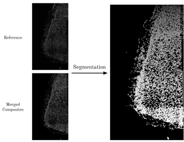
2.2.5

Segmentation

To reliably compare transcriptomic profiles captured across multiple rounds of imaging, it is necessary to do more than just spotfinding - we must identify actual cells in our sample. The task of identifying pixels that belong to cells is known as cell segmentation, and it is a difficult problem with many variants (Fig. 2-4). One of the most popular tools for cell segmentation is CellProfiler, an open-source software system for high-throughput cell image analysis [5]. CellProfiler is highly configurable and offers a GUI interface that is ideal for biologists without any coding experience - which in part explains its popularity. However, recent work has resulted in deep learning models for cell segmentation (e.g. UNet and DeepCell) that offer an alternative to CellProfiler [26]. Indeed, it has been shown that these deep learning methods perform better than CellProfiler for the task of nuclear segmentation - that is, identifying the pixels that comprise the nucleus of each cell [3].

Ultimately, we chose to use CellProfiler for our segmentation step. This is because, while deep models offer marginally better performance than CellProfiler’s methods, they also require more resources to run. For example, in order to use deep cell segmentation models effectively, they must be retrained and tailored to the dataset on which they are being applied, and this in turn requires a human to label cells in the training data. In addition, deep models consist of many parameters that must be downloaded and stored on disk space, and they are difficult to efficiently bundle in a Python package or Docker container. Thus, CellProfiler was chosen for ease-of-implementation.

There were two main obstacles to incorporating CellProfiler into CISIpy: 1) CellProfiler was originally implemented in Python 2, which is incompatible with CISIpy’s use of Python 3 and 2) CellProfiler is optimized for interactive data processing in which a human feeds parameters to the pipeline via a GUI. To resolve these issues, we used the latest development version of CellProfiler (version 4.0.0rc9), which is a beta release of CellProfiler 4. This new version supports Python 3 as well as a headless mode for batch operation of CellProfiler without a GUI.

We provide two images as inputs to the CellProfiler segmentation algorithm. The first is a reference nuclear stain image from one of the rounds in the sample - the particular round

that is chosen is not important, since these images should be the same for each round after the previous preprocessing steps. The second image is obtained by merging all the composite images via a max filter - this provides a summary of RNA expression for all the genes in our experiment in the image. CellProfiler uses these inputs to segment cells using a watershed algorithm. After obtaining segmented cell masks, we save a mask for each cell in a sparse matrix format. We then integrate the pixel intensities of each cell by taking the dot product of each mask with every image, producing a vector with (# of cells) entries for each image; this is the final output of the preprocessing pipeline.

Figure 2-4: An example of segmenting cells from an image. The CellProfiler segmentation algorithm takes as input two images: . The picture on the right is Each segmented cell is saved as a sparse mask.

2.2.6

Enabling Parallel Processing

Throughout the preprocessing steps, there are multiple opportunities for parallel processing. With parallel processing, we can run some of the necessary computations at the same time,

thereby decereasing the overall "wall-clock" time required. Although it is true that each step of the preprocessing pipeline must be performed sequentially, we can easily parallelize across the multiple samples that we are processing or even across the multiple rounds of imaging that must be processed for a single sample. In fact, without parallelism, it is infeasible to complete these preprocessing steps in a reasonable amount of time, so it is critical that we are able to do this.

There are two approaches we can take to preprocessing: 1) parallelizing a job across multiple cores on a single machine, or 2) distributing subtasks across multiple computing instances on a cloud platform, and then merging the results together. We opted for the first approach, as this is the most portable option that can be easily used without modification on non-cloud platforms. While augmenting our code to be amenable to concurrent execution, we prioritized changing keeping the interface to the module as simple as possible, so that the method of parallelization could be black-boxed by users (Listing 1). Below, we detail the techniques by which we enabled parallelization for each of the cisipy.preprocessing submodules as well as any limitations that we encountered in the process.

stitcher

Using pyimagej, it is easy to parallelize stitching across multiple rounds of imaging by calling on the JVM to create a separate thread for each job. This is because Java has first-class multithreading support, which means that it can spawn separate threads that compete for execution time on a machine. However, it is slightly more difficult to hierarchically parallelize stitching across multiple samples and rounds at the same time. Because of Python’s global interpreter lock (GIL), creating multiple threads to process each sample (e.g. by using the multithreading library) is not a viable option due to Python’s global interpreter lock (GIL), which essentially stipulates that CPU-intensive threads must not run at the same time. However, since the JVM can only be initialized once per thread, it is also not possible to use Python’s multiprocessing module to accomplish this. Thus, this second tier of parallelization is currently unimplemented.

spotfinder

Since starfish is implemented entirely in Python, it is easy to hierarchically parallelize spotfinding across both samples and rounds using the multiprocessing library - that is, we can spawn a process for each sample, and each of these processes can spawn a child process for each round of imaging within the sample.

register

During registration, we can easily parallelize across multiple samples by using multiprocessing; however, since the registration process uses information from all rounds of imaging, it is not possible to parallelize across multiple rounds without a finer-grained approach. At the same time, registration is the least time-consuming aspect of the preprocessing pipeline, so this is a low-priority enhancement.

segmenter

The key complication that arises when parallelizing cell segmentation is running CellProfiler concurrently. Although CellProfiler has native support for pipelines on individual image sets in parallel via the GUI, there is no option to do this in headless mode. However, this feature is under active development, and thus will be incorporated into CISIpy when it is available.

# Sequential function for a preprocessing step; processes each imaging # round one after another

def sequential_preprocessing_task(sample) sample_name = sample["name"]

rounds = sample["rounds"]

for round_index, imaging_round in enumerate(rounds, start=1): preprocess_round(sample_name, round_index, imaging_round) ...

# Parallelizable preprocessing function with a `parallelize` parameter; # allocates multiple processes for multiple rounds

def parallelizable_preprocessing_task(sample, parallelize=0): sample_name = sample["name"]

rounds = sample["rounds"] processes = []

for round_index, imaging_round in enumerate(rounds, start=1): if parallelize > 0:

process = mp.Process(

target=preprocess_round,

args=(sample_name, round_index, imaging_round) )

process.start()

processes.append(process) else:

preprocess_round(sample_name, round_index, imaging_round)

# Wait for child processes to terminate before quitting

for process in processes: process.join()

Listing 1: A pseudocode example of refactoring preprocessing code to execute in parallel using Python’s multiprocessing, with parallelization-related code highlighted in cyan. A key feature is that the function’s interface does not change; the user can run a non-parallelized version of the function while being completely oblivious to the parallelize parameter.

2.2.7

Developing Unit Tests

A critical component of any software development endeavor is comprehensive unit testing, i.e. tests that verify the functionality of individual units of code within the software. For CISIpy, it makes most sense to define these "units" according to the various steps in the CISI pipeline. For the preprocessing submodule in particular, it is natural to test the stitcher, nd2_utils, spotfinder, register and segmenter functions separately. An initial difficulty with developing these unit tests was that the initial CISI experiment generated microscopy files that were very large in size, and thus it was difficult to use them to create tests that could be computed in a reasonable timeframe. However, after converting the raw ND2 files into OME-TIFF files (see Section2.2.1), it was possible to subset this data and develop tests on such excerpts.

We curated three test datasets:

1. small_test: Four fields-of-view in a single column, five rounds of imaging

2. medium_test: Eight fields-of-view arranged in two columns, five rounds of imaging 3. large_test: 32 fields-of-view, five rounds of imaging

The input data and expected output data for each of these tests can be downloaded from a public Google Cloud bucket; see the documentation for details.

2.3

Implementing a Compressed Sensing Module

After preprocessing the microscopy imaging data into a vector per each composite image, the next step is to decompress the data using our compressed sensing model. For this purpose, we implemented a decompression submodule for the cisipy pip package, which takes as input the vectors produced by preprocessing and returns a decompressed vector for each gene that was involved in the original experiment.

Recall that our compressed sensing problem can be expressed by the following formula-tion:

Here, 𝑌 are the composite measurements and 𝐴 is the binary weight matrix that combines the individual gene measurements to produce these composite measurements; 𝑋 are the individual gene measurements that we wish to obtain from decompression, and ˆ𝑋 are the approximate decompression results that we actually obtain from our algorithm. Note that in the absence of noise it is possible to achieve 𝑋 = ˆ𝑋.

To apply compressed sensing, the data to be decompressed must be sufficiently sparse under some representation. Thus, before decompressing, we must learn a basis from prior gene expression data in which our transcriptomics data is actually sparse. This basis, or "dictionary", can be used to analyze the individual gene measurements as below:

𝑋 = 𝑈 𝑊 ≈ 𝑈 ˆ𝑊 = ˆ𝑋,

where 𝑈 is the gene dictionary and 𝑊 are the analysis coefficients of the gene measurements in this sparse representation. We can interpret 𝐴𝑈 = 𝐹 as a composite analysis operator that transforms sparse coefficients 𝑊 into composite measurements 𝑌 . Under the assumptions of this model, the following 𝑙1-penalized optimization problem gives us a solution for ˆ𝑊:

min ^ 𝑊 ∈R𝑝×𝑛 ⃦ ⃦ ⃦ ˆ 𝑊 ⃦ ⃦ ⃦ 1 s.t. ⃦ ⃦ ⃦𝑌 − 𝐹 ˆ𝑊 ⃦ ⃦ ⃦< 𝜆,

where 𝑝 is the number of modules in the gene dictionary, 𝑛 is the number of segmented cell data points and 𝜆 is a parameter that enforces that ˆ𝑊 ≈ 𝑊

The following is a list of the steps involved in the decompression pipeline:

1. Learning a set of gene modules using the SMAF algorithm.

2. Decompressing the composite vectors using the learned gene modules.

3. (optional) Analyzing decompressed results by comparing them to expression vectors of individually measured genes.

2.3.1

Developing Unit Tests

Just as we had three unit tests for the preprocessing pipeline, we have three unit tests for the decompression pipeline derived from the outputs of those previous tests:

1. small_test: Four fields-of-view processed into expression vectors of length (# of cells) for ten composite measurements

2. medium_test: Eight fields-of-view processed into expression vectors of length (# of cells) for ten composite measurements

3. large_test: 32 fields-of-view processed into expression vectors of length (# of cells) for ten composite measurements

As the number of FOVs increases, so does the number of cells segmented during the preprocessing pipeline.

2.3.2

Training

Before we can decompress, we must learn the gene dictionary 𝑈. The dictionary is trained using gene co-expression data acquired prior to the experiment. In the current implemen-tation, the input data must be single-cell RNA-sequencing (scRNA-Seq) data, and must include co-expression data for every gene that is part of a composite measurement. We use the sparse module activity factorization (SMAF) algorithm, a matrix factorization algorithm specifically designed to produce sparse, non-negative modules for biological data [7]. The code for training is available under the cisipy.decompression.training submodule.

2.3.3

Decompressing

In order to decompress, we first take the dot product of 𝐴 (the binary measurement matrix determined by the design of the CISI experiment) and 𝑈 (the learned gene module dictio-nary from the training step) to obtain our composite operator 𝐹 . We then use SPAMS (SParse Modeling Software), a C++ library with Python bindings that efficiently imple-ments a variety of sparse decomposition algorithms [20]. In particular, we use an

imple-mentation of the LARS algorithm, which very efficiently implements the lasso optimiza-tion method [11]. Once we have obtained ˆ𝑊 from the output of this optimization, we then multiply by 𝑈 to get our decompressed measurements ˆ𝑋; these are the final, de-compressed results. The code for decompressing the measurements is available under the cisipy.decompression.decompresser submodule.

2.3.4

Analysis

In the original CISI experiment, in addition to the collection of compressed mesurements, we also imaged some genes normally, using non-compessive modalities. These data serve as controls, and we can compare the decompressed measurements produced by CISI to the normally measured genes to verify our results. This is an optional step, since this type of analysis is only available if such control measurements were taken during the original imaging, and may not be necessary if the user is already confident that CISI will work for their samples. Thus, we do not believe that most users will use this functionality; nevertheless, it is included under the cisipy.decompression.analyzer submodule.

2.4

Configuring CISIpy

Due to the complexity of the CISI procedure, there are many configuration details and hyperparameters that must be specified in addition to the microscopy data in order to successfully run the pipeline.

To satisfy these constraints, we chose to create a simple TOML configuration language. TOML, which stands for "Tom’s Obvious, Minimal Language", is a simple configuration file format with plain-language syntax; thus, it is much more suitable for our purposes than YAML or INI, two other popular formats. With this language, it is easy to specify resources necessary to run CISIpy (e.g. a path to a local installation of ImageJ) as well as to add new rounds of imaging data to the experiment. Listing 2is an example of such a config file used during development of CISIpy. The configuration file is flexible in the sense that certain information can be omitted if one is only executing a part of the pipeline. A more detailed guide to writing such a configuration file is available in the documentation.

title = "cisipy_configuration"

workspace_directory = "medium_test"

data_directory = "data"

path_to_fiji="/opt/fiji/Fiji.app"

# Example entry for single tissue with multiple rounds of CISI imaging

[[samples]] name = "tissue1" [[samples.rounds]] filename = "D6_round1" reference_channel = 0 composite_channels = [1, 2, 3]

channels = ["DAPI", "Composite_6", "Composite_7", "Composite_2"] [[samples.rounds]]

filename = "D6_round2"

reference_channel = 0

composite_channels = [1, 2, 3]

channels = ["DAPI", "Composite_8", "Composite_9", "Composite_5"] [[samples.rounds]]

filename = "D6_round3"

reference_channel = 0

composite_channels = [1, 2, 3]

channels = ["DAPI", "Composite_0", "Composite_4", "Composite_1"] [[samples.rounds]]

filename = "D6_round4"

reference_channel = 0

composite_channels = [1, 3]

channels = ["DAPI", "Composite_3", "Ndnf", "Composite_10"] [[samples.rounds]]

filename = "D6_round5"

reference_channel = 0

channels = ["DAPI", "Vtn", "Csf1r", "F3"]

###

# Add more samples below by copying the syntax above! ###

2.5

Distributing CISIpy

As aforementioned, there are several methods of deploying CISIpy; here we discuss the process of implementing each method.

2.5.1

Building a PyPI Package

We began by building the cisipy module as a pip package. This involves creating a PyPI account, specifying Python dependencies on which the cisipy installation depends, specifying a minimum Python version (we chose Python 3.7) and specifying a license for the software (we chose the MIT license). The package homepage is available at https: //pypi.org/project/cisipy/, and can be installed on the command line with pip install cisipy.

Although cisipy has several large Python dependencies, the package itself is relatively lightweight; it is ∼ 50 kilobytes in size. This is because there is only source code in the package; test data is hosted on Google Cloud and must be downloaded separately.

2.5.2

Building CISIpy Docker Images

The next step was to build a Docker image that included CISIpy’s dependencies. While the cisipy pip distribution is able to specify Python dependencies, it is not able to indicate other dependencies (e.g. Fiji and CellProfiler). Thus, in addition to installing the cisipy package within the Docker image, we also explicitly install all other software that is neces-sary to run CISIpy. Furthermore, in anticipation of the Terra use case, our image inherits from a Terra-specific base image. This is necessary in order to run CISIpy on the cloud platform. Finally, we distributed the image by uploading it to DockerHub. One important performance consideration that arises when building Docker images is the size of the build. Our DockerHub image is 2 gigabytes in size, which is by all considerations excessively large. Although it is not a priority because this size is dwarfed by the size of the input data for a single CISI experiment, we would like to optimize this image size in the future.

2.5.3

Building a WDL Workflow and Publishing to Terra

Docker allows us to create a stable environment in which we can run CISIpy, but there is still some work to be done to properly run a CISI experiment on a set of input data with this image. To further reduce user friction, we created a workflow using the Workflow Description Language (WDL). WDL is maintained by the OpenWDL community and allows one to build a data processing workflow by specifying inputs, outputs, and a computing environment while running on a variety of platforms - e.g. Terra. Our workflow runs a Python script that calls CISIpy on input composite imaging data stored in Google Cloud; the outputs of the workflow are also stored on Google Cloud. The workflow WDL is available on GitHub, and it has also been published on Terra.

2.6

Documenting and Maintaining the Code

In order to guarantee maintainability of the CISIpy codebase, it is essential that the code is properly documented and easy to understand. For these purposes, we adhered to Google’s Python styleguide, which provides strict guidelines for writing straightforward, well-documented code. For example, the styleguide requires docstrings for every function in the codebase. In addition, the styleguide strongly recommends using Python 3’s function annotations to pro-vide type hints. These annotations allow developers to check that their functions pass the right types of data to each other without running any tests, which is especially powerful for a language like Python that lacks static type-checking. Although writing and maintaining such well-decorated code is a formidable time investment, it is vital to ensure that the software does not slowly deteriorate in quality and usability over time. Furthermore, we use Sphinx, a tool that converts markup language to PDF, HTML and other viewer-friendly formats, to automatically generate human-readable documentation for CISIpy from the source code (Fig. 2-5). This documentation is available at https://cisipy.readthedocs.io.

def stitch(input_directory, input_filename, output_directory, imagej_instance):

"""

Use the BigStitcher plugin to stitch together the series at input_filepath. See Fuse.ijm for the ImageJ macro code.

Args:

input_directory (Union[str, pathlib.Path]):

Directory in which input microscopy file is located. input_filename (str):

Name of microscopy file (excluding file extension). output_directory (Union[str, pathlib.Path]):

Directory in which to output stitched images, imagej_instance (imagej.ImageJ):

An ImageJ instance. Returns:

A handle on the Java process that is completing the stitching job. This is useful for keeping track of concurrent stitching jobs. """

# Formatting arguments correctly for ImageJ macro code

output_directory = str(output_directory) input_directory = f'{input_directory}/'

args = imagej_instance.py.to_java({

'basePath': input_directory,

'filename': input_filename,

'fusePath': output_directory })

stitching_job = imagej_instance.script().run(

"macro.ijm", STITCHING_MACRO, True, args ) return stitching_job

(b) Auto-generated documentation

Figure 2-5: An example of documentation automatically generated from the CISIpy source code using Sphinx. Sphinx automatically parses docstrings that adhere to Google’s python style guide and generates documentation for them.

Chapter 3

Discussion

3.1

Reflection on Implementation Challenges

In implementing CISIpy, we encountered many challenges that hindered the software engi-neering process and increased development time. By learning from these challenges, it will be easier to mitigate them in future projects.

3.1.1

Instability of CISIpy Dependencies

The first challenge was learning to manage complex dependencies that arose from working with external software in various degrees of health (e.g. some dependencies were installed from the "bleeding edge" of development, while others are soon-to-be deprecated software packages). Ensuring that all of these dependencies can coexist in one environment was non-trivial, and in the future it would be best to make this system of dependencies more stable. Below is a list of instabilities in CISIpy along with potential patches for the future:

• python-bioformats. This package is very buggy and poorly maintained; in addition, its maintainers have indicated that it will be deprecated in the near future. We use python-bioformatsto parse metadata from ND2 files into OMEXML, so the ideal fix would be to use a different library (or write our own code) to accomplish this and drop the python-bioformats dependency altogether.

• javabridge is incompatible with pyjnius. Because both libraries invoke the JVM from a Python process, they cannot be initialized within the same Python script; thus,

• tifffile. While this package is very functional and well-tested, it is still in beta development, and it is continuously receiving updates. It would be prudent to upgrade the package when a stable release is announced.

• CellProfiler. CellProfiler was initially designed to work for Python 2.x. In order to use CellProfiler with Python 3.x, it was necessary to install the most recent development version of the software: v4.0.0rc9. This was installed from the source, which can be found on GitHub. However, it is certainly still buggy - indeed, we discovered some bugs while attempting to install and use it - and it will be imperative to upgrade this dependency when a stable release is available.

• Terra. Terra is still in the beta stage of development, and as such its API and interface are liable to change as development continues. For example, while building our Docker image for CISIpy, we pulled from a Terra base image to ensure that our image would be compatible with Terra’s interactive mode. However, as Terra evolves, it may change its Docker image requirements, which could potentially requiring rewriting the Dockerfile for our image and/or pulling from a different base image.

• pyimagej. While ImageJ and Fiji are well-established software, the Python wrapper pyimagej is in beta development, and there are some unresolved issues with using it (e.g. combining Python multiprocessing with Java threading during parallel pro-cessing). Fortunately, this dependency is automatically tracked by pip, so the most up-to-date pyimage version is installed by default along with cisipy.

One benefit of working with these unstable dependencies, however, is that it pushed us to abstract as much of CISIpy’s functionality as possible into black-boxable units of code so that updating these dependencies in the future would not require completely overhauling CISIpy’s structure. As expected, this demonstrates the importance of developing meaningful abstractions when designing robust software.

3.1.2

Obstacles to Software Development and Iteration

There were many obstacles that hindered the actual process of writing and testing CISIpy code. The first stumbling block was simply the massive size of the input data for a typical CISI experiment. The total size of the microscopy data for a single experiment is several hundreds of gigabytes in size, and the obscure nature of microscopy file formats made it difficult to develop appropriately-sized miniature tests from this data; see Section 2.2.1 for details on how this was accomplished. Even after overcoming this initial hurdle, there were other difficulties. For example, because the prototypical CISI experiment was run on the Broad Institute’s computing cluster, development of CISIpy began in that environment. However, from that point forwards, it was actually necessary to develop CISIpy in several different environments, as each environment had some shortcomings that were difficult to circumvent. Below is a summary of the problems entailed by each environment:

• The Broad computing cluster. While this environment provides an abundance of com-puting resources, it is also restrictive in that users do not have root access to the operating system on which they work. Thus, it was difficult to install and test depen-dencies for CISIpy, which often assume that the user has root access during installa-tion. In addition, it is impossible to use Docker, since Docker requires root access to the filesystem.

• Local computing resources. Because of the requirement for root access to use Docker, the entirety of the Docker development process was performed on a personal MacBook Pro laptop. This included editing Dockerfiles, building the resulting Docker images, and even testing the images’ functionality. There were two main disadvantages to this environment: 1) network data transfer speeds on a home network are much lower than those on a high-performance computing cluster 2) using private hardware leads to the developer bearing the cost of each test computation personally.

• The Google Cloud Platform (GCP), utilized via Terra. This option is somewhat a compromise between the previous two, as we can use a Docker image to initialize the environment with all of CISIpy’s dependencies while maintaining access. However,

using the cloud has its own limitations. For example, Terra is primarily designed for non-interactive workflows. Although there is an interactive terminal mode that can be used, the interactive runtime will enter a "paused" state after some time, so it is impossible to interactively test code that takes some time to run. In addition, because Terra uses GCP, there is an additional cost for every hour of computation run on it.

3.2

Future Work

In order to maintain the quality of CISIpy, there are both engineering and scientific goals that must be achieved in the future. On the software side:

• Use GitHub as an issue tracker to find and resolve bugs. As more researchers install and run CISIpy, there will inevitably be bugs that they discover. By promoting the project’s GitHub repository as the primary location to report bugs, we can aggregate and respond to issues in the CISIpy codebase as they arise.

• Optimize Singularity image to provide an alternative to Docker. Building a Singularity image based on our Docker image is a simple way to increase the set of use cases with which CISIpy is compatible - for example, although the Broad computing cluster cannot run Docker due to security constraints, it can run Singularity. This is the case for many high-performance computing (HPC) clusters,

With respect to improving the CISIpy algorithm:

• Working with 3D voxels instead of 2D pixels. In the current implementation, the z-stacks of images captured by the microscope are flattened via a max filter after the spotfinding step. However, this erases some information that would probably enable more accurate decompression.

• Using deep learning models for image segmentation. Currently, we use heuristic-based algorithms from CellProfiler to segment cells from the microscopy data. However, state-of-the-art cell segmentation models are based on neural networks, and thus it would be of interest to see if such models would be more performant on our data.

Bibliography

[1] George K. Atia and Venkatesh Saligrama. Boolean compressed sensing and noisy group testing. IEEE Transactions on Information Theory, 58(3):1880–1901, Mar 2012. [2] Susan M. Baxter, Steven W. Day, Jacquelyn S. Fetrow, and Stephanie J. Reisinger.

Scientific software development is not an oxymoron. PLOS Computational Biology, 2(9):e87, Sep 2006.

[3] Juan C. Caicedo, Jonathan Roth, Allen Goodman, Tim Becker, Kyle W. Karhohs, Matthieu Broisin, Csaba Molnar, Claire McQuin, Shantanu Singh, Fabian J. Theis, and et al. Evaluation of deep learning strategies for nucleus segmentation in fluorescence images. Cytometry Part A, 95(9):952–965, 2019.

[4] Emmanuel J. Candès, Justin K. Romberg, and Terence Tao.

Sta-ble signal recovery from incomplete and inaccurate measurements.

Communications on Pure and Applied Mathematics, 2006.

[5] Anne E. Carpenter, Thouis R. Jones, Michael R. Lamprecht, Colin Clarke, In Han Kang, Ola Friman, David A. Guertin, Joo Han Chang, Robert A. Lindquist, Jason Moffat, and et al. Cellprofiler: image analysis software for identifying and quantifying cell phenotypes. Genome Biology, 7(10):R100, Oct 2006.

[6] Harry M. T. Choi, Maayan Schwarzkopf, Mark E. Fornace, Aneesh Acharya, Geor-gios Artavanis, Johannes Stegmaier, Alexandre Cunha, and Niles A. Pierce. Third-generation in situ hybridization chain reaction: multiplexed, quantitative, sensitive, versatile, robust. Development, 145(12), Jun 2018.

[7] Brian Cleary, Le Cong, Anthea Cheung, Eric S. Lander, and Aviv Regev. Efficient generation of transcriptomic profiles by random composite measurements. Cell, 2017. [8] Brian Cleary, James A. Hay, Brendan Blumenstiel, Stacey Gabriel, Aviv Regev, and

Michael J. Mina. Efficient prevalence estimation and infected sample identification with group testing for sars-cov-2. medRxiv, page 2020.05.01.20086801, May 2020.

[9] Brian Cleary, Evan Murray, Shahul Alam, Anubhav Sinha, Ehsan Habibi, Brooke Si-monton, Jon Bezney, Jamie Marshall, Eric S. Lander, Fei Chen, and Aviv Regev. Com-pressed sensing for imaging transcriptomics. bioRxiv, 2019.

[10] Yoni Donner, Ting Feng, Christophe Benoist, , and Daphne Kolle. Imputing gene expression from optimally reduced probe sets. Nature Methods, 2012.

[11] Bradley Efron, Trevor Hastie, Iain Johnstone, and Robert Tibshirani. Least angle regression. Annals of Statistics, 32(2):407–499, Apr 2004. Zbl: 1091.62054.

[12] Ilya G. Goldberg, Chris Allan, Jean-Marie Burel, Doug Creager, Andrea Falconi, Harry Hochheiser, Josiah Johnston, Jeff Mellen, Peter K. Sorger, and Jason R. Swedlow. The open microscopy environment (ome) data model and xml file: open tools for informatics and quantitative analysis in biological imaging. Genome Biology, 6(5):R47, May 2005. [13] Graham Heimberg, Rajat Bhatnagar, Hana El-Samad, and Matt Thomson. Low

di-mensionality in gene expression data enables the accurate extraction of transcriptional programs from shallow sequencing. Cell Systems, 2016.

[14] David Hörl, Fabio Rojas Rusak, Friedrich Preusser, Paul Tillberg, Nadine Randel, Raghav K. Chhetri, Albert Cardona, Philipp J. Keller, Hartmann Harz, Heinrich Leon-hardt, and et al. Bigstitcher: reconstructing high-resolution image datasets of cleared and expanded samples. Nature Methods, 16(9):870–874, Sep 2019.

[15] Darrel C. Ince, Leslie Hatton, and John Graham-Cumming. The case for open computer programs. Nature, 482(7386):485–488, Feb 2012.

[16] Gregory M. Kurtzer, Vanessa Sochat, and Michael W. Bauer. Singularity: Scientific containers for mobility of compute. PLOS ONE, 12(5):e0177459, May 2017.

[17] Ben Langmead and Abhinav Nellore. Cloud computing for genomic data analysis and collaboration. Nature Reviews Genetics, 19(4):208–219, Apr 2018.

[18] Hanjie Li, Anne M. van der Leun, Ido Yofe, Yaniv Lubling, Dikla Gelbard-Solodkin, Alexander C. J. van Akkooi, Marlous van den Braber, Elisa A. Rozeman, John B. A. G. Haanen, Christian U. Blank, and et al. Dysfunctional cd8 t cells form a proliferative, dynamically regulated compartment within human melanoma. Cell, 176(4):775–789.e18, 2019.

[19] Michael Lustig, David L. Donoho, Juan M. Santos, and John M. Pauly. Compressed sensing mri. IEEE Signal Processing Magazine, 2008.

[20] Julien Mairal, Francis Bach, Jean Ponce, and Guillermo Sapiro. Online learning for matrix factorization and sparse coding. Mar 2010.

[21] Dirk Merkel. Docker: lightweight linux containers for consistent development and de-ployment. Linux journal, 2014(239):2, 2014.

[22] Stephan Preibisch, Stephan Saalfeld, and Pavel Tomancak. Globally optimal stitching of tiled 3d microscopic image acquisitions. Bioinformatics, 25(11):1463–1465, Jun 2009. [23] Judy Qiu, Jaliya Ekanayake, Thilina Gunarathne, Jong Youl Choi, Seung-Hee Bae, Hui Li, Bingjing Zhang, Tak-Lon Wu, Yang Ruan, Saliya Ekanayake, and et al. Hybrid cloud and cluster computing paradigms for life science applications. BMC Bioinformatics, 11(12):S3, Dec 2010.

[24] Johannes Schindelin, Ignacio Arganda-Carreras, Erwin Frise, Verena Kaynig, Mark Lon-gair, Tobias Pietzsch, Stephan Preibisch, Curtis Rueden, Stephan Saalfeld, Benjamin Schmid, and et al. Fiji: an open-source platform for biological-image analysis. Nature Methods, 9(7):676–682, Jul 2012.

[25] Johannes Schindelin, Curtis T. Rueden, Mark C. Hiner, and Kevin W. Eliceiri. The imagej ecosystem: An open platform for biomedical image analysis. Molecular Repro-duction and Development, 82(7–8):518–529, 2015.

[26] David A. Van Valen, Takamasa Kudo, Keara M. Lane, Derek N. Macklin, Nicolas T. Quach, Mialy M. DeFelice, Inbal Maayan, Yu Tanouchi, Euan A. Ashley, and Markus W. Covert. Deep learning automates the quantitative analysis of individual cells in live-cell imaging experiments. PLoS Computational Biology, 12(11), Nov 2016.